HAL Id: hal-01680709
https://hal.archives-ouvertes.fr/hal-01680709
Submitted on 30 Nov 2020
HAL is a multi-disciplinary open access
archive for the deposit and dissemination of
sci-entific research documents, whether they are
pub-lished or not. The documents may come from
teaching and research institutions in France or
L’archive ouverte pluridisciplinaire HAL, est
destinée au dépôt et à la diffusion de documents
scientifiques de niveau recherche, publiés ou non,
émanant des établissements d’enseignement et de
recherche français ou étrangers, des laboratoires
On the Complexity of Determining Whether there is a
Unique Hamiltonian Cycle or Path
Olivier Hudry, Antoine Lobstein
To cite this version:
Olivier Hudry, Antoine Lobstein. On the Complexity of Determining Whether there is a Unique
Hamiltonian Cycle or Path. Journal of Combinatorial Mathematics and Combinatorial Computing,
Charles Babbage Research Centre, In press. �hal-01680709�
On the Complexity of Determining Whether
there is a Unique Hamiltonian Cycle or Path
Olivier Hudry
LTCI, T´
el´
ecom ParisTech, Universit´
e Paris-Saclay
46 rue Barrault, 75634 Paris Cedex 13 - France
& Antoine Lobstein
Centre National de la Recherche Scientifique
Laboratoire de Recherche en Informatique, UMR 8623,
Universit´
e Paris-Sud, Universit´
e Paris-Saclay
Bˆ
atiment 650 Ada Lovelace, 91405 Orsay Cedex - France
[email protected], [email protected]
January 10, 2018
Abstract
The decision problems of the existence of a Hamiltonian cycle or of a Hamiltonian path in a given graph, and of the existence of a truth assignment satisfying a given Boolean formula C, are well-known NP-complete problems. Here we study the problems of the uniqueness of a Hamiltonian cycle or path in an undirected, directed or ori-ented graph, and show that they have the same complexity, up to polynomials, as the problem U-SAT of the uniqueness of an assign-ment satisfying C. As a consequence, these Hamiltonian problems are NP-hard and belong to the class DP, like U-SAT.
Key Words: Graph Theory, Hamiltonian Cycle, Hamiltonian Path, Trav-elling Salesman, Complexity Theory, NP-Hardness, Decision Problems, Polynomial Reduction, Uniqueness of Solution, Boolean Satisfiability Prob-lems
1
Introduction
1.1
The Hamiltonian Cycle and Path Problems
We shall denote by G = (V, E) a finite, simple, undirected graph with vertex set V and edge set E, where an edge between x ∈ V and y ∈ V is indifferently denoted by xy or yx. The order of the graph is its number of vertices, |V |.
If V = {v1, v2, . . . , vn}, a Hamiltonian path HP =< vi1vi2. . . vin > is
an ordering of all the vertices in V , such that vijvij+1∈ E for all j, 1 ≤ j ≤
n − 1. The vertices vi1 and vin are called the ends of HP. A Hamiltonian
cycle is an ordering HC =< vi1vi2. . . vin(vi1) > of all the vertices in V , such
that vinvi1 ∈ E and vijvij+1∈ E for all j, 1 ≤ j ≤ n−1. Note that the same
Hamiltonian cycle admits 2n representations, e.g., < vi2vi3. . . vinvi1(vi2) >
or < vinvin−1. . . vi2vi1(vin) >.
A directed graph H = (X, A) is defined by its set X of vertices and its set A of directed edges, also called arcs, an arc being an ordered pair (x, y) of vertices; with this respect, (x, y) and (y, x) are two different arcs and may coexist. A directed graph is said to be oriented if it is antisymmetric, i.e., if we have, for any pair {x, y} of vertices, at most one of the two arcs (x, y) or (y, x); if (x, y) ∈ A, we say that y is the out-neighbour of x, and x is the in-neighbour of y, and we define the in-degree and out-degree of a ver-tex accordingly. The notions of directed Hamiltonian cycle and of directed Hamiltonian path are extended to a directed graph by considering the arcs (vin, vi1) ∈ A and (vij, vij+1) ∈ A in the above definitions. When there is
no ambiguity, we shall often drop the words “directed” and “Hamiltonian”. The following six problems (stated as one) are well known, in graph theory as well as in complexity theory:
ProblemHAMC / HAMP (Hamiltonian Cycle / Hamiltonian Path): Instance: An undirected, directed or oriented graph.
Question: Does the graph admit a Hamiltonian cycle / Hamiltonian path? As we shall see (Proposition 2), they have been known to be NP-complete for a long time. In this paper, we shall be interested in the following problems, and shall locate them in the complexity classes:
ProblemU-HAMC[U] (Unique Hamiltonian Cycle in an Undirected graph): Instance: An undirected graph G = (V, E).
Question: Does G admit a unique Hamiltonian cycle?
ProblemU-HAMP[U] (Unique Hamiltonian Path in an Undirected graph): Instance: An undirected graph G = (V, E).
ProblemU-HAMC[D] (Unique directed Hamiltonian Cycle in a Directed graph):
Instance: A directed graph H = (X, A).
Question: Does H admit a unique directed Hamiltonian cycle?
Problem U-HAMP[D] (Unique directed Hamiltonian Path in a Directed graph):
Instance: A directed graph H = (X, A).
Question: Does H admit a unique directed Hamiltonian path?
ProblemU-HAMC[O] (Unique directed Hamiltonian Cycle in an Oriented graph):
Instance: An oriented graph H = (X, A).
Question: Does H admit a unique directed Hamiltonian cycle?
ProblemU-HAMP[O] (Unique directed Hamiltonian Path in an Oriented graph):
Instance: An oriented graph H = (X, A).
Question: Does H admit a unique directed Hamiltonian path?
We shall prove in Section 2 that these problems have the same complexity, up to polynomials, as the problem of the uniqueness of a truth assignment satisfying a Boolean formula (U-SAT). As a consequence, all are NP-hard and belong to the class DP. The closely related problem Unique Optimal Travelling Salesman has been investigated in [13], see Remark 8.
In a forthcoming work, we similarly reexamine some famous problems, from the viewpoint of uniqueness of solution: Boolean Satisfiability and Graph Colouring [9], Vertex Cover and Dominating Set (as well as its gen-eralization to domination within distance r) [8], and r-Identifying Code together with r-Locating-Dominating Code [10]. We shall use here re-sults from [9], and modify a construction from [8].
In the sequel, we shall need the following tools, which constitute classical definitions related to graph theory or to Boolean satisfiability. A vertex cover in an undirected graph G is a subset of vertices V∗⊆ V such that for every edge e = uv ∈ E, V∗∩ {u, v} 6= ∅. We denote by φ(G) the smallest cardinality of a vertex cover of G; any vertex cover V∗ with |V∗| = φ(G) is said to be optimal.
Next we consider a set X of n Boolean variables xi and a set C of m clauses (C is also called a Boolean formula); each clause cj contains κj literals, a literal being a variable xi or its complement xi. A truth assignment for X sets the variable xito TRUE, also denoted by T, and its complement to FALSE (or F), or vice-versa. A truth assignment is said to satisfy the clause cj if cj contains at least one true literal, and to satisfy the set of clauses C if every clause contains at least one true literal. The following decision problems are classical problems in complexity.
ProblemVC (Vertex Cover with bounded size): Instance: An undirected graph G and an integer k. Question: Does G admit a vertex cover of size at most k? ProblemSAT (Satisfiability):
Instance: A set X of variables, a collection C of clauses over X , each clause containing at least two different literals.
Question: Is there a truth assignment for X that satisfies C? The following problem is stated for any fixed integer k ≥ 2. Problemk-SAT (k-Satisfiability):
Instance: A set X of variables, a collection C of clauses over X , each clause containing exactly k different literals.
Question: Is there a truth assignment for X that satisfies C? Problem1-3-SAT (One-in-Three Satisfiability):
Instance: A set X of variables, a collection C of clauses over X , each clause containing exactly three different literals.
Question: Is there a truth assignment for X such that each clause of C contains exactly one true literal?
We shall say that a clause (respectively, a set of clauses) is 1-3-satisfied by an assignment if this clause (respectively, every clause in the set) contains exactly one true literal. We shall also consider the following variants of the above problems:
U-VC (Unique Vertex Cover with bounded size), U-SAT (Unique Satisfiability),
U-k-SAT (Unique k-Satisfiability),
U-1-3-SAT (Unique One-in-Three Satisfiability).
They have the same instances as VC, SAT, k-SAT and 1-3-SAT respec-tively, but now the question is “Is there a unique vertex cover / truth assignment. . .?”.
We shall give in Propositions 3–7 what we need to know about the complexities of these problems.
1.2
Some Classes of Complexity
We refer the reader to, e.g., [1], [6], [11] or [14] for more on this topic. A decision problem is of the type “Given an instance I and a property PR on I, is PR true for I?”, and has only two solutions, “yes” or “no”. The class P will denote the set of problems which can be solved by a polynomial (time) algorithm, and the class NP the set of problems which can be solved by a nondeterministic polynomial algorithm. A polynomial reduction from a decision problem π1to a decision problem π2is a polynomial transformation that maps any instance of π1 into an equivalent instance of π2, that is, an
instance of π2 admitting the same answer as the instance of π1; in this case, we shall write π1→p π2. Cook [4] proved that there is one problem in NP, namely SAT, to which every other problem in NP can be polynomially reduced. Thus, in a sense, SAT is the “hardest” problem inside NP. Other problems share this property in NP and are called NP-complete problems; their class is denoted by NP-C. The way to show that a decision problem π is complete is, once it is proved to be in NP, to choose some NP-complete problem π1 and to polynomially reduce it to π. From a practical viewpoint, the NP-completeness of a problem π implies that we do not know any polynomial algorithm solving π, and that, under the assumption P 6= NP, which is widely believed to be true, no such algorithm exists: the time required can grow exponentially with the size of the instance (when the instance is a graph, its size is polynomially linked to its order; for a Boolean formula, the size is polynomially linked to, e.g., the number of variables plus the number of clauses).
The complement of a decision problem, “Given I and PR, is PR true for I?”, is “Given I and PR, is PR false for I?”. The class co-NP (respec-tively, co-NP-C) is the class of the problems which are the complement of a problem in NP (respectively, NP-C).
For problems which are not necessarily decision problems, a Turing re-duction from a problem π1to a problem π2is an algorithm A that solves π1 using a (hypothetical) subprogram S solving π2such that, if S were a poly-nomial algorithm for π2, then A would be a polynomial algorithm for π1. Thus, in this sense, π2 is “at least as hard” as π1. A problem π is NP-hard (respectively, co-NP-NP-hard) if there is a Turing reduction from some NP-complete (respectively, co-NP-complete) problem to π [6, p. 113]. Remark 1 Note that with these definitions, NP-hard and NP-hard co-incide [6, p. 114].
The notions of completeness and hardness can of course be extended to classes other than NP or co-NP. NP-hardness is defined differently in [5] and [7]: there, a problem π is NP-hard if there is a polynomial reduction from some NP-complete problem to π; this may lead to confusion (see Section 3).
We also introduce the classes PN P (also known as ∆
2 in the hierarchy of classes) and LN P (also denoted by PN P[O(log n)] or Θ
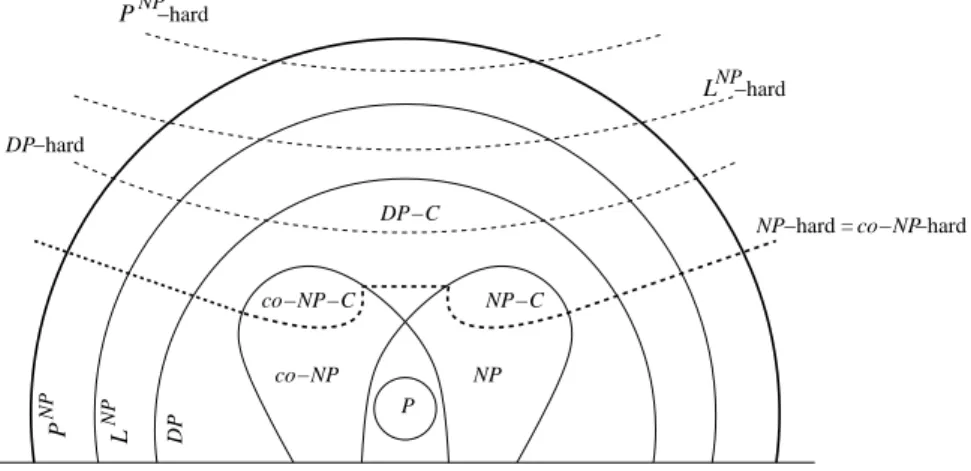
2), which contain the decision problems which can be solved by applying, with a number of calls which is polynomial (respectively, logarithmic) with respect to the size of the instance, a subprogram able to solve an appropriate problem in NP (usually, an NP-complete problem); and the class DP [15] (or DIFP [2] or BH2[11], [17], . . .) as the class of languages (or problems) L such that there are two languages L1 ∈ NP and L2∈ co-NP satisfying L = L1∩ L2. This class is not to be confused with NP ∩ co-NP (see the warning in, e.g., [14,
NP −hard L −hard DP NP −hard P L NP P NP co−NP NP NP−C P DP−C
NP−hard = co−NP−hard
co−NP−C
DP
Figure 1: Some classes of complexity.
p. 412]); actually, DP contains NP ∪ co-NP and is contained in LN P. See Figure 1.
Membership to P, NP, co-NP, DP, LN P or PN P gives an upper bound on the complexity of a problem (this problem is not more difficult than . . .), whereas a hardness result gives a lower bound (this problem is at least as difficult as . . .). Still, such results are conditional in the sense that we do not know whether or where the classes of complexity collapse.
We now consider some of the problems from Section 1.1.
Proposition 2 [12], [6, pp. 56–60 and pp. 199-200] The decision prob-lems HAMC and HAMP, in an undirected, directed or oriented graph, are
NP-complete. ♦
The problems VC, SAT and 3-SAT are also three of the basic and most well-known NP-complete problems [4], [6, p. 39, p. 46, p. 190 and p. 259]. More generally, k-SAT is NP-complete for k ≥ 3 and polynomial for k = 2. The problem 1-3-SAT, which is obvioulsy in NP, is also NP-complete [16, Lemma 3.5], [6, p. 259], [9, Rem. 3].
The following results will be used in the sequel.
Proposition 3 [9] For every integer k ≥ 3, the decision problems U-SAT, U-k-SAT and U-1-3-SAT have equivalent complexity, up to polynomials. ♦ Using the previous proposition and results from [2] and [14, p. 415], it is rather simple to obtain the following two results.
Proposition 4 For every integer k ≥ 3, the decision problems U-SAT, U-k-SAT and U-1-3-SAT are NP-hard (and co-NP-hard by Remark 1). ♦
Proposition 5 For every integer k ≥ 3, the decision problems U-SAT,
U-k-SAT and U-1-3-SAT belong to the class DP. ♦
Remark 6 It is not known whether these problems are DP-complete. In [14, p. 415], it is said that “U-SAT is not believed to be DP-complete”. Proposition 7 [8] The decision problems U-SAT and U-VC have equiva-lent complexity, up to polynomials. In particular, there exists a polynomial
reduction from U-1-3-SAT to U-VC: U-1-3-SAT →p U-VC. ♦
After the following remark is made, we shall be ready to investigate the problems of uniqueness of Hamiltonian cycle or path.
Remark 8 In [13], it is shown that the following problem is PN P-complete (or ∆2-complete).
ProblemU-OTS (Unique Optimal Travelling Salesman):
Instance: A set of n vertices, a n × n symmetric matrix [cij] of (nonneg-ative) integers giving the distance between any two vertices i and j. Question: Is there a unique optimal tour, that is, a unique way of visiting every vertex exactly once and coming back, with the smallest distance sum? At best, a polynomial reduction from any instance G = (V, E) of U-HAMC[U] to U-OTS would show that U-HAMC[U] belongs to PN P, but we have a bet-ter result in Theorem 15(b), with U-HAMC[U] belonging to DP; no useful information for our Hamiltonian problems can be induced from this result on U-OTS.
2
Locating the Problems of Uniqueness
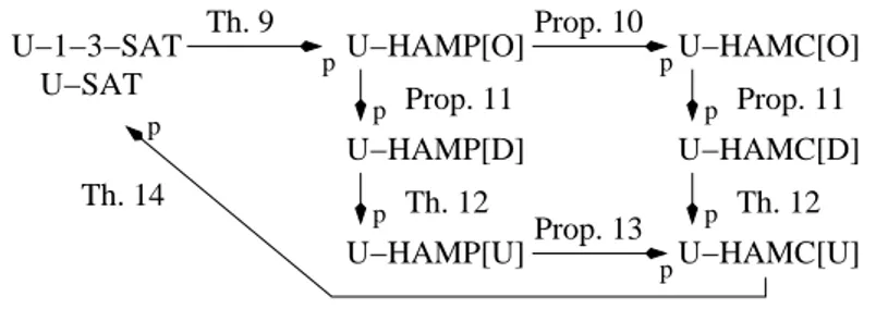
We prove that our six Hamiltonian problems have the same complexity as any of the three problems U-SAT, U-k-SAT (k ≥ 3) and U-1-3-SAT by proving the chain of polynomial reductions given by Figure 2.
Theorem 9 There exists a polynomial reduction from 1-3-SAT to
U-HAMP[O]: U-1-3-SAT →p U-HAMP[O].
Proof. We describe a polynomial reduction from the problem U-1-3-SAT to U-HAMP[O], via U-VC; it is an elaborate variation on the polynomial reduction from 3-SAT to VC in [12], [6, pp. 54–56] and the polynomial reduction from VC to HAMC[U] (see [6, pp. 56–60]). The complete proof
can be found in the Appendix. ♦
Proposition 10 There exists a polynomial reduction from U-HAMP[O] to
Th. 9 p U−HAMP[U] U−HAMC[D] U−HAMP[D] p Th. 12 p Prop. 11 Prop. 11 Th. 12 p p p p pU−HAMC[O] U−HAMC[U] Th. 14 U−SAT U−HAMP[O] U−1−3−SAT Prop. 13 Prop. 10
Figure 2: The chain of polynomial reductions.
Proof. We start from an oriented graph H = (X, A) which is an instance of U-HAMP[O] and build a graph which is an instance of U-HAMC[O] by adding two extra vertices y, z, together with the arc (y, z) and all the arcs (x, y) and (z, x), x ∈ X. This transformation is polynomial and clearly preserves the number of solutions, in particular the uniqueness. ♦ Proposition 11 There is a polynomial reduction from HAMP[O] to U-HAMP[D] and from U-HAMC[O] to U-HAMC[D]:
U-HAMP[O] →p U-HAMP[D] and U-HAMC[O] →p U-HAMC[D].
Proof. It suffices to consider the identity as the polynomial reduction. ♦ Theorem 12 There is a polynomial reduction from HAMP[D] to U-HAMP[U] and from U-HAMC[D] to U-HAMC[U]:
U-HAMP[D] →p U-HAMP[U] and U-HAMC[D] →p U-HAMC[U].
Proof. The method is borrowed from [12].
Consider any instance of U-HAMP[D] or U-HAMC[D], i.e., a directed graph H = (X, A) on n vertices. We build the undirected graph G = (V, E), the instance of U-HAMP[U] or U-HAMC[U], as follows: every vertex x ∈ X is triplicated into three vertices x− ∈ V (a minus-type vertex), x∗ ∈ V (a star-type vertex) and x+∈ V , linked by the edges x−x∗∈ E and x∗x+∈ E; for every arc (x, y) ∈ A, we create the edge x+y− in E. The graph G thus constructed has order 3n.
We claim that there is a unique Hamiltonian cycle (respectively, path) in G if and only if there is a unique directed Hamiltonian cycle (respectively, path) in H.
(1) Assume first that H admits a directed Hamiltonian cycle < x1x2. . . xn(x1) >. Then < x−1x∗1x+1x − 2x ∗ 2x+2 . . . x + n−1x − nx ∗ nx + n(x − 1) >
is a Hamiltonian cycle in G. Moreover, two different directed Hamiltonian cycles in H provide two different Hamiltonian cycles in G.
Conversely, assume that G admits a Hamiltonian cycle HC. This cycle must go through all the star-type vertices x∗, so it necessarily goes through all the edges x−x∗ and x∗x+. Without loss of generality, HC reads:
HC =< x−1x∗ 1x+1x − 2x∗2x+2 . . . x + n−1x−nx∗nx+n(x − 1) > ; (1) indeed, we may assume that we “start” with the edge x−1x∗1, then x∗1x+1; now, because the edges which have no star-type vertex as one of their extremities are necessarily of the type x+y−, the other neighbour of x+
1 is a minus-type vertex, say x−2; step by step, we see that HC has necessarily the previous form (1). Now we claim that < x1x2. . . xn−1xn(x1) > is a directed Hamiltonian cycle in H.
Indeed, for every i ∈ {1, . . . , n − 1}, the edge x+i x −
i+1 in G implies the existence of the arc (xi, xi+1) in H; the same is true for the arc (xn, x1) in H, thanks to the edge x+
nx −
1 in G. Furthermore, observe that two different Hamiltonian cycles in G provide two different directed Hamiltonian cycles in H.
So, G admits a unique Hamiltonian cycle if and only if H admits a unique directed Hamiltonian cycle.
(2) Exactly the same argument works with paths, apart from the fact that we need not consider the arc (xn, x1) in H, nor the edge x+nx−1 in G. ♦ Proposition 13 There exists a polynomial reduction from U-HAMP[U] to
U-HAMC[U]: U-HAMP[U] →p U-HAMC[U].
Proof. We start from an undirected graph G = (V, E) which is an instance of U-HAMP[U] and build a graph which is an instance of U-HAMC[U] by adding the extra vertex y, together with all the edges xy, x ∈ V . This transformation is polynomial and clearly preserves the number of solutions,
in particular the uniqueness. ♦
Theorem 14 There exists a polynomial reduction from U-HAMC[U] to
U-SAT: U-HAMC[U] →p U-SAT.
Proof. We start from an instance of U-HAMC[U], an undirected graph G = (V, E) with V = {x1, . . . , x|V |}; we assume that |V | ≥ 3. We create the set of variables X = {xi
j : 1 ≤ j ≤ |V |, 1 ≤ i ≤ |V |} and the following clauses:
(a1) for 1 ≤ i ≤ |V |, clauses of size |V |: {xi1, xi2, . . . , xi|V |}; (a2) for 1 ≤ i ≤ |V |, 1 ≤ j < j′≤ |V |, clauses of size two: {xij, x
i j′};
(b1) for 1 ≤ j ≤ |V |, clauses of size |V |: {x1j, x2j, . . . , x |V | j }; (b2) for 1 ≤ i < i′≤ |V |, 1 ≤ j ≤ |V |, clauses of size two: {xij, x
i′
(c) for 1 ≤ i < i′ ≤ |V | such that xixi′ ∈ E, for 1 ≤ j ≤ |V |, clauses/ of size two: {xi j, x i′ j+1} and {xij, x i′
j−1}, with computations performed mod-ulo |V |;
(d1) {x11};
(d2) for 2 ≤ j < j′ ≤ |V |, clauses of size two: {x2j′, x3j}.
Assume that we have a unique Hamiltonian cycle in G, HC1=< xp1xp2xp3 . . . xp|V |−1xp|V |(xp1) >. Note that for the time being, we could also write
HC1 =< xp1xp|V |xp|V |−1. . . xp3xp2(xp1) >, or “start” on a vertex other than xp1, cf. Introduction. This is why, without loss of generality, we set
p1= 1, i.e., we “fix” the first vertex, and we also choose the “direction” of the cycle, by deciding, e.g., that x2 appears “before” x3 in the cycle —cf. (d1)-(d2). Define the assignment A1 by A1(x
pq
q ) = T for 1 ≤ q ≤ |V |, and all the other variables are set FALSE by A1. We claim that A1 satisfies all the clauses.
(a1) for 1 ≤ i ≤ |V |, if the vertex xi has position j in the cycle, then the variable xi
jsatisfies the clause; (a2) if {xij, x i
j′} is not satisfied by A1for some i, j, j′, then A
1(xij) = A1(xij′) = T, which means that the vertex xi
appears at least twice in the cycle;
(b1) for 1 ≤ j ≤ |V |, if the position j is occupied by the vertex xi, then the variable xi
j satisfies the clause; (b2) if {xij, xi
′
j} is not satisfied by A1 for some i, i′, j, then two different vertices are the j-th vertex in the cycle. (c) If one of the two clauses is not satisfied, say the first one, then the positions j and j + 1 in the cycle are occupied by two vertices not linked by any edge in G.
(d1) {x11} is satisfied by A1thanks to the assumption on the first vertex of the cycle; (d2) if for some j < j′, the clause {x2j′, x3j} is not satisfied,
then the vertex x3 occupies a position j smaller than the position j′ of x2, which contradicts our assumption on x2 and x3.
Is A1 unique? Assume on the contrary that another assignment, A2, also satisfies the constructed instance of U-SAT. Then by (a1) and (a2), for every i ∈ {1, . . . , |V |}, there is at least, then at most, one j = j(i) such that A2(xij) = T; by (b1) and (b2), for every j ∈ {1, . . . , |V |}, there is at least, then at most, one i = i(j) such that A2(xij) = T; so we have “a place for everything and everything in its place”, with exactly |V | variables which are TRUE by A2 and an ordering of the vertices according to the one-to-one correspondence given by A2: the vertex xiis in position j if and only if A2(xij) = T. Next, thanks to the clauses (c), two vertices following each other in this ordering, including the last and first ones, are necessarily neighbours, so that this ordering is a Hamiltonian cycle, HC2. Since we have assumed the uniqueness of the Hamiltonain cycle HC1 in G, the two cycles can differ only by their starting points or their “directions”. However these differences are ruled out by the clauses (d1) and (d2), so that the two
cycles coincide vertex to vertex, and A1 = A2. So a YES answer for U-HAMC[U] leads to a YES answer for U-SAT.
Assume now that the answer to U-HAMC[U] is negative. If it is negative because there are at least two Hamiltonian cycles, then we have at least two assignments satisfying the instance of U-SAT: we have seen above how to construct a suitable assignment from a cycle, and different cycles obviously lead to different assignments. If there is no Hamiltonian cycle, then there is no assignment satisfying U-SAT, because such an assignment would give a cycle, as we have seen above with A2. So in both cases, a NO answer to
U-HAMC[U] implies a NO answer to U-SAT. ♦
Gathering all our previous results, we obtain the following theorem. Theorem 15 For every integer k ≥ 3, the decision problems U-SAT, k-SAT and 1-3-SAT have the same complexity as HAMP[U], U-HAMC[U], U-HAMP[O], U-HAMC[O], U-HAMP[D], and U-HAMC[D], up to polynomials. Therefore,
(a) the decision problems HAMP[U], HAMC[U], HAMP[O], U-HAMC[O], U-HAMP[D], and U-HAMC[D] are NP-hard (and co-NP-hard by Remark 1);
(b) the decision problems HAMP[U], HAMC[U], HAMP[O],
U-HAMC[O], U-HAMP[D], and U-HAMC[D] belong to the class DP. ♦
Note that the membership to DP could have been proved directly.
3
Conclusion
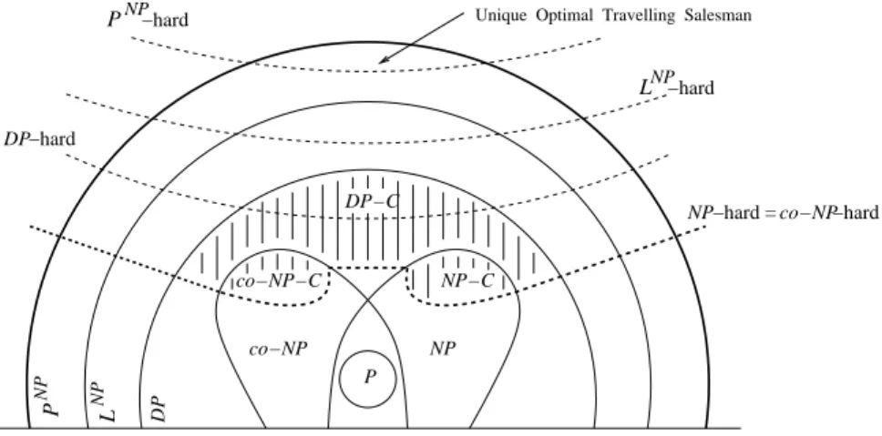
By Theorem 15, for every integer k ≥ 3, the three decision problems U-SAT, U-k-SAT, U-1-3-SAT have the same complexity, up to polynomials, as the problem of the uniqueness of a path or of a cycle in a graph, undirected, directed, or oriented; all are NP-hard (and co-NP-hard by Remark 1) and belong to the class DP, and it is thought that they are not DP-complete. Anyway, they can be found somewhere in the hatched area of Figure 3. Open problem. Find a better location for any of these problems inside the hierarchy of complexity classes.
In [2], the authors wonder whether
(A) U-SAT is NP-hard, but here we believe that what they mean is: does there exist a polynomial reduction from an NP-complete problem to U-SAT ? i.e., they use the second definition of NP-hardness;
finally, they show that (A) is true if and only if (B) U-SAT is DP-complete.
So, if one is careless and considers that U-SAT is NP-hard without checking according to which definition, one might easily jump too hastily to the
NP −hard L −hard DP L NP P NP co−NP NP NP−C P DP−C
NP−hard = co−NP−hard
co−NP−C
DP
Unique Optimal Travelling Salesman
NP
P −hard
Figure 3: Some classes of complexity: Figure 1 re-visited.
conclusion that U-SAT is DP-complete, which, to our knowledge, is not known to be true or not. As for U-3-SAT, we do not know where to locate it more precisely either; in [3] the problems U-k-SAT and more particularly U-3-SAT are studied, but it appears that they are versions where the given set of clauses has zero or one solution, which makes quite a difference with our problem.
Appendix: the Proof of Theorem 9
A) From U-1-3-SAT to U-VC
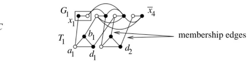
From an arbitrary instance of U-1-3-SAT with m clauses and n variables, we mimick the reduction from 3-SAT to VC in [12], [6, pp. 54–56], and we construct the instance GV C= (VV C, EV C) of U-VC as follows (see Figure 4 for an example): we construct for each clause cja triangle Tj= {aj, bj, dj}, and for each variable xi a component Gi= (Vi= {xi, xi}, Ei= {xixi}). Then we link the components Gi on the one hand, and the triangles Tj on the other hand, according to which literals appear in which clauses (“membership edges”). For each clause cj = {ℓ1, ℓ2, ℓ3}, we also add the triangular set of edges E′
j= {ℓ1ℓ2, ℓ1ℓ3, ℓ2ℓ3}. Finally, we set k = n + 2m.
The order of GV Cis 3m + 2n and its number of edges is at most n + 9m (the edge sets E′
jare not necessarily disjoint).
Note already that if V∗is a vertex cover, then each triangle Tjcontains at least two vertices, each component Gi at least one vertex, and |V∗| ≥ 2m + n = k; if |V∗| = 2m + n, then each triangle contains exactly two vertices, and each component Giexactly one vertex. We can also observe that, because of the edge sets Ej, at least two vertices among ℓ1′ , ℓ2, ℓ3 belong to any vertex cover.
x4 a1 d2 1 b 1 d 1 G x1 membership edges 1 T
G
VCFigure 4: Illustration of the undirected graph constructed for the re-duction from U-1-3-SAT to U-VC, with four variables and two clauses, c1 = {x1, x2, x3}, c2 = {x2, x3, x4}. Here, k = 8, and the black vertices form the (not unique) vertex cover V∗ of size eight corresponding to the (not unique) truth assignment x1= T, x2= F, x3= F, x4= F 1-3-satisfying the clauses. As soon as we set V∗∩ (V
1∪ V2∪ V3∪ V4) = {x1, x2, x3, x4}, the other vertices in V∗are forced.
truth assignment 1-3-satisfying the clauses of C. Then, by taking, in each Gi, the vertex corresponding to the literal which is TRUE, and in every triangle Tj, the two vertices which are linked to the two false literals of cj, we obtain a vertex cover V∗ whose size is equal to k. Moreover, once we have put the n vertices corresponding to the true literals in the vertex cover V∗in construction, we have
no choice for the completion of V∗with k − n = 2m vertices: when we take two vertices in Tj, we must take the two vertices which cover the membership edges linked to the two false literals (in the example of Figure 4, the vertices b1, d1 and b2, d2). So, if another vertex cover V+ of size k exists, it must have a different distribution of its vertices over the components Gi, still with exactly one vertex in each Gi; this in turn defines a valid truth assignment, by setting xi = T if xi ∈ V+
, xi = F if xi ∈ V+
. Now this assignment 1-3-satisfies C, thanks in particular to our observation on the covering of the edges in Ej. So we have two′ truth assignments 1-3-satisfying C, contradicting the YES answer to U-1-3-SAT; therefore, V∗is the only vertex cover of size k.
(b) Assume next that the answer to U-1-3-SAT is NO: this may be either because no truth assignment 1-3-satisfies the instance, or because at least two assignments do; in the latter case, this would lead, using the same argument as in the previous paragraph, to at least two vertex covers of size k, and a NO answer to U-VC. So we are left with the case when the set of clauses C cannot be 1-3-satisfied. But again, we have already seen that this would imply that no vertex cover of size (at most) k exists, since such a hypothetical vertex cover V+ would imply the existence of a suitable assignment.
We are now ready to construct an instance of U-HAMP[O]. In the sequel, we shall say “path” for “directed Hamiltonian path”.
B) Construction of the Instance of U-HAMP[O]
We look deeper into the proof of the NP-completeness of the problem Hamilto-nian Cycle (see [6, pp. 56–60]), which uses a polynomial reduction from VC to HAMC[U] that, due to the so-called “selector vertices”, cannot cope with the
(u,e,5) (v,e,1) (v,e,2) (v,e,4) (v,e,5) (u,e,2) (u,e,3) (u,e,6) (u,e,4) (v,e,6) (v,e,3)
u
6
1
(u,e,1)v
Figure 5: Two possible representations of the same component Hefor the edge e = uv ∈ EV C (Step 1).
problem of uniqueness; step by step, we construct an oriented graph H = (X, A) for which we will prove that:
(i) if there is a YES answer for the instance of U-1-3-SAT (which implies that there is a unique vertex cover V∗in GV C, with cardinality at most k), then there is a unique path in H;
(ii) if there are at least two assignments 1-3-satisfying all the clauses (i.e., there are at least two vertex covers in GV C, with cardinality at most k), then there are at least two paths in H;
(iii) if there is no assignment 1-3-satisfying the clauses (and no vertex cover in GV C with cardinality at most k), then there is no path in H.
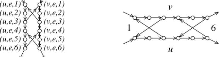
Step 1. For each edge e = uv ∈ EV C, we build one component He = (Xe, Ae) with 12 vertices and 14 arcs: Xe = {(u, e, i), (v, e, i) : 1 ≤ i ≤ 6}, Ae = {((u, e, i), (u, e, i + 1)), ((v, e, i), (v, e, i + 1)) : 1 ≤ i ≤ 5} ∪ {((v, e, 3), (u, e, 1)), ((u, e, 3), (v, e, 1))} ∪ {((v, e, 6), (u, e, 4)), ((u, e, 6), (v, e, 4))}; see Figure 5, which is the oriented copy of Figure 3.4 in [6, p. 57].
In the completed construction, the only vertices from this component that will be involved in any additional arcs are the vertices (u, e, 1), (u, e, 6), (v, e, 1), and (v, e, 6). This, together with the fact that there will be two particular vertices, α1 and δ, which will necessarily be the ends of any path, will imply that any path in the final graph H will have to meet the vertices in Xein exactly one of the three configurations shown in Figure 6, which is the oriented copy of Figure 3.5, in [6, p. 58]. Thus, when the path meets the component He at (u, e, 1), it will have to leave at (u, e, 6) and go through either (a) all 12 vertices in the component, in which case we shall say that the component is completely visited from the u-side, or (b) only the 6 vertices (u, e, i), 1 ≤ i ≤ 6, in which case we shall say that the component is visited in parallel and needs two visits, i.e., another section of the path will re-visit the component, meeting the 6 vertices (v, e, i), 1 ≤ i ≤ 6. Step 2. We create n vertices αi, 1 ≤ i ≤ n, and 2n arcs (αi, (xi, xixi, 1)), (αi, (xi, xixi, 1)), that is, we link αito the “first” vertices of the component He whenever e = xixi. The vertices αi can be seen as literal selectors that will choose between xi and xi. The vertex α1 will have no other neighbours; this means in particular that it will have no in-neighbours, thus it will necessarily be the starting vertex of any Hamiltonian path, if such a path exists.
(u,e,6) (u,e,6) (v,e,6)
(v,e,1)
(v,e,6)
(a)
(b)
(c)
(u,e,1) (u,e,1) (v,e,1)
Figure 6: The three ways of going through the component He (Step 1). The arrows inside Heare not represented.
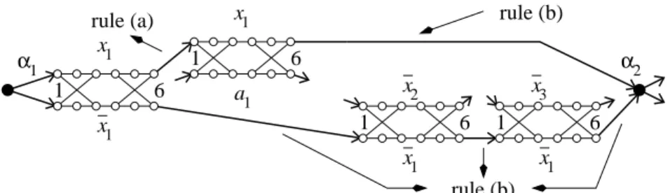
x1 x1 x1 a1 x1 x1 x2 x3 α2 6 1 rule (a) 1 6 rule (b) rule (b) 1 1 6 6 1 α
Figure 7: The example of the literals x1 and x1 from Figure 4 (Step 2); here, Rule (a) applies with q(x1) = 1, q(x1) = 0, Rule (b) with s(x1) = 2. The arrows inside Heare not represented.
We choose an arbitrary order on the 3m vertices of the triangles Tj in the graph GV C, say OT =< a1, b1, d1, a2, . . . , dm > and an arbitrary order on the literals xi, xi, say Oℓ =< x1, x2, . . . , xn, x1, . . . , xn >. For each literal ℓi equal to xior xi, we do the following (see Figure 7 for an example):
Rule (a): If ℓi appears q = q(ℓi) ≥ 0 times in the clauses and is linked in GV C to t1, . . . , tq where the t’s belong to the triangles Tj and follow the or-der OT, then we create the arcs ((ℓi, ℓiℓi, 6), (ℓi, ℓit1, 1)), ((ℓi, ℓit1, 6), (ℓi, ℓit2, 1)), . . ., ((ℓi, ℓitq−1, 6), (ℓi, ℓitq, 1)).
Rule (b): We consider the triangular sets of edges E′
j described in the con-struction of GV C.
• If ℓi does not belong to any such edge, we create the arc ((ℓi, ℓitq, 6), αi+1) —or ((ℓi, ℓiℓi, 6), αi+1) if ℓi does not apppear in any clause— unless i = n, in which case we create ((ℓi, ℓitq, 6), β1) or ((ℓi, ℓiℓi, 6), β1), where β1is a new vertex that will be spoken of at the beginning of Step 3.
• If ℓi belongs to s = s(ℓi) > 0 edges from E′j, which link ℓi to s literals ℓi1, . . . , ℓisthat follow the order Oℓ, then we build the arc ((ℓi, ℓitq, 6), (ℓi, ℓiℓi1, 1))
—or the arc ((ℓi, ℓiℓi, 6), (ℓi, ℓiℓi1, 1)) if q = 0; next, the arcs ((ℓi, ℓiℓi1, 6), (ℓi,
d1 β1
’
x2 β1 6 1 1 b1 b1 6 1 b1 a a1 6 1 1 a x1 1 1 d x3 rule (a) rule (b) (b) (c) (c) (c) (c) (b) (b) (b) d1 1 1 2 β rule (a) 6 63 components corresponding to membership edges
6
Figure 8: The treatment of the triangle T1 from Figure 4 (Step 3). The arrows inside Heare not represented.
in which case we create ((ℓi, ℓiℓis, 6), β1).
Remark 16 In the example of Figure 7, one can see that if a path takes, e.g.,
the arc (α1, (x1, x1x1, 1)), then it visits the vertices (x1, x1x1, 6), (x1, x1a1, 1), (x1, x1a1, 6), and α2. If on the other hand, we use the arc (α1, (x1, x1x1, 1)), we
also go to α2. The same is true between α2 and α3, . . ., between αn−1 and αn,
between αnand β1.
We can see that so far, α1 has (out-)degree 2, α2, . . ., αnhave degree 4 (in- and out-degrees equal to 2), and β1 has (in-)degree 2.
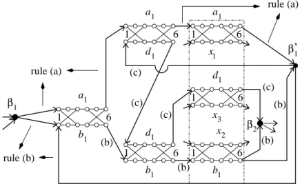
Step 3. We consider the m clauses and the m corresponding triangles Tj. We create 2m vertices βj, β′j, 1 ≤ j ≤ m. As we have seen in the previous step, β1has already two in-neighbours, which can be (ℓn, ℓntq, 6), or (ℓn, ℓnℓn, 6), or (ℓn, ℓnℓns, 6). We also create one more vertex δ, which will have only
in-neighbours, so that α1 and δ will necessarily be the ends of any directed Hamil-tonian path, if such a path exists.
Now for the triangle Tj= {aj, bj, dj}, 1 ≤ j ≤ m, associated to the clause cj= {ℓj1, ℓj2, ℓj3} in the graph GV C, we consider the six corresponding components
Hajbj, Hajdj, Hbjdj, Hajℓj1, Hbjℓj2 and Hdjℓj3. The vertices βj and β
′ j can be seen as triangle selectors, intended to choose two vertices among three. With this in mind, we create the following arcs (see Figure 8), for j ∈ {1, 2, . . . , m}:
Rule (a): (βj, (aj, ajbj, 1)), ((aj, ajbj, 6), (aj, ajdj, 1)), ((aj, ajdj, 6), (aj, ajℓj1,
1)), ((aj, ajℓj1, 6), β
′
Rule (b): (βj, (bj, ajbj, 1)), (β′j, (bj, ajbj, 1)), ((bj, ajbj, 6), (bj, bjdj, 1)), ((bj, bjdj, 6), (bj, bjℓj2, 1)), ((bj, bjℓj2, 6), β′j), plus the arc ((bj, bjℓj2, 6), βj+1), unless
j = m, in which case it is ((bj, bjℓj2, 6), δ).
Rule (c): (βj, (dj, ajdj, 1)), ((dj, ajdj, 6), (dj, bjdj, 1)), ((dj, bjdj, 6), (dj, djℓj′
3,
1)), ((dj, djℓj3, 6), βj+1), unless j = m, in which case it is ((dj, djℓj3, 6), δ).
Remark 17 In the example of Figure 8, there are three ways for going from β1
to β2 through the components Ha1b1, Ha1d1 and Hd1b1.
• If a path starts by taking the arc (β1, (a1, a1b1, 1)), then there are two
possibil-ities, according to how we visit Ha1b1:
◦ The first possibility corresponds to taking a1 and d1, not b1, in a vertex
cover: the path completely visits the component Ha1b1 from the a1-side, then the
component Ha1d1 in parallel, then the component Ha1x1 in a so far unspecified
way, then β′
1.
Next, it takes the arc (β′1, (d1, d1a1, 1)), re-visits Hd
1a1 in parallel, completely
visits Hd1b1 from the d1-side, then Hd1x3, and ends this path section at β2. One
can see that the three components corresponding to edges incident to b1 must all
be completely visited from the side opposite b1, including the x2-side.
◦ The second possibility corresponds to taking a1 and b1, not d1, in a vertex
cover: the path follows the arc (β1, (a1, a1b1, 1)), visits Ha1b1 in parallel, visits
completely Ha1d1 from the a1-side, then Ha1x1, and β
′
1.
Next, it takes the arc (β1, (b1, b1a1′ , 1)), goes through Hb
1a1 in parallel, goes
completely through Hb1d1 from the b1-side, then Hb1x2, and ends this path section
at β2. The component Hd1x3 is not yet visited.
• Alternatively, a path can start by taking the arc (β1, (b1, a1b1, 1)); this
corre-sponds to taking b1 and d1, not a1, in a vertex cover and constitutes the third way
for going from β1 to β2. The path then completely visits Hb1a1 from the b1-side,
Hb1d1 in parallel, Hb1x2, and β
′
1.
Next, it completely visits Hd1a1 from the d1-side, Hd1b1 in parallel, Hd1x3,
and this path section ends at β2. The component Ha1x1 is not yet visited.
It is easy to see that these are the only three ways for going from β1to β2through
the components Ha1b1, Ha1d1 and Hd1b1, not taking into account the ways of
going through the components Ha1x1, Hb1x2 and Hd1x3 (this issue will be treated
later on, in the general case): indeed, the only possibility left would be to follow the arc (β1, (b1, a1b1, 1)) and visit Hb1a1 in parallel, but then the a1-side of Hb1a1
cannot be reached.
The same will be true for the components Hajbj, Hajdj and Hdjbj and the
corre-sponding triangles Tj, 1 ≤ j ≤ m, between βjand βj+1 (or between βm and δ). The description of the oriented graph H is complete. Now β1 has increased its degree to 4, and β2, . . ., βm and β′
1, . . ., βm′ have degree 4. Actually, all the
selectors but α1 have in-degree 2 and out-degree 2 in H. These n selectors αi, 1 ≤ i ≤ n, and 2m selectors βj, βj, 1 ≤ j ≤ m, translate the choices we have′ to make when constructing a vertex cover with size 2m + n: we have one choice among the n variables (take xior xi); as for the m triangles Tjassociated to the
clauses, Remark 17 has shown how the selectors βj, βj, 1 ≤ j ≤ m, can be used′ to choose two vertices among three. The number of selectors is one reason why there is no directed Hamiltonian path in H when the vertex covers in GV C have size at least 2m + n + 1.
The order of H is 12|EV C|+n+2m+1, which is at most 12(n+9m)+n+2m+1, so that the transformation is polynomial indeed.
We are now going to prove our claims about the existence or non-existence, uniqueness or non-uniqueness, of a directed Hamiltonian path in H.
C) How it Works
Assume first that there is an assignment satisfying the instance of U-1-3-SAT, and therefore that there is a vertex cover V∗in GV Cwith size 2m + n. We construct a path in H in a straightforward way: every component Huv (uv ∈ EV C) with {u, v} ⊂ V∗ is visited in parallel, whereas Huv is completely visited from the u-side whenever u ∈ V∗, v /∈ V∗. Let us have a closer look at how this works:
We start at α1, and visit completely the component Hx1x1 from the x1-side
if x1 = T, from the x1-side if x1 = F (or, equivalently, if x1 ∈ V∗ or x1 ∈ V∗, respectively). If, say, x1= F, we then completely go through all the components corresponding to triangles Tj and involving x1, all from the x1-side; note that all the components just completely visited involve x1 and a vertex not in V∗, by the very construction of the vertex cover V∗, which is possible because it stems from an assignment 1-3-satisfying all the clauses. Then we go through the components constructed from the edge sets E′
jand involving x1; those involving a second vertex in V∗ (i.e., a true literal) are visited in parallel, whereas those involving a vertex not in V∗ are completely visited from the x1-side; then the path arrives at α2. The components involving x1, apart from Hx1x1, remain
completely unvisited for the time being, and the components that have been visited in parallel will have to be re-visited.
We act similarly between α2and α3, . . ., αnand β1; cf. Remark 16. When do-ing this, we re-visit all the components that had been visited only in parallel, and completely visit the components involving a literal not in V∗and corresponding to edges in Ej. The only components not visited yet between α1′ and β1are those corresponding to edges between a false literal (not in V∗) and its neighbours in the triangles Tj.
Next, starting from β1, we use Remark 17 according to the three possible cases: (a) {a1, d1} ⊂ V∗, b1∈ V/ ∗, (b) {a1, b1} ⊂ V∗, d1∈ V/ ∗, (c) {b1, d1} ⊂ V∗, a1 ∈ V/ ∗. We give in detail only the third case, for the clause c1 = {ℓ1, ℓ2, ℓ3}: we use the arc (β1, (b1, a1b1, 1)) and completely visit the component Ha1b1 from
the b1-side, then the component Hb1d1 in parallel, then the complete component
Hb1ℓ2 from the b1-side (because if b1 ∈ V
∗, then ℓ2 ∈ V/ ∗ and this component had not yet been visited) and end at β1. Next, we take the arc (β′ 1, (d1, d1a1, 1)),′ we completely visit Hd1a1 from the d1-side, re-visit Hd1b1 in parallel, completely
visit Hd1ℓ3 from the d1-side, and this path section ends at β2. Note that (a) the
three components involving a1 between β1and β2 have been completely visited, from the b1-, d1- or ℓ1-sides (because a1 ∈ V/ ∗ implies that ℓ1∈ V∗); (b) any so far unvisited component involving a false literal (here, these are ℓ2 and ℓ3) and
one of the vertices of the triangle T1 (here b1 and d1) has now been completely visited from the triangle sides (here from the b1- and d1-sides).
We act similarly between β2and β3, . . ., βmand δ; cf. the end of Remark 17. The ultimate section takes us between βm and δ, the final vertex, and we have indeed built a directed Hamiltonian path, from α1to δ, in the oriented graph H. Obviously, two different assignments 1-3-satisfying all the clauses lead, following the above process, to two different paths in H. We still want to prove that 1) if no assignment 1-3-satisfying all the clauses exists, then no path exists, and 2) a unique assignment 1-3-satisfying all the clauses leads to a unique path.
1) We assume that there is a directed Hamiltonian path HP in H, and exhibit an assignment 1-3-satisfying all the clauses.
Let us consider the vertex α1; its two out-neighbours in H are (x1, x1x1, 1) and (x1, x1x1, 1). So exactly one of the arcs (α1, (x1, x1x1, 1)), (α1, (x1, x1x1, 1)) is part of HP. The same is true for αi, 1 < i ≤ n. As a consequence, we can define a valid assignment of the variables xi, 1 ≤ i ≤ n, by setting xi= T if and only if the arc (αi, (xi, xixi, 1)) belongs to HP.
Next, we address the vertices βj, 1 ≤ j ≤ m. The construction in Steps 2 and 3 is such that each vertex βj, 1 ≤ j ≤ m, has two out-neighbours, (aj, ajbj, 1) and (bj, ajbj, 1).
This implies that the assignment defined above is such that there is at least one true literal in each clause. Indeed, if we assume that the clause cj = {ℓj1, ℓj2, ℓj3} does not contain any true literal, then the component Hajℓj1 is
completely visited by HP from the aj-side, because ℓj1 = F implies that the arc
(αj, (ℓj1, ℓj1ℓj1, 1)) is not part of HP and does not give access to the ℓj1-side.
Similarly, the components Hbjℓj2 and Hdjℓj3 are completely visited by HP from
the bj- and dj-sides, respectively. This in turn implies that in HP we have the arcs ((aj, ajℓj1, 6), β
′
j), (βj, (aj, ajbj, 1)), ((dj, djℓj3, 6), βj+1) and (β
′
j, (dj, djaj, 1)) — replace βj+1 by δ if j = m. Now how does HP go through (bj, bjℓj2, 6)? It
cannot be with the help of the ℓj2-side of Hbjℓj2, so there are only two
possibili-ties left: but if it is with the arc ((bj, bjℓj2, 6), β
′
j), then βj′ has three neighbours in HP, which is impossible; and if it is with the arc ((bj, bjℓj2, 6), βj+1), then
in HP, the vertex βj+1 has two in-neighbours, which is impossible —including when j = m and βj+1is replaced by δ. From this we can conclude that the clause cj= {ℓj1, ℓj2, ℓj3} contains at least one true literal.
Assume next that one clause has at least two true literals: without loss of generality, cj= {ℓj1, ℓj2, ℓj3} is such that ℓj1= ℓj2 = T. Then HP has no access
to the ℓj1- and ℓj2- sides of the components involving ℓj1or ℓj2, but, since there is
the edge ℓj1ℓj2in GV C, this means that HP has no way of visiting the component
Hℓ
j1ℓj2. Therefore, we have just established that the assignment derived from
the path HP 1-3-satisfies all the clauses. This, together with the fact that two assignments 1-3-satisfying the clauses lead to two paths, shows that a NO answer to the instance of U-1-3-SAT implies a NO answer for the constructed instance H of U-HAMP[O].
2) We want to show that a unique assignment A 1-3-satisfying all the clauses leads to a unique path in H. This assignment leads to a unique vertex cover V∗, of size n + 2m, in GV C, and to a path in H, as already seen. Now assume that
we have a second path, so that these two paths, which we call HP1 and HP2, both lead, with the above description in 1), to the same A and the same V∗.
The two paths must behave in the same way over the components Hxixi,
1 ≤ i ≤ n: otherwise, from them we could define two different valid assignments, which would both, as seen previously, 1-3-satisfy the clauses.
Next, consider the clause cj= {ℓj1, ℓj2, ℓj3} and assume without loss of
gener-ality that A(ℓj1) = T, A(ℓj2) = A(ℓj3) = F; this implies, for both HP1and HP2,
that the components Hℓj1ℓj1, Hℓj2ℓj2 and Hℓj3ℓj3 are completely visited from the ℓj1-, ℓj2- and ℓj3-sides, respectively, so that both paths have no access to the
ℓj2- nor ℓj3-sides. As a consequence, between βj and βj+1 (or βm and δ), the
components Hbjℓj2 and Hdjℓj3 are completely visited from the bj- and dj-sides,
respectively. Then necessarily the following arcs belong to HP1 and HP2, going along the dj-side:
((dj, djℓj3, 6), βj+1) —or ((dj, djℓj3, 6), δ)—, ((dj, djbj, 6), (dj, djℓj3, 1)), ((dj, djaj,
6), (dj, djbj, 1)), (βj, (dj, djaj, 1));′ and going along the bj-side: ((bj, bjℓj2, 6), β
′
j) (because βj+1 —or δ— cannot have two in-neighbours), and
((bj, bjdj, 6), (bj, bjℓj2, 1)), ((bj, bjaj, 6), (bj, bjdj, 1)).
The component Hbjdj must be visited in parallel, and it is (βj, (bj, bjaj, 1))
that belongs to the two paths.
We can see that all the components containing aj, in particular Hajℓj1, must
be completely visited from the sides opposite aj. So far, we have proved that the two paths HP1and HP2behave identically between βjand βj+1(or βmand δ), including on the components corresponding to membership edges (between liter-als and triangles).
Consider now what happens between αi and αi+1 (or αn and β1). Assume without loss of generality that, say, A(xi) = T, so that (αi, (xi, xixi, 1)) is part of the two paths. Consider the components involving xi in H: there are first those involving vertices of type a, b or d, which translate the membership of xi to a certain number of clauses, and which we called t1, . . . , tq in Step 2(a); we have already seen in the previous paragraph that these components must be completely visited from the xi-side.
Then we consider the components created from the edges in E′j, cf. Step 2(b); here, some edges in GV C can have both ends in V∗, but, using similar arguments as before, we can see that the two paths will visit all these components in the same way: consider the clause cj= {ℓj1, ℓj2, ℓj3} and the corresponding set E
′ j, and assume without loss of generality that xi = ℓj1, so that A(ℓj1) = T, which
implies that A(ℓj2) = A(ℓj3) = F; then Hℓj1ℓj2 and Hℓj1ℓj3 must be completely visited from the ℓj2- and ℓj3-sides, respectively, and Hℓj2ℓj3 in parallel, i.e., the two paths have no choice but to behave identically on all three components. As for the components with xi, they must be completely visited from the side which is not the side of xi.
So we have just proved that the two paths are identical between α1 and α2, . . ., αnand β1.
References
[1] J.-P. BARTH´ELEMY, G. D. COHEN and A. C. LOBSTEIN: Algo-rithmic Complexity and Communication Problems, London: Univer-sity College of London, 1996.
[2] A. BLASS and Y. GUREVICH: On the unique satisfiability problem, Information and Control, Vol. 55, pp. 80-88, 1982.
[3] C. CALABRO, R. IMPAGLIAZZO, V. KABANETS and R. PATURI: The complexity of Unique k-SAT: an isolation lemma for k-CNFs, Journal of Computer and System Sciences, Vol. 74, pp. 386–393, 2008. [4] S. A. COOK: The complexity of theorem-proving procedures, Pro-ceedings of 3rd Annual ACM Symposium on Theory of Computing, pp. 151–158, 1971.
[5] T. CORMEN: Algorithmic complexity, in: K. H. Rosen (ed.) Hand-book of Discrete and Combinatorial Mathematics, pp. 1077–1085, Boca Raton: CRC Press, 2000.
[6] M. R. GAREY and D. S. JOHNSON: Computers and Intractability, a Guide to the Theory of NP-Completeness, New York: Freeman, 1979. [7] L. HEMASPAANDRA: Complexity classes, in: K. H. Rosen (ed.) Handbook of Discrete and Combinatorial Mathematics, pp. 1085–1090, Boca Raton: CRC Press, 2000.
[8] O. HUDRY and A. LOBSTEIN: Complexity of unique (optimal) solu-tions in graphs: Vertex Cover and Domination, Journal of Combina-torial Mathematics and CombinaCombina-torial Computing, to appear.
[9] O. HUDRY and A. LOBSTEIN: Some complexity considerations on the uniqueness of solutions for satisfiability and colouring problems, submitted.
[10] O. HUDRY and A. LOBSTEIN: Unique (optimal) solutions: complex-ity results for identifying and locating-dominating codes, submitted. [11] D. S. JOHNSON: A catalog of complexity classes, in: Handbook of
Theoretical Computer Science, Vol. A: Algorithms and Complexity, van Leeuwen, Ed., Chapter 2, Elsevier, 1990.
[12] R. M. KARP: Reducibility among combinatorial problems, in: R. E. Miller and J. W. Thatcher (eds.) Complexity of Computer Computa-tions, pp. 85–103, New York: Plenum Press, 1972.
[13] C. H. PAPADIMITRIOU: On the complexity of unique solutions, Journal of the Association for Computing Machinery, Vol. 31, pp. 392-400, 1984.
[14] C. H. PAPADIMITRIOU: Computational Complexity, Reading: Addison-Wesley, 1994.
[15] C. H. PAPADIMITRIOU and M. YANNAKAKIS: The complexity of facets (and some facets of complexity), Journal of Computer and System Sciences, Vol. 28, pp. 244–259, 1984.
[16] T. J. SCHAEFER: The complexity of satisfiability problems, Proceed-ings of 10th Annual ACM Symposium on Theory of Computing, pp. 216–226, 1978.