Best Position Algorithms for Top-k Queries

(1)

HAL Id: inria-00378836

https://hal.inria.fr/inria-00378836

Submitted on 15 Feb 2010

HAL is a multi-disciplinary open access

archive for the deposit and dissemination of

sci-entific research documents, whether they are

pub-lished or not. The documents may come from

teaching and research institutions in France or

abroad, or from public or private research centers.

L’archive ouverte pluridisciplinaire HAL, est

destinée au dépôt et à la diffusion de documents

scientifiques de niveau recherche, publiés ou non,

émanant des établissements d’enseignement et de

recherche français ou étrangers, des laboratoires

publics ou privés.

Best Position Algorithms for Top-k Queries

Reza Akbarinia, Esther Pacitti, Patrick Valduriez

To cite this version:

Reza Akbarinia, Esther Pacitti, Patrick Valduriez. Best Position Algorithms for Top-k Queries.

In-ternational Conference on Very Large Data Bases (VLDB), Aug 2007, Vienna, Austria. pp.495-506.

�inria-00378836�

(2)

Best Position Algorithms for Top-k Queries

1

Reza Akbarinia

2

Esther Pacitti

Patrick Valduriez

Atlas team, LINA and INRIA University of Nantes, France

{FirstName.LastName@univ-nantes.fr, Patrick.Valduriez@inria.fr}

ABSTRACT

The general problem of answering top-k queries can be modeled using lists of data items sorted by their local scores. The most efficient algorithm proposed so far for answering top-k queries over sorted lists is the Threshold Algorithm (TA). However, TA may still incur a lot of useless accesses to the lists. In this paper, we propose two new algorithms which stop much sooner. First, we propose the best position algorithm (BPA) which executes top-k queries more efficiently than TA. For any database instance (i.e. set of sorted lists), we prove that BPA stops as early as TA, and that its execution cost is never higher than TA. We show that the position at which BPA stops can be (m-1) times lower than that of TA, where m is the number of lists. We also show that the execution cost of our algorithm can be (m-1) times lower than that of TA. Second, we propose the BPA2 algorithm which is much more efficient than BPA. We show that the number of accesses to the lists done by BPA2 can be about (m-1) times lower than that of BPA. Our performance evaluation shows that over our test databases, BPA and BPA2 achieve significant performance gains in comparison with TA.

1. INTRODUCTION

Top-k queries have attracted much interest in many different areas such as network and system monitoring [4] [8] [19], information retrieval [5] [18] [20] [26], sensor networks [27] [28], multimedia databases [10] [16] [25], spatial data analysis [11] [17], P2P systems [1] [3] [5], data stream management systems [22] [24], etc. The main reason for such interest is that they avoid overwhelming the user with large numbers of uninteresting answers which are resource-consuming.

The problem of answering top-k queries can be modeled as follows [13] [15]. Suppose we have m lists of n data items such that each data item has a local score in each list and the lists are sorted according to the local scores of their data items. And each data item has an overall score which is computed based on its local scores in all lists using a given scoring function. Then the problem is to find the k data items whose overall scores are the highest. This problem model is simple and general. Let us

illustrate with the following examples. Suppose we want to find the top-k tuples in a relational table according to some scoring function over its attributes. To answer this query, it is sufficient to have a sorted (indexed) list of the values of each attribute involved in the scoring function, and return the k tuples whose overall scores in the lists are the highest. As another example, suppose we want to find the top-k documents whose aggregate rank is the highest wrt. some given keywords. To answer this query, the solution is to have for each keyword a ranked list of documents, and return the k documents whose aggregate rank in all lists are the highest.

There has been much work on efficient top-k query processing over sorted lists. A naïve algorithm is to scan all lists from beginning to end and, maintain the local scores of each data item, compute the overall scores, and return the k highest scored data items. However, this algorithm is executed in O(m∗n) and thus it is inefficient for very large lists.

The most efficient algorithm for answering top-k queries over sorted lists is the Threshold Algorithm (TA) [14] [16] [25]. TA is applicable for queries where the scoring function is monotonic. It is simple and elegant. Based on TA, many algorithms have been proposed for top-k query processing in centralized and distributed applications, e.g. [6] [7] [9] [12] [21] [23]. The main difference between TA and previously designed algorithms, e.g. Fagin’s algorithm (FA) [13], is its stopping mechanism that enables TA to stop scanning the lists very soon. However, there are many database instances over which TA keeps scanning the lists although it has seen all top-k answers (see Example 2 in Section 3.2). And it is possible to stop much sooner.

In this paper, we propose two new algorithms for processing top-k queries over sorted lists. First, we propose the best position algorithm (BPA) which executes top-k queries much more efficiently than TA. The key idea of BPA is that its stopping mechanism takes into account special seen positions in the lists, the best positions. For any database instance (i.e. set of sorted lists), we prove that BPA stops as early as TA, and that its execution cost (called middleware cost in [15]) is never higher than TA. We prove that the position at which BPA stops can be (m-1) times lower than that of TA, where m is the number of lists. We also prove that the execution cost of our algorithm can be (m-1) times lower than that of TA. Second, based on BPA, we propose the BPA2 algorithm which is much more efficient than BPA. We show that the number of accesses to the lists done by BPA2 can be about (m-1) times lower than that of BPA. To validate our contributions, we implemented our algorithms (and TA). The performance evaluation shows that over our test databases, BPA and BPA2 outperform TA by a factor of about

1

Work partially funded by ARA “Massive Data” of the French ministry of research and the European Strep Grid4All project.

2

Partially supported by a fellowship from Shahid Bahonar University of Kerman, Iran.

Permission to copy without fee all or part of this material is granted provided that the copies are not made or distributed for direct commercial advantage, the VLDB copyright notice and the title of the publication and its date appear, and notice is given that copying is by permission of the Very Large Database Endowment. To copy otherwise, or to republish, to post on servers or to redistribute to lists, requires a fee and/or special permissions from the publisher, ACM.

VLDB ’07, September 23-28, 2007, Vienna, Austria.

(3)

(m+6)/8 and (m+1)/2 respectively, e.g. for m=10, the factor is about 2 and 5.5, respectively.

The rest of this paper is organized as follows. In Section 2, we define the problem which we address in this paper. Section 3 presents some background on FA and TA. In Sections 4 and 5, we present the BPA and BPA2 algorithms, respectively, with a cost analysis. Section 6 gives a performance evaluation of our algorithms. In Section 7, we discuss related work. Section 8 concludes.

2. PROBLEM DEFINITION

Let D be a set of n data items, and L1, L2, …, Lm be m lists such

that each list Li contains n pairs of the form (d, si(d)) where d∈D

and si(d) is a non-negative real number that denotes the local

score of d in Li. Any data item d∈D appears once and only once

in each list. Each list Li is sorted in descending order of its local

scores, hence called “sorted list”. Let j be the number of data items which are before a data item d in a list Li, then the position

of d in Li is equal to (j + 1).

The set of m sorted lists is called a database. In a distributed system, sorted lists may be maintained at different nodes. A node that maintains a list is called a list owner. In centralized systems, the owner of all lists is only one node.

The overall score of each data item d is computed as f(s1(d), s2(d),

…, sm(d)) where f is a given scoring function. In other words, the

overall score is the output of f where the input is the local scores of d in all lists. In this paper, we assume that the scoring function is monotonic. A function f is monotonic if f(x1, …, xm) ≤ f(x'1, …,

x'm) whenever xi ≤ x'i for every i. Many of the popular aggregation

functions, e.g. Min, Max, Average, are monotonic. The k data items whose overall scores are the highest among all data items, are called the top-k data items.

As defined in [15], we consider two modes of access to a sorted list. The first mode is sorted (or sequential) access by which we access the next data item in the sorted list. Sorted access begins by accessing the first data item of the list. The second mode of access is random access by which we lookup a given data item in the list. Let cs be the cost of a sorted access, and cr be the cost of a random

access. Then, if an algorithm does as sorted accesses and ar

random accesses for finding the top-k data items, then its execution cost is computed as as∗cs + ar∗cr. The execution cost

(called middleware cost in [15]) is a main metric to evaluate the performance of a top-k query processing algorithm over sorted lists [15].

Let us now state the problem we address. Let L1, L2, …, Lm be m

sorted lists, and D be the set of data items involved in the lists. Given a top-k query which involves a number k≤n and a monotonic scoring function f, our goal is to find a set D'⊆D such that D'= k, and ∀d1∈D' and∀d2∈(D-D') the overall score of d1

is at least the overall score of d2, while minimizing the execution

cost.

3. BACKGROUND

The background for this paper is the TA algorithm which is itself based on Fagin's Algorithm (FA). FA and TA are designed for processing top-k queries over sorted lists. In this section, we briefly describe and illustrate FA and TA.

3.1 FA

The basic idea of FA is to scan the lists until having at least k data items which have been seen in all lists, then there is no need to continue scanning the rest of the lists [13]. FA works as follows: 1. Do sorted access in parallel to each of the m sorted lists, and

maintain each seen data item in a set S. If there are at least k data items in S such that each of them has been seen in each of the m lists, then stop doing sorted access to the lists. 2. For each data item d involved in S, do random access as

needed to each of the lists Li to find the local score of d in Li,

compute the overall score of d, and maintain it in a set Y if its score is one of the k highest scores computed so far.

3. Return Y.

The correctness proof of FA can be found in [13]. Let us illustrate FA with the following example.

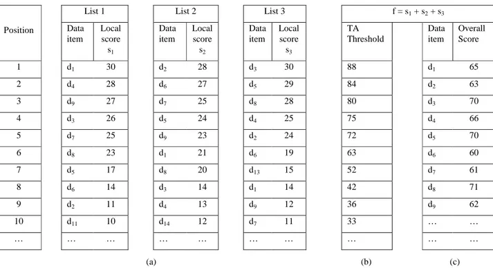
Example 1. Consider the database (i.e. three sorted lists) shown

in Figure 1.a. Assume a top-3 query Q, i.e. k=3, and suppose the scoring function computes the sum of the local scores of the data item in all lists. In this example, before position 7, there is no data item which can be seen in all lists, so FA cannot stop before this position. After doing the sorted access at position 7, FA sees d5

and d8 which are seen in all lists, but this is not sufficient for

stopping sorted access. At position 8, the number of data items which are seen in all lists is 5, i.e. d1, d3, d5, d6 and d8. Thus, at

position 8, there are at least k data items which are seen by FA in all lists, thus FA stops doing sorted access to the lists. Then, for the data items which are seen only in some of the lists, e.g. d2, FA

does random access and finds their local scores in all lists, e.g. d2

is not seen in L1 so FA needs a random access to L1 to find the

local score of d2 in this list. It computes the overall score of all

seen data items, and returns to the user the k highest scored ones.

3.2 TA

The main difference between TA and FA is their stopping mechanism which decides when to stop doing sorted access to the lists. The stopping mechanism of TA uses a threshold which is computed using the last local scores seen under sorted access in the lists. Thanks to its stopping mechanism, over any database, TA stops at a position (under sorted access) which is less than or equal to the position at which FA stops [15]. TA works as follows:

1. Do sorted access in parallel to each of the m sorted lists. As a data item d is seen under sorted access in some list, do random access to the other lists to find the local score of d in every list, and compute the overall score of d. Maintain in a set Y the k seen data items whose overall scores are the highest among all data items seen so far.

2. For each list Li, let si be the last local score seen under sorted

access in Li. Define the threshold to be δ = f(s1, s2, …, sm). If

Y involves k data items whose overall scores are higher than or equal to δ, then stop doing sorted access to the lists. Otherwise, go to 1.

(4)

3. Return Y.

The correctness proof of TA can be found in [15]. Let us illustrate TA with the following example.

Example 2. Consider the three sorted lists shown in Figure 1.a

and the query Q of Example 1, i.e. k=3 and the scoring function computes the sum of the local scores. The thresholds of the positions and the overall score of data items are shown in Figure 1.b and 1.c, respectively. TA first looks at the data items which are at position 1 in all lists, i.e. d1, d2, and d3. It looks up the local

score of these data item in other lists using random access and computes their overall scores. But, the overall score of none of them is as high as the threshold of position 1. Thus, at position 1, TA does not stop. At this position, we have Y={d1, d2, d3}, i.e. the

k highest scored data items seen so far. At positions 2 and 3, Y involves {d3, d4, d5} and {d3, d5, d8} respectively. Before position

6, none of the data items involved in Y has an overall score higher than or equal to the threshold value. At position 6, the threshold value gets 63, which is less than the overall score of the three data items involved in Y, i.e. Y={d3, d5, d8}. Thus, there are k data

items in Y whose overall scores are higher than or equal to the threshold value, so TA stops at position 6. The contents of Y at position 6 are exactly equal to its contents at position 3. In other words, at position 3, Y already contains all top-k answers. But TA cannot detect this and continues until position 6. In this example, TA does three useless sorted accesses in each list, thus a total of 9 useless sorted accesses and 9∗2 useless random accesses. In the next section, we propose an algorithm that always stops as early as TA, so it is as fast as TA. Over some databases, our algorithm can stop at a position which is (m-1) times lower than the stopping position of TA.

4. BEST POSITION ALGORITHM

In this section, we first propose our Best Position Algorithm (BPA), which is an efficient algorithm for the problem of answering top-k queries over sorted lists. Then, we analyze its execution cost and discuss its instance optimality.

4.1 Algorithm

BPA works as follows:

1. Do sorted access in parallel to each of the m sorted lists. As a data item d is seen under sorted access in some list, do random access to the other lists to find the local score and the position of d in every list. Maintain the seen positions and their corresponding local scores. Compute the overall score of d. Maintain in a set Y the k seen data items whose overall scores are the highest among all data items seen so far. 2. For each list Li, let Pi be the set of positions which are seen

under sorted or random access in Li. Let bpi, called best

position1 in Li, be the greatest position in Pi such that any

position of Li between 1 and bpi is also in Pi. Let si(bpi) be

the local score of the data item which is at position bpi in list

Li .

3. Let best positions overall score be λ = f(s1(bp1), s2(bp2), …,

sm(bpm)). If Y involves k data items whose overall scores are

higher than or equal to λ, then stop doing sorted access to the lists. Otherwise, go to 1.

4. Return Y.

1

bpi is called best because we are sure that all positions of Li

between 1 and bpi have been seen under sorted or random

access.

List 1 List 2 List 3 f = s1 + s2 + s3

Position Data item Local score s1 Data item Local score s2 Data item Local score s3 TA Threshold Data item Overall Score 1 d1 30 d2 28 d3 30 88 d1 65 2 d4 28 d6 27 d5 29 84 d2 63 3 d9 27 d7 25 d8 28 80 d3 70 4 d3 26 d5 24 d4 25 75 d4 66 5 d7 25 d9 23 d2 24 72 d5 70 6 d8 23 d1 21 d6 19 63 d6 60 7 d5 17 d8 20 d13 15 52 d7 61 8 d6 14 d3 14 d1 14 42 d8 71 9 d2 11 d4 13 d9 12 36 d9 62 10 d11 10 d14 12 d7 11 33 … … … … … … (a) (b) (c)

(5)

Example 3. To illustrate our algorithm, consider again the three

sorted lists shown in Figure 1.a and the query Q in Example 1. At position 1, BPA sees the data items d1, d2, and d3. For each seen

data item, it does random access and obtains its local score and position in all lists. Therefore, at this step, the positions which are seen in list L1 are the positions 1, 4, and 9 which are respectively

the positions of d1, d3 and d2. Thus, we have P1={1, 4, 9} and the

best position in L1 is bp1 = 1 (since the next position in P1 is 4

meaning that positions 2 and 3 have not been seen). For L2 and L3

we have P2={1, 6, 8} and P3={1, 5, 8}, so bp2 = 1 and bp3 = 1.

Therefore, the best positions overall score is λ = f(s1(1), s2(1),

s3(1)) = 30 + 28 +30 = 88. At position 1, the set of three highest

scored data items is Y={d1, d2, d3}, and since the overall score of

these data items is less than λ, BPA cannot stop. At position 2, BPA sees d4, d5, and d6. Thus, we have P1={1, 2, 4, 7, 8, 9},

P2={1, 2, 4, 6, 8, 9} and P3={1, 2, 4, 5, 6, 8}. Therefore, we have

bp1=2, bp2=2 and bp3=2, so λ = f(s1(2), s2(2), s3(2)) = 28 + 27 +

29 = 84. The overall score of the data items involved in Y={d3, d4,

d5} is less than 84, so BPA does not stop. At position 3, BPA sees

d7, d8, and d9. Thus, we have P1 = P2 ={1, 2, 3, 4, 5, 6, 7, 8, 9},

and P3 ={1, 2, 3, 4, 5, 6, 8, 9, 10}. Thus, we have bp1=9, bp2=9

and bp3=6. The best positions overall score is λ = f(s1(9), s2(9),

s3(6)) = 11 + 13 + 19 = 43. At this position, we have Y={d3, d5,

d8}. Since the score of all data items involved in Y is higher than

λ, our algorithm stops. Thus, BPA stops at position 3, i.e. exactly at the first position where BPA has all top-k answers. Remember that over this database, TA and FA stop at positions 6 and 8 respectively.

The following theorem provides the correctness of our algorithm.

Theorem 1. If the scoring function f is monotonic, then BPA

correctly finds the top-k answers.

Proof. For each list Li, let bpi be the best position in Li at the

moment when BPA stops. Let Y be the set of the k data items found by BPA, and d be the lowest scored data item in Y. Let s be the overall score of d, then we show that each data item, which is not involved in Y, has an overall score less than or equal to s. We do the proof by contradiction. Assume there is a data item d'∉Y with an overall score s' such that s' >s. Since d' is not involved in Y and its overall score is higher than s, we can imply that d' has not been seen by BPA under sorted or random access. Thus, its position in any list Li is greater than the best position in Li, i.e.

bpi. Therefore, the local score of d' in any list Li is less than the

local score which is at bpi, and since the scoring function is

monotonic, the overall score of d' is less than or equal to the best positions overall score, i.e. s'≤λ. Since the score of all data items involved in Y is higher than or equal to λ,, we have s≥λ. By comparing the two latter inequalities, we have s≥ s', which yields to a contradiction. □

4.2 Cost Analysis

In this section, we compare the execution cost of BPA and TA. Since TA and BPA are designed for monotonic scoring functions, we implicitly assume that the scoring function is monotonic. The two following lemmas compare the number of sorted/random accesses done by BPA and TA.

Lemma 1. The number of sorted accesses done by BPA is always

less than or equal to that of TA. In other words, BPA stops always as early as TA.

Proof. Let Y be the set of answers found by TA, and δ be the value of TA's threshold at the time it stops. We know that the overall score of any data item involved in Y is less than or equal to

δ. For each list Li, let pi be the position of the last data item seen

by TA under sorted access. Since any position less than or equal to pi has been seen under sorted access, the best position in Li, i.e.

bpi, is greater than or equal to pi. Thus, the local score which is at

pi is higher than or equal to the local score at bpi. Therefore,

considering the monotonicity of the scoring function, the TA's threshold, i.e. δ, is higher than or equal to the best positions overall score which is used by BPA, i.e. λ,. Thus, the overall scores of the data items involved in Y get higher than or equal to λ when the position of BPA under sorted access is less than or equal to pi. Therefore, BPA stops with a number of sorted accesses less

than or equal to TA. □

Lemma 2. The number of random accesses done by BPA is

always less than or equal to that of TA.

Proof. The number of random accesses done by both BPA and

TA is equal to the number of sorted accesses multiplied by (m-1) where m is the number of lists. Thus, the proof is implied by Lemma 1. □

Using the two above lemmas, the following theorem compares the execution cost of BPA and TA.

Theorem 2. The execution cost of BPA is always less than or

equal to that of TA.

Proof. Considering the definition of execution cost, the proof is

implied using Lemma 1 and Lemma 2. □

Lemmas 1 and 2 show that BPA always stops as early as TA. But how much faster than TA can it be? In the following, we answer this question. Assume that when BPA stops, its position in all lists is u. Then, during its execution, BPA has seen u∗m positions in each list, i.e. u positions under sorted access and u∗(m-1) under random access. If these are the positions from 1 to u∗m, then the best position in each list is the (u∗m)th position. In other words, the best position can be m times greater than the position under sorted access. Based on this observation, we may conclude that BPA can stop at a position which is m times lower than TA. However, we did not find any case where this happens. Instead, we can prove that there are cases where BPA stops at a position which is (m-1) times smaller than TA. In other words, the number of sorted accesses done by BPA can be (m-1) times lower than TA. This is shown by the following lemma.

Lemma 3. Let m be the number of lists, then the number of sorted

accesses done by BPA can be (m-1) times lower than that of TA.

Proof. To prove this lemma, it is sufficient to show that there are

databases over which the number of sorted accesses done by BPA is (m-1) times lower than that of TA. In other words, under sorted access, BPA stops at a position which is (m-1) times lower than the position at which TA stops. Let δ be the value of TA's threshold at the moment when it stops. For each list Li, let pi be

the position (under sorted access) at which TA stops. Without loss of generality, we assume p1=p2=…=pm=j, i.e. when TA stops its

(6)

position in all lists is j. For simplicity assume that j=(m-1)∗u where u is an integer. Consider all cases where the two following conditions hold:

1) Each of the top-k answers have a local score at a position which is less than or equal to j/(m-1), i.e. each of the top-k answers are seen under sorted access at a position which is less than or equal to j/(m-1).

2) If a data item is at a position in interval [1 .. (j/(m-1))] in any list Li, then m-2 of its corresponding local scores in other lists are

at positions which are in interval [((j/(m-1) + 1) .. j], and one2 of its corresponding local scores is in a position higher than j. In all cases where the two above conditions hold, we can argue as follows. After doing its sorted access and random access at position j/(m-1), BPA has seen all positions in interval [1 .. (j/(m-1))], i.e. under sorted access, and for each seen data item it has seen m-2 positions in interval [((j/(m-1) + 1) .. j], i.e. under random access. Let ns be the total number of seen positions in

interval [1..j], then we have:

ns = (number of seen positions in [1..(j/(m-1))]) + (number of seen

positions in [((j/(m-1) + 1) .. j])

After replacing the number of seen positions, we have: ns = ((j/(m-1)∗m) + (((j/(m-1) ∗m) ∗ (m-2))

After simplifying the right side of the equation, we have ns=m∗j.

Thus, when BPA is at position j/(m-1), it has seen all positions in interval [1 .. j] in all lists. Therefore, the best position in each list is at least j. Hence, the best positions overall score, i.e. λ, is higher than or equal to the value of TA's threshold at position j, i.e. δ. In other words, we have λ≥δ. Since at position j/(m-1), all top-k answers are in the set Y (see the first condition above) and their scores are less than or equal to δ (i.e. this is enforced by TA's stopping mechanism), the score of all data items involved in Y is less than or equal to λ. Thus, BPA stops at j/(m-1), i.e. at a position which is (m-1) times lower than the position of TA. □

Lemma 4. Let m be the number of lists, then the number of

random accesses done by BPA can be (m-1) times lower than that of TA.

Proof. Since the number of random accesses done by both BPA

and TA is proportional to the number of sorted accesses, the proof is implied by Lemma 3. □

The following theorem shows that the execution cost of BPA can be (m-1) times lower than that of TA.

Theorem 3. Let m be the number of lists, then the execution cost

of BPA can be (m-1) times lower than that of TA.

Proof. The proof is implied by Lemma 3 and Lemma 4. □

Example 3 (i.e. the database shown in Figure 1) is one of the cases where the execution cost of BPA is (m-1) times lower than TA. In

2

Choosing one of the corresponding local scores at a position greater than j allows us to adjust the local scores of top-k answers such that their overall scores do not get higher than TA's threshold at a position smaller than j, i.e. TA does not stop before j.

that example, m=3 and TA stops at position 6, whereas BPA stops at position 3, i.e. (m-1) times lower than TA. For TA, the total number of sorted accesses is 6∗3=18 and the number of random accesses is 18∗2=36, i.e. for each sorted access (m-1) random accesses. With BPA, the number of sorted accesses and random accesses is 3∗3=9 and 9∗2=18, respectively.

4.3 Instance Optimality

Instance optimality corresponds to optimality in every instance, as opposed to just the worst case or the average case. It is defined as follows [15]. Let A be a class of algorithms, D be a class of databases, and cost(a, d) be the execution cost incurred by running algorithm a over database d. An algorithm a∈A is instance optimal over A and D if for every b∈A and every d∈D we have:

cost(a, d) = O(cost(b, d))

The above equation says that there are two constants c1 and c2

such that cost(a, d) ≤ c1∗cost(b, d) + c2 for every choice of b∈A

and d∈D. The constant c1 is called the optimality ratio of a.

Let D be the class of all databases, and A be the class of deterministic top-k query processing algorithms, i.e. those that do not make lucky guesses. Assume the scoring function is monotonic. Then, in [15] it is proved that TA is instance optimal over D and A. Since the execution cost of BPA over every database is less than or equal to TA (see Theorem 2), we have the following theorem on the instance optimality of BPA.

Theorem 4. Assume the scoring function is monotonic. Let D be

the class of all databases, and A be the class of the top-k query processing algorithms that do not make lucky guesses. Then BPA is instance optimal over D and A, and its optimality ratio is better than or equal to that of TA.

Proof. Implied by the above discussion and using Theorem 2. □

5. OPTIMIZATION

Although BPA is quite efficient, it still does redundant work. One of the redundancies with BPA (and also TA) is that it may access some data items several times under sorted access in different lists. For example, a data item, which is accessed at a position in a list through sorted access and thus accessed in other lists via random access, may be accessed again in the other lists by sorted access at the next positions. In addition to this redundancy, in a distributed system, BPA needs to retrieve the position of each accessed data item and keep the seen positions at the query originator, i.e. the node at which the query is issued (executed). This requires transferring the seen positions from the list owners to the query originator, thus incurring communication cost. In this section, based on BPA, we propose BPA2, an algorithm which is much more efficient than BPA. It avoids re-accessing data items via sorted or random access. In addition, it does not transfer the seen positions from list owners to the query originator. Thus, the query originator does not need to maintain the seen positions and their local scores.

In the rest of this section, we present BPA2, with its properties, and compare it with BPA. To describe BPA2, we assume that the best positions are managed by the list owners. Finally, we propose

(7)

solutions for the efficient management of the best positions by list owners.

5.1 BPA2 Algorithm

Let direct access be a mode of access that reads the data item which is at a given position in a list. Recall from the previous section that the best position bp in a list is the greatest seen position of the list such that any position between 1 and bp is also seen. Then, BPA2 works as follows:

1. For each list Li, let bpi be the best position in Li. Initially set

bpi=0.

2. For each list Li and in parallel, do direct access to position

(bpi + 1) in list Li. As a data item d is seen under direct

access in some list, do random access to the other lists to find d's local score in every list. Compute the overall score of d. Maintain in a set Y the k seen data items whose overall scores are the highest among all data items seen so far.

3. If a direct access or random access to a list Li changes the

best position of Li, then along with the local score of the

accessed data item, return also the local score of the data item which is at the best position. Let si(bpi) be the local

score of the data item which is at the best position in list Li .

4. Let best positions overall score be λ = f(s1(bp1), s2(bp2), …,

s3(bpm)). If Y involves k data items whose overall scores are

higher than or equal to λ, then stop doing sorted access to the lists. Otherwise, go to 1.

5. Return Y.

At each time, BPA2 does direct access to the position which is just after the best position. This position, i.e. bpi + 1, is always the

smallest unseen position in the list.

BPA2 has the same stopping mechanism as BPA. Thus, they both stop at the same (best) position. In addition, they see the same set of data items, i.e. those that have at least one local score before the best position in some list. Thus, they see the same set of positions in the lists.

However, there are two main differences between BPA2 and BPA. The first difference is that BPA2 does not return the seen positions to the query originator, so the query originator does not need to maintain the seen positions. With BPA2 the only data that the query originator must maintain is the set Y (which contains at most k data items) and the local scores of the m best positions. The second difference is that with BPA some seen positions of a list may be accessed several times, i.e. up to m times, but with BPA2 each seen position of a list is accessed only once because BPA2 does direct access to the position which is just after the best position and this position is always an unseen position in the list, i.e. it is the smallest unseen position.

Theorem 5. No position in a list is accessed by BPA2 more than

once.

Proof. Implied by the fact that BPA2 always does direct access to

an unseen position, i.e. bpi + 1, so no seen position is accessed via

direct access, and thus by random access. □

The following theorem provides the correctness of BPA2.

Theorem 6. If the scoring function is monotonic, then BPA2

correctly finds the top-k answers.

Proof. Since BPA2 has the same stopping mechanism as BPA, the

proof is similar to that of Theorem 1 which proves the correctness of BPA. □

In many systems, in particular distributed systems, the total number of accesses to the lists (composed of sorted/direct and random accesses) is a main metric for measuring the cost of a top-k query processing algorithm. Below, using two theorems we compare BPA and BPA2 from the point of the view of this metric.

Theorem 7. The number of accesses to the lists done by BPA2 is

always less than or equal to that of BPA.

Proof. BPA and BPA2 access the same set of positions in the

lists. However, BPA2 accesses each of these positions only once, but BPA may access some of the positions more than once. Therefore, the number of accesses to the lists by BPA is less than or equal to BPA. □

Theorem 8. Let m be the number of lists, then the number of

accesses to the lists done by BPA2 can be about (m-1) times lower than that of BPA.

Proof. To do the proof, we show that there are databases over

which the number of accesses done by BPA is about (m-1) times higher that of BPA2. For each list Li, let bpi be the best position at

which BPA stops. Without loss of generality, we assume bp1=bp2=…=bpm=j, i.e. when BPA stops, the best position in all

lists is j. For simplicity, assume that j-1=(m-1)∗u where u is an integer. We know that BPA2 stops at the same best position as BPA, so it also stops at j. Consider all databases at which the following condition holds:

1) If a data item is at a position in interval [1 .. j] in any list Li,

then m-2 of its corresponding local scores in other lists are at positions which are in interval [1 .. (j-1)], and one3 of its corresponding local scores is in a position higher than j.

The above condition assures that BPA does not see the data items which are at position j by a random access. Thus, it continues doing sorted access until the position j. In all databases that hold the above condition, we can argue as follows. Let nd be the

number of distinct data items which are in interval [1 .. (j-1)]. Since the total number of positions in interval [1 .. (j-1)] is m∗ (j-1), i.e. j-1 times the number of lists, and each distinct data item occupies (m-1) positions in interval [1 .. (j-1)] (see the above condition), we have nd= m∗ (j-1)/(m-1). In other words, we have

nd = m∗u. BPA2 sees each distinct data item by doing one direct

access. It also does m direct accesses at position j, i.e. one per list. Thus, BPA2 does a total of (u+1)∗m direct accesses. After each direct access, BPA2 does (m-1) random accesses, thus a total of (u+1)∗m∗(m-1) random accesses. Therefore, the total number of accesses done by BPA2 is nbpa2 = (u+1)∗m2. BPA sees all

positions in interval [1 .. j] by sorted access, thus a total of (j∗m) sorted accesses. After each sorted access, it does (m-1) random

3

This allows us to adjust the local scores of top-k answers such that BPA does not stop at a position smaller than j.

(8)

accesses, thus a total of j∗m∗(m-1) random accesses. Therefore, the total number of accesses done by BPA is nbpa = (j)∗m2. By

comparing nbpa2 and nbpa, we have nbpa = nbpa2∗ (j / (u+1)) ≈ nbpa2

∗ (m-1). □

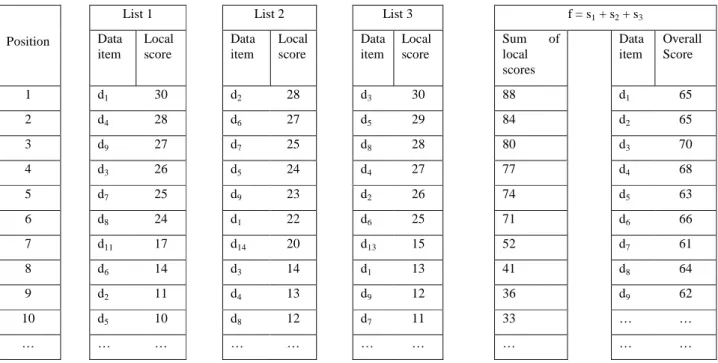
As an example, consider the database (i.e. the three sorted lists) shown in Figure 2, and suppose k=3 and the scoring function computes the sum of the local scores. If we apply BPA on this example, it stops at position 7, so it does 7∗3 sorted accesses and 7∗3∗2 random accesses. Thus, the total number of accesses done by BPA is nbpa = 63. If we apply BPA2, it does direct access to

positions 1, 2, 3 and 7 in all lists, so a total of 4∗3 direct accesses and 4∗3∗2 random accesses. Thus, the total number of accesses done by BPA2 is nbpa2 = 36. Therefore, we have nbpa≈ 2

∗

nbpa2.

5.2 Managing Best Positions

After each sorted/direct/random access to a list, the owner of the list needs to determine the best position. A simple method for managing the best positions is to maintain the seen positions in a set. Then finding the best position is done by scanning the set and for each position p, verifying if all positions which are less than p belong to the set. This method is not efficient because finding the best position is done in O(u2) where u is the number of seen positions. Note that in the worst case, u can be equal to n, i.e. the number of data items in the list. In this section, we propose two efficient techniques for managing best positions: Bit array, and B+tree.

5.2.1 Bit Array

In this approach, to know the positions which are seen, each list owner uses an array of n bits where n is the size of the sorted list. Initially all bits of the array are set to 0. There is a variable bp which points to the best position. Initially bp is set to 1. Let Bi be

the bit array which is used by the owner of list Li. After doing an

access to a data item that is at position j in Li, the following

instructions are done by the list owner for determining the new best position:

Bi[j] := 1;

While ((bp < n) and (Bi[bp + 1] = 1)) do

bp := bp + 1;

The total time needed for determining the best positions during the execution of the top-k query is O(n), i.e. bp can be incremented up to n. Let u be the total number of accesses to Li

during the execution of the query, then the average time for determining the best position after each access is O(n/u). The space needed for this approach is an array of n bits plus a variable, which is typically very small.

5.2.2 B

+

tree

In this approach, each list owner uses a B+tree for maintaining the seen positions. B+tree is a balanced tree, which is widely used for efficient data storage and retrieval in databases. In a B+tree, all data is saved in the leaves, and the leaf nodes are at the same level, so any operation of insert/delete/lookup is logarithmic in the number of data items. The leaf nodes are also linked together as a linked list. Let c be a cell of the linked list, i.e. a leaf of the B+tree, then there is a pointer c.next that points to the next cell of the linked list. Let c.element be a variable that maintains the data in c. Let BTi be the B

+

tree which the owner of list Li uses for

maintaining the seen positions of Li. The list owner also uses a

pointer bp that points to the cell, i.e. leaf of BTi, which maintains

the seen position which is the best position. After an access to a position p in Li, the list owner adds p to BTi. Then, it performs the

following instructions to determine the new best position:

While ((bp.next ≠ null) and (bp.next.element

= bp.element + 1)) do bp := bp.next;

List 1 List 2 List 3 f = s1 + s2 + s3

Position Data item Local score Data item Local score Data item Local score Sum of local scores Data item Overall Score 1 d1 30 d2 28 d3 30 88 d1 65 2 d4 28 d6 27 d5 29 84 d2 65 3 d9 27 d7 25 d8 28 80 d3 70 4 d3 26 d5 24 d4 27 77 d4 68 5 d7 25 d9 23 d2 26 74 d5 63 6 d8 24 d1 22 d6 25 71 d6 66 7 d11 17 d14 20 d13 15 52 d7 61 8 d6 14 d3 14 d1 13 41 d8 64 9 d2 11 d4 13 d9 12 36 d9 62 10 d5 10 d8 12 d7 11 33 … … … … … …

(9)

The above instructions assure that the pointer bp points always to the cell which maintains the best position. Let u be the total number of accesses to the list Li during the execution of the query,

then the total time for determining the best positions is O(u), i.e. in the worst case bp moves from the head to the end of the linked list. Thus, the average time per access is O(1). The time needed for adding a seen position to the B+tree is O(log u). Therefore, with the B+tree approach, the average time for storing a seen position and determining the best position is O(log u). For the Bit array approach, this time is O(n/u) where n is the size of the sorted list. If n is much greater than u, i.e. n≥ c∗ (u ∗ log u) where c is a constant that depends on the B+_{tree implementation, then the}

B+tree approach is more efficient than the Bit array approach. The space needed for the B+tree approach is O(u) but is not usually as compact as Bit array.

6. PERFORMANCE EVALUATION

In the previous sections, we analytically compared our algorithms with TA, i.e. BPA directly and BPA2 indirectly. In this section, we compare these three algorithms through experimentation over randomly generated databases. The rest of this section is organized as follows. We first describe our experimental setup. Then, we compare the performance of our algorithms with TA by varying experimental parameters such as the number of lists, i.e. m, the number of top data items requested, i.e. k, and the number of data items of each list, i.e. n. Finally, we summarize the performance results.

6.1 Experimental Setup

We implemented TA, BPA and BPA2 in Java. To evaluate our algorithms, we tested them over both independent and correlated databases, thus covering all practical cases. The independent databases are uniform and Gaussian databases generated using the two main probability distributions (i.e. uniform and Gaussian). With Uniform database, the positions of a data item in any two lists are independent of each other. To generate this database, the scores of the data items in each list are generated using a uniform random generator, and then the list is sorted. This is our default setting. With Gaussian database, the positions of a data item in any two lists are also independent of each other. To generate this database, the scores of the data items in each list are Gaussian random numbers with a mean of 0 and a standard deviation of 1. In addition to these independent databases, we also use correlated databases, i.e. databases where the positions of a data item in the lists are correlated. We use this type of database for taking into account the applications where there are correlations among the positions of a data item in different lists. In real-world applications, there are usually such correlations [23]. Inspired from [23], we use a correlation parameter α (0 ≤α ≤ 1), and we generate the correlated databases as follows. For the first list, we randomly select the position of data items. Let p1 be the position

of a data item in the first list, then for each list Li (2 ≤ i ≤ m) we

generate a random number r in interval [1 .. n∗α] where n is the number of data items, and we put the data item at a position p whose distance from p1 is r. If p is not free, i.e. occupied

previously by another data item, we put the data item at the free position closest to p. By controlling the value of α, we create databases with stronger or weaker correlations. After setting the positions of all data items in all lists, we generate the scores of the

data items in each list in such a way that they follow the Zipf law [29] with the Zipf parameter θ = 0.7. The Zipf law states that the score of an item in a ranked list is inversely proportional to its rank (position) in the list. It is commonly observed in many kinds of phenomena, e.g. the frequency of words in a corpus of natural language utterances.

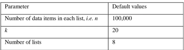
Our default settings for different experimental parameters are shown in Table 1. In our tests, the default number of data items in each list is 100,000. Typically, users are interested in a small number of top answers, thus unless otherwise specified we set k=20. Like many previous works on top-k query processing, e.g. [8], we use a scoring function that computes the sum of the local scores. In most of our tests, the number of lists, i.e. m, is a varying parameter. When m is a constant, we set it to 8 which is rather small but quite sufficient to show significant performance gains of our algorithms. Note that, in some important applications such as network monitoring [8], m can be much higher.

Table 1. Default setting of experimental parameters

Parameter Default values

Number of data items in each list, i.e. n 100,000

k 20

Number of lists 8

To evaluate the performance of the algorithms, we measure the following metrics.

1) Execution cost. As defined in Section 2, the execution cost is

computed as c = as∗cs + ar∗cr where as is the number of sorted

accesses that an algorithm does during execution, ar is the number

of random accesses, cs is the cost of a sorted access, and cr is the

cost of a random access. For the BPA2 algorithm, we consider each direct access equivalent to a random access. For each sorted access we consider one unit of cost, i.e. we set cs = 1. For the cost

of each random access, we set cr = log n where n is the number of

data items, i.e. we assume that there is an index on data items such that each entry of index points to the position of data item in the lists. The execution time which we consider here is a good metric for comparing the performance of the algorithms in a centralized system. For distributed systems, we use the next metric.

2) Number of accesses. This metric measures the total number of

accesses to the lists done by an algorithm during execution. It involves the sorted, direct and random accesses. In distributed systems, particularly in the cases where message size is small (which is the case of our algorithms), the main cost factor is the number of messages communicated between nodes. The number of messages, which our algorithms (and TA) communicate between the query originator and list owners in a distributed system, is proportional to the number of accesses done to the lists. Thus, the number of accesses is a good metric for comparing the performance of the algorithms in distributed systems. For TA and BPA, the number of accesses is also a good indicator of their stopping position under sorted access, i.e. the number of accesses is m2 multiplied by the stopping position.

3) Response time. This is the total time (in millisecond) that an

algorithm takes for finding the top-k data items. We conducted our experiments on a machine with a 2.4 GHz Intel Pentium 4

(10)

processor and 2GB memory. In the code of BPA and BPA2, the best positions are managed using the Bit Array approach which is simpler than the B+-tree approach.

6.2 Performance Results

6.2.1 Effect of the number of lists

In this section, we compare the performance of our algorithms with TA over the three database types while varying the number of lists.

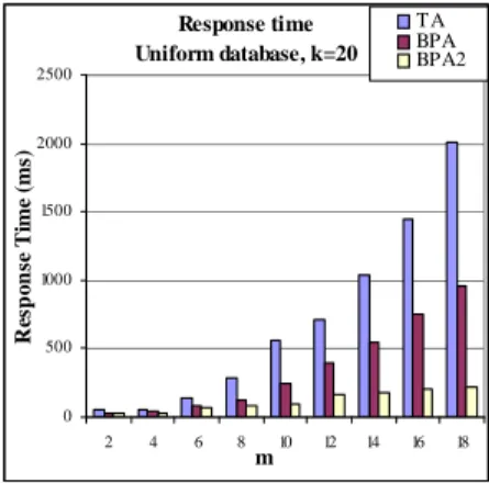
Over the uniform database, with the number of lists increasing up to 18 and the other parameters set as in Table 1, Figures 3, 4 and 5

Execution cost Uniform database, k=20 0 10000000 20000000 30000000 40000000 50000000 60000000 2 4 6 8 10 12 14 16 18 m E x ec u ti o n C o st T A BPA BPA2 Number of accesses Uniform database, k=20 0 500000 1000000 1500000 2000000 2500000 3000000 3500000 4000000 2 4 6 8 10 12 14 16 18 m N u m b er o f A cc es se s T A BPA BPA2 Response time Uniform database, k=20 0 500 1000 1500 2000 2500 2 4 6 8 10 12 14 16 18 m R es p o n se T im e (m s) TA BPA BPA2

Figure 3. Execution cost vs. number of

lists over uniform database

Figure 4. Number of accesses vs. number

of lists over uniform database

Figure 5. Response time vs. number of

lists over uniform database

Execution cost Gaussian database, k=20 0 10000000 20000000 30000000 40000000 50000000 60000000 2 4 6 8 10 12 14 16 18 m Ex ec u ti o n C o st T A BPA BPA2 Number of accesses Gaussian database, k=20 0 500000 1000000 1500000 2000000 2500000 3000000 3500000 4000000 2 4 6 8 10 12 14 16 18 m N u m b er o f A cc es se s T A BPA BPA2 Response time Gaussian database, k=20 0 400 800 1200 1600 2000 2 4 6 8 10 12 14 16 18 m R es p o n se T im e (m s) T A BP A BP A2

lists over Gaussian database

Figure 7. Number of accesses vs. number

of lists over Gaussian database

Figure 8. Response time vs. number of

lists over Gaussian database

Execution cost Correlated database, alfa=0.001, k=20

0 2 000 0 4 000 0 6 000 0 8 000 0 10 000 0 12 000 0 14 000 0 16 000 0 18 000 0 2 4 6 8 10 12 14 16 18 m E x ec u ti o n C o st T A BP A BP A2 Execution cost Correlated database , alfa=0.01, k=20

0 2 00 0 0 0 4 00 0 0 0 6 00 0 0 0 8 00 0 0 0 10 00 0 0 0 12 00 0 0 0 2 4 6 8 10 12 14 16 18 m E x ec u ti o n C o st T A BP A BP A2 Execution cost Correlated database, alfa=0.1, k=20

0 10 000 00 20 000 00 30 000 00 40 000 00 50 000 00 60 000 00 70 000 00 80 000 00 90 000 00 2 4 6 8 10 12 14 16 18 m E x ec u ti o n C o st T A BP A BP A2

lists over correlated database with α=0.001

lists over correlated database with α=0.01

(11)

show the results measuring execution cost, number of accesses, and response time, respectively. The execution cost of BPA is much better than that of TA; it outperforms TA by a factor of approximately (m+6)/8 for m>2. BPA2 is the strongest performer; it outperforms TA by a factor of approximately (m+1)/2 for m>2. On the second metric, i.e. number of accesses, the results are similar to those on execution cost. However, BPA2 outperforms TA by a factor which is (a little) higher than that for execution cost, i.e. about 1/m higher. The reason is that for measuring execution cost, we assume an expensive cost (i.e. log n units) for direct accesses which are done by BPA2. On response time, BPA2 (and BPA) outperforms TA by a factor which is a little lower than that on execution cost, just because of the time they need for managing the best positions.

Over the Gaussian database, with the number of lists increasing up to 18 and the other parameters set as in Table 1, Figures 6, 7 and 8 show the results for execution cost, number of accesses, and response time respectively. Over the Gaussian database, the performance of the three algorithms is a little better than their performance over the uniform database. BPA and BPA2 do much better than TA, and they outperform it by a factor close to that over the uniform database.

Overall, the performance results on the three metrics are qualitatively similar, in particular on execution cost and number of accesses. Thus, in the rest of this paper, we only report the results on execution cost.

Figures 9, 10 and 11 show the execution cost of the algorithms over three correlated databases with correlation parameter α set to 0.001, 0.01 and 0.1 respectively, and the other parameters set as in Table 1. Over these databases, the performance of the three algorithms is much better than that over Gaussian and uniform databases. In fact, the more correlated is the database; the lower is the execution cost of all three algorithms. The reason is that in a highly correlated database, the top-k data items are distributed over low positions of the lists, so the algorithms do not need to go much down in the lists, and they stop soon. However, due to their efficient stopping mechanism, BPA and BPA2 stop much sooner than TA.

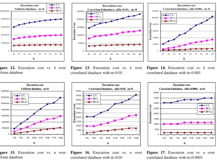
6.2.2 Effect of k

In this section, we study the effect of k, i.e. the number of top data items requested, on performance. Figure 12 shows how execution cost increases over the uniform database, with increasing k up to 100, and the other parameters set as in Table 1. The execution cost of all three algorithms increases with k because more data items are needed to be returned in order to obtain the top-k data items. However, the increase is very small. The reason is that over the uniform database, when an algorithm (i.e. any of the three algorithms) stops its execution for a top-k query, with a high probability, it has seen also the (k + 1)th data item. Thus, with a high probability, it stops at the same position for a top-(k+1) query. Executi on cost Uniform database, m=8 0 2 00 00 0 0 4 00 00 0 0 6 00 00 0 0 8 00 00 0 0 10 00 00 0 0 10 2 0 30 40 5 0 6 0 7 0 8 0 90 10 0 k E x ec u ti o n C o st T A BP A BP A2 Execution cos t Correlated databas e, alfa=0 .0 1 , m=8

0 50000 100000 150000 200000 250000 10 20 30 40 50 60 70 80 90 100 k E x ec u ti o n C o st T A BP A BP A2

Exe cution cost Corre late d database , alfa=0.001, m=8

0 2 00 00 4 00 00 6 00 00 8 00 00 10 00 00 12 00 00 10 20 3 0 4 0 50 60 7 0 8 0 90 100 k E x ec u ti o n C o st T A BP A BP A2

Figure 12. Execution cost vs. k over

uniform database

correlated database with α=0.01

Execution cost Uniform database, m=8 0 2000000 4000000 6000000 8000000 10000000 12000000 14000000 25K 50K 75K 100K 125K 150K 175K 200K n E x ec u ti o n C o st TA BPA BPA2 Execution cost Correlated database, alfa=0.01, m=8

0 5000 10000 15000 20000 25000 30000 35000 40000 45000 50000 25K 50K 75K 100K 125K 150K 175K 200K n E x ec u ti o n C o st TA BPA BPA2 Execution cost, Correlated database, alfa=0.0001, m=8

0 5000 10000 15000 20000 25000 30000 35000 40000 25K 50K 75K 100K 125K 150K 175K 200K n E x ec u ti o n C o st TA BPA BPA2

Figure 15. Execution cost vs. n over

uniform database

(12)

Figures 13 and 14 show how execution cost increases with increasing k over two correlated databases with correlation parameter set to α=0.01 and α=0.001 respectively, and the other parameters set as in Table 1. For the database with α=0.01, i.e. the one which is less correlated, the impact of k is smaller. The reason is that when we run one of the three algorithms over a database with low correlation, it sees a lot of data items before stopping its execution. Thus, when it stops at a position for a top-k query, there is a high probability that it stops at the same position for a top-(k + 1) query. But, for a highly correlated database, this probability is lower because the algorithm sees a small number of data items before stopping its execution.

6.2.3 Effect of the number of data items

In this section, we vary the number of data items in each list, i.e. n, and investigate its effect on execution cost. Figure 15 shows how execution cost increases over the uniform database with increasing n up to 200,000, and with the other parameters set as in Table 1. Increasing n has a considerable impact on the performance of the three algorithms over a uniform database. The reason is that when we enlarge the lists and generate uniform random data for them, the top-k data items are distributed over higher positions in the list.

Figures 16 and 17 show how execution cost increases with increasing n over two correlated databases with correlation parameter set to α=0.01 and α=0.001 respectively, and the other parameters set as in Table 1. The results show that n has a smaller impact on a highly correlated database rather than a database with a low correlation.

6.2.4 Concluding remarks

The performance results show that, over all test databases and wrt all the metrics, the performance of our algorithms is much better than that of TA. For example, they show that wrt execution cost, BPA and BPA2 outperform TA by a factor of approximately (m+6)/8 and (m+1)/2 for m>2. Thus, as m increases, the performance gains of our algorithms versus TA increase significantly.

7. RELATED WORK

Efficient processing of top-k queries is both an important and hard problem that is still receiving much attention. A first important paper is [13] which models the general problem of answering top-k queries using lists of data items sorted by their local scores and proposes a simple, yet efficient algorithm, Fagin’s algorithm (FA), that works on sorted lists. The most efficient algorithm over sorted lists is the TA algorithm which was proposed by several groups4 [14] [16] [25]. TA is simple, elegant and efficient [15] and provides a significant performance improvement over FA. We already discussed much TA in this paper. However, because of its stopping mechanism (based on the last seen scores under sorted access), TA can still perform useless work (see Section 3). The fundamental differences between BPA and TA are the following. BPA takes into account the positions and scores of the seen data whereas TA only takes into account their scores. Using

4

The second author of [14] first defined TA and compared it with FA at the University of Maryland in the Fall of 1997.

information about the position of the seen data, BPA develops a more intelligent stopping mechanism that allows choosing a much better time to stop (such choice is correct as proved in Lemma 1). This allows BPA to gain much reduction in the number of sorted accesses and thus much reduction in the number of random accesses. Even if TA were keeping track of all seen data items, it could not stop at a smaller position under sorted access, because its threshold does not allow it.

Several TA-style algorithms, i.e. extensions of TA, have been proposed for processing top-k queries in distributed environments, e.g. [6] [7] [9] [12] [23]. Overall, most of the TA-style algorithms focus on extending TA with the objective of minimizing communication cost of top-k query processing in distributed systems. They could as well use our algorithms to increase performance. To do so, all they need to do is to manage the best positions at list owners as in BPA2, and then use BPA2's stopping mechanism. This would significantly reduce the accesses to the lists and yield significant performance gains.

The Three Phase Uniform Threshold (TPUT) [8] is an efficient algorithm to answer top-k queries in distributed systems. The algorithm reduces communication cost by pruning away ineligible data items and restricting the number of round-trip messages between the query originator and the other nodes. The simulation results show that TPUT can reduce communication cost by one to two orders of magnitude compared with an algorithm which is a direct adaptation of TA for distributed systems [8]. However, there are many databases over which TPUT is not instance optimal [8]. For example, if one of the lists has n data items with a fixed value that is just over the threshold of TPUT, then all data items must be retrieved by the query originator, while a more adaptive algorithm might avoid retrieving all n data items. Instead, our algorithms are instance optimal over all databases and can reduce the cost (m-1) orders of magnitude compared to TA.

8. CONCLUSION

The most efficient algorithm proposed so far for answering top-k queries over sorted lists is the Threshold Algorithm (TA). However, TA may still incur a lot of useless accesses to the lists. In this paper, we proposed two algorithms which stop much sooner and thus are more efficient than TA.

First, we proposed the BPA algorithm whose stopping mechanism takes into account the seen positions in the lists. For any database instance (i.e. set of sorted lists), we proved that BPA stops at least as early as TA. We showed that the number of sorted/random accesses done by BPA is always less than or equal to that of TA, and thus its execution cost is never higher than TA. We also showed that the number of sorted/random accesses done by BPA can be (m-1) times lower than that of TA. Thus, its execution cost can be (m-1) times lower than that of TA. We showed that BPA is instance optimal over all databases, and its optimality ratio is better than or equal to that of TA.

Second, based on BPA, we proposed the BPA2 algorithm which is much more efficient than BPA. In addition to its efficient stopping mechanism, BPA2 avoids re-accessing data items via sorted and random access, without having to keep data at the query originator. We showed that the number of accesses to the lists done by BPA2 can be about (m-1) times lower than that of BPA.