Titre:
Title:
Modelling of a water-to-air variable capacity ground-source heat pump
Auteurs:
Authors: Samuel Bouheret et Michel Bernier
Date: 2018
Type: Article de revue / Journal article
Référence:
Citation:
Bouheret, Samuel et Bernier, Michel (2018). Modelling of a water-to-air variable capacity ground-source heat pump. Journal of Building Performance Simulation, p. 1-11. doi:10.1080/19401493.2017.1332686
Document en libre accès dans PolyPublie
Open Access document in PolyPublie
URL de PolyPublie:
PolyPublie URL: http://publications.polymtl.ca/2641/
Version: Version finale avant publication / Accepted versionRévisé par les pairs / Refereed Conditions d’utilisation:
Terms of Use: CC BY-NC-ND
Document publié chez l’éditeur officiel
Document issued by the official publisher
Titre de la revue:
Journal Title: Journal of Building Performance Simulation
Maison d’édition:
Publisher: Taylor & Francis
URL officiel:
Official URL: http://dx.doi.org/10.1080/19401493.2017.1332686
Mention légale:
Legal notice:
This is an Accepted Manuscript of an article published by Taylor & Francis in Journal of Building Performance Simulation on 2017-06-15, available online:
http://www.tandfonline.com/10.1080/19401493.2017.1332686.
Ce fichier a été téléchargé à partir de PolyPublie, le dépôt institutionnel de Polytechnique Montréal
This file has been downloaded from PolyPublie, the institutional repository of Polytechnique Montréal
1
Modelling of a water-to-air variable capacity
ground source heat pump
by
Samuel Bouheret and
Michel Bernier1
Polytechnique Montréal Département de génie mécanique
2500 chemin de Polytechnique Montréal, Canada, H3T 1J4
Final version accepted for publication in the Journal of Building Performance Simulation
April 2017
2
Modelling of a water-to-air variable capacity
ground-source heat pump
ABSTRACT
The present work aims at presenting the development of a performance-based model of a water-to-air variable capacity ground-source heat pump. The main challenge is to apply the recommended control strategy to vary the speed of the compressor for each mode of operation and to be able to switch from one mode to the other. A series of verification tests tend to confirm that the speed control strategy has been correctly implemented. The proposed model is used in annual simulations of a residential system equipped with a variable capacity ground-source heat pump. In this case, the seasonal performance factor (SPF = ratio of the annual energy requirement for heating, cooling and DHW over the annual total energy consumption) is 3.64. The corresponding value for a conventional system composed of a single capacity heat pump operating in on-off mode and a separate electric DHW tank is 2.60.
3
1. Introduction and literature review
Ground-source heat pumps can provide space conditioning and domestic hot water with a high level of energy efficiency (Simon et al. 2016). Since most of them are sized to meet the annual peak building loads, they need to operate at partial capacity most of the time. The most common way of varying the capacity is with intermittent heat pump operation. The duration of the off period is adjusted so that, on average, the heat pump capacity is equal to the load. Variable capacity ground-source heat pumps, however, can provide a variable output which leads to more stable space temperatures and reduced cycling losses associated with part load operation. Furthermore, some have two reversing valves which enable multiple modes of operation including the production of domestic hot water (DHW) with either the ground or the house as the heat source. These heat pumps offer significant improvements over conventional heat pumps. However, very few researchers have developed detailed models that could be used in simulation studies to quantify their energy benefits.
The intermittent mode of operation of conventional heat pumps comes at the price of reduced thermal comfort, equipment lifetime and energy efficiency (Bagarella, Lazzarin, and Noro, 2016). Among alternative methods of control, Zhao et al. (2003) showed that varying the compressor speed is probably the most interesting one. It typically shows better performances at part load due to reduced temperature difference in the heat exchangers and improved compressor efficiency (Madani et al, 2010). Karlsson and Fahlén (2007a) compared on-off operated and variable capacity heat pumps. In order to maintain the same mean temperature over one cycle, on-off heat pumps have to deliver heat during the on period at a higher temperature than variable capacity heat pumps, which leads to a better coefficient of performance (COP) for variable capacity machines. According to Madani, Claesson and Lundqvist (2011), sizing the heat pump to face a small fraction (under 66%) of peak load to reduce compressor cycling results in an increase in auxiliary energy consumption (electric or gas), which degrades the overall seasonal performance factor. Since they operate over a wide operating range, variable capacity heat pumps can cover a large share of the building load while limiting cycling at partial load (Bagarella, Lazzarin,
4 and Noro, 2016). Numerous studies have focused on evaluating the benefits of variable capacity, the conclusions of which sometimes point out different results depending on a wide set of parameters. The cycling losses and dynamic effects, the use of variable or fixed speed circulating pumps and fans, and the sizing of on-off heat pumps relative to the building peak load seem to all affect the conclusions of the studies on variable capacity heat pumps. For example, in their study, Karlsson and Fahlén (2007a) neglect cycling losses and dynamic effects and show no benefit from variable capacity, but demonstrate that secondary fluid flows have to be varied according to the refrigerant flow rate to achieve maximum efficiency, thus requiring variable speed circulating pump or fan. Karlsson and Fahlén (2007b) showed that comparisons on a steady-state basis overestimate the performances of fixed speed systems, thus do not fully display the benefits of variable capacity. Corberán (2016) also indicates that compressor manufacturers usually optimize their products for higher pressure ratios than the ones commonly met in a variable capacity heat pump. He points out that higher performances could be reached if the compressor was selected for low pressure ratios typical of variable capacity ground-source heat pumps. Del Col et al. (2012) mention that the most important parameter in a variable capacity heat pump is the motor type: switching from an asynchronous to a brushless motor can lead to an improvement of approximately 20% in the COP value.
Several approaches can be found in the literature on heat pump modelling. They range from empirical, equation-fit models to detailed physical models. Empirical or equation-fit models, such as the one from Nyika et al. (2014), are based on experimental or manufacturer’s data and treat the heat pump as a “black box”, without describing each component individually. Other models like the one developed by Ndiaye and Bernier (2012a, 2012b) adopt a distributed approach, where each component is modeled in detail, and then linked together. This later approach requires an accurate knowledge of the heat pump geometry which is usually not readily available. Blervaque et al. (2016) suggest to classify modelling approaches according to two criteria: their degree of physical detail (empirical, simple thermodynamic models or detailed physical models) and their degree of dynamic consideration (quasi-static or dynamic models).
5 Work has been done on an earlier version of the heat pump modeled in the present study (Rice et al. 2013 ; Baxter et al. 2013). In these studies, the experimentally validated heat pump design model (HPDM) of Oak Ridge National Laboratory was used to generate equipment performance maps for each operation mode as a function of all independent variables. These maps were then used in TRNSYS with a custom model and thermostat control logic. The resulting model was used in annual simulations with a 3-min time step for five US climates. These simulations showed that variable capacity heat pumps used for space conditioning and DHW production use 52 to 59% less energy than a system composed of an air source heat pump and an electric water heater.
The TRNSYS and TESS standard libraries (Klein et al. 2014 ; TESS 2012) include single and dual speed ground source heat pump models. However, these models are not adapted to variable capacity modelling.
The present work aims at presenting the development of a water-to-air variable capacity ground-source heat pump model. The model is first described, followed by a series of verification tests to check the model for each operating mode. Finally, an application section demonstrates the use of the proposed model in annual simulations and shows the energy saving potential of such heat pumps when compared to conventional single capacity heat pumps.
2. Heat pump operation and data
The model developed in this study corresponds to a specific heat pump (Climate Master, 2014). This manufacturer offers two heat pumps of different capacities; the QE930 is modeled in the present study. However, other variable capacity heat pumps could also be easily modeled using the same approach by modifying the performance maps files. Model QE930 has nominal rated capacities of 7.0 and 8.8 kW in cooling and heating, respectively. The model is based on performance maps obtained for steady-state operation, thus placing it in the first category proposed by Blervaque et al. (2016): quasi-static, empirical approach. Even though these data are valid for steady-state operation, they can accurately describe
6 the heat pump performance in dynamic operation, as shown by Waddicor et al. (2016) and Corberán et al. (2013).
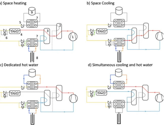
The heat pump is a residential size ground-source heat pump with variable-speed compressor, pumps and fan which are all equipped with high-efficiency permanent magnet brushless motor. As shown in Figure 1, with two reversing valves, the heat pump can operate in four distinct modes: space heating, dedicated space cooling, dedicated DHW production and simultaneous space cooling and DHW production. The first three modes use the ground heat exchanger (GHX) as a heat source or sink, whereas the fourth uses heat from the building to provide hot water.
An excerpt from the manufacturers’ data in heating mode is presented in Table 1. This table only includes two values of entering water temperature (𝐸𝑊𝑇) and air flow rate, and a limited number of heating capacities. The complete table includes seven different 𝐸𝑊𝑇, three different air flow rates and five different heating capacities.
As shown in Table 1, the heat pump capacity can be varied from 2.6 to 8.8 kW. The heat pump is able to maintain its capacity over a wide range of 𝐸𝑊𝑇 (i.e. the return temperature from the GHX), source ∆𝑇, and air flow rate. It does so by varying the compressor frequency from 25 to 130 Hz depending on the required capacity. In Table 1, fan power is included but the power of the GHX pump and the hot water tank circulator pump are excluded. As shown by Madani, Claesson and Lundqvist (2011), pumping power can be responsible for a large share of the energy consumption in variable capacity heat pumps,
Table 1 Excerpt from manufacturer’s data (Heating mode)
Entering water temperature ( 𝐸𝑊𝑇) (°C) Source T (°C) Air flow rate (L/s per kW of HC)* Heating capacity
(kW) Power input (in kW) and (COP)
Compressor Frequency (Hz) -1.1 6.7 40.0 2.6 5.3 8.8 0.95 (2.8) 1.68 (3.1) 3.07 (2.8) 54 90 130 67.1 2.6 5.3 8.8 0.75 (3.5) 1.46 (3.6) 2.92 (3.0) 50 87 130 3.3 40.0 2.6 5.3 8.8 0.89 (3.0) 1.55 (3.4) 2.90 (3.0) 46 83 123 67.1 2.6 5.3 8.8 0.68 (3.9) 1.31 (4.0) 2.68 (3.3) 45 83 121 32.2 6.7 40.0 2.6 5.3 8.8 0.44 (6.5) 0.74 (7.1) 1.23 (7.2) 25 43 66 67.1 2.6 5.3 8.8 0.32 (10.2) 0.55 (9.5) 1.09 (8.1) 26 40 62 3.3 40.0 2.6 5.3 8.8 0.42 (7.1) 0.70 (7.6) 1.13 (7.8) 25 41 63 67.1 2.6 5.3 8.8 0.29 (12.0) 0.50 (10.5) 0.99 (8.9) 25 41 64 * 40.0 and 67.1 L/s per kW of heating capacity correspond to 300 and 500 CFM /ton
7 1) Compressor. 2) 1st reversing valve. 3) 2nd reversing valve. 4) Micro channel heat exchanger. 5) Check valves.
6) Electronic expansion valves. 7) Brazed plate heat exchangers. 8) Borehole. 9) Hot water tank.
Fig. 1. Refrigerant flow for the 4 operating modes.
High pressure vapor High pressure liquid Low pressure liquid
8 since they achieve longer operating time than on-off heat pumps. It is interesting to note the COP variation with compressor frequency. Taking the first line of the table as an example, the COP is equal to 2.8, 3.1, and 2.8 for compressor frequencies of 54, 90, and 130 Hz, respectively. This typical behavior indicates that the COP reaches a peak near the mid-point of the compressor frequency range.
Three other performance maps are available from the manufacturer to cover the other three operating modes. These maps will not be presented here as they exhibit a format similar to Table 1. For space cooling, the heat pump can vary the total (sensible + latent) capacity from 2.6 to 8.8 kW. When space cooling and DHW are provided simultaneously, it is still possible to vary the compressor frequency to change the total cooling capacity from 2.6 to 8.8 kW. This “heat” is transferred to the DHW tank using the refrigeration cycle by bypassing the GHX. The compressor requires 0.8 and 3.5 kW of power (for a returning hot water tank temperature of ≈ 43 °C) for total cooling capacities of 2.6 and 8.8 kW, respectively. Thus, the DHW capacity is approximately 3.4 and 12.3 kW in this mode. Finally, when the heat pump provides dedicated DHW production, the water heating capacity varies from about 3.8 to 4.8 kW depending on whether the returning hot water tank temperature is high (≈ 50 °C) or low (≈ 20 °C).
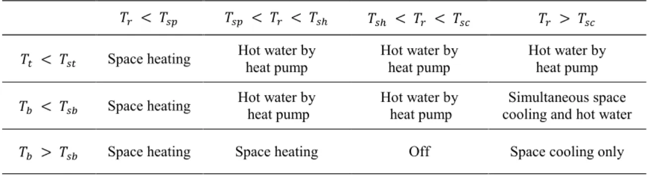
The manufacturer recommends to control this heat pump using a PI-type controller as shown in Figure 2. The controller has two main roles: determining the required operating mode (heating, cooling, DHW production or simultaneous cooling and DHW production), and controlling the compressor frequency for the current operating mode. The controller also commands the flow rate at which the GHX pump and hot water tank circulator as well as the fan need to operate. The water flow rates are calculated based on the source and DHW ∆𝑇𝑠 and the air flow rate per unit capacity set by the user. The controlled temperatures are presented in Figure 2, and the controller logic is summarized in Table 2. The controller determines the required operation mode based on the top and bottom hot water tank temperatures, 𝑇𝑡, and 𝑇𝑏 , as well as the house temperature, 𝑇𝑟. The values of
9 of the hot water tank, respectively. A 2 K dead band is applied to avoid control instabilities and too frequent mode-to-mode switching.
The following control logic is used: priority is given to DHW production over heating, unless the space temperature has dropped under a user-defined limit (𝑇𝑠𝑝), at which point
heating is granted priority. Thus, heating mode is active when space temperature is under the priority limit or when hot water is not needed. Dedicated DHW mode is active when the bottom tank temperature is below 𝑇𝑠𝑏 but no space cooling is necessary; simultaneous
cooling and hot water production is active otherwise. The dedicated cooling mode is active when cooling is needed and the bottom tank temperature is greater than 𝑇𝑠𝑏. Finally, if the
top tank temperature is below 𝑇𝑠𝑡 , the top electric water heating element is energized.
Fig. 2. Schematic representation of the operation of a variable capacity ground-source heat pump for space conditioning and domestic hot water production.
10 Once the operating mode is known, the controller determines the required compressor frequency. For DHW production, compressor frequency is determined based on the returning fluid temperature from the GHX, the returning water temperature from the bottom of the hot water tank and the ∆𝑇𝑠 set by the user on both the GHX and hot water tank side. For other modes, a proportional-integral (PI) action is used. The PI monitors space temperature and adjusts the compressor frequency accordingly.
There are minimum and maximum operating frequency limits for the compressor. As explained by Corberan (2016), the compressor speed is limited by lubrication issues: at low speed, the sealant effect produced by the lubricant disappears, while at high speed, friction can produce high temperature that can cause the lubrication to fail. For small loads, the heat pump reaches its minimum operating frequency and has to be switched on-off to control capacity. This is regulated by the 2 K dead bands of the thermostats used to determine the correct operating mode. If the compressor stopped because of insufficient modulating capacity, it is likely to have to operate in intermittent mode until the load increases again. When starting again after a stop, it is desirable for the heat pump to run at its minimal capacity, so that it does not have to stop again too soon (anti-short-cycling time are typically in the range of a few minutes). For this reason, the 1 K temperature drop (or rise) causing the thermostat to switch has to correspond to the minimal possible frequency (25 Hz), so a 25 Hz/K gain is applied to the PI controller. A 0.25 h integral time constant
Table 2 : Controller logic
𝑇𝑟 < 𝑇𝑠𝑝 𝑇𝑠𝑝 < 𝑇𝑟 < 𝑇𝑠ℎ 𝑇𝑠ℎ < 𝑇𝑟 < 𝑇𝑠𝑐 𝑇𝑟 > 𝑇𝑠𝑐
𝑇𝑡 < 𝑇𝑠𝑡 Space heating Hot water by heat pump Hot water by heat pump Hot water by heat pump
𝑇𝑏 < 𝑇𝑠𝑏 Space heating Hot water by heat pump Hot water by heat pump cooling and hot water Simultaneous space
𝑇𝑏 > 𝑇𝑠𝑏 Space heating Space heating Off Space cooling only
11 has been found to correctly maintain set-point while avoiding excessive overshoot during transient phases. When the load increases again, heat pump capacity is sufficient to keep the controlled temperature within the dead band, in which case the heat pump operates in variable capacity mode.
3. Heat pump model
The heat pump model described in this section is to be used in the TRNSYS simulation environment (Klein et al. 2014). Figure 3 shows a subset of the final heat pump model where only the space heating calculations are shown; similar assemblies are required for the other three modes of operation. A distributed approach, where existing TRNSYS Types are grouped together to form the heat pump model, is used instead of developing an entirely new Type.
Space heating subset of the heat pump model Three other subsets of the
heat pump model
Heat pump model
Space heating subset of the heat pump model Three other subsets of the
heat pump model
Heat pump model
Figure 3 Subset of the heat pump model showing the various Types involved in the space heating calculations
Overall, the heat pump model includes the controller logic (Type 40), three PI controllers (Type 23), a multitude of performance maps accessed through multi-dimensional data interpolation Types (Type 581), and calculators to enter simple algebraic equations. As shown in Table 1, performance maps give the required frequency as a function of capacity.
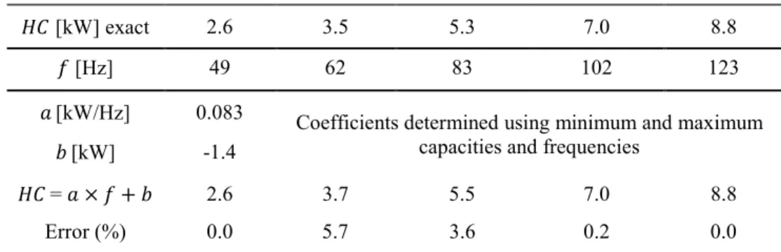
12 However, in reality, the compressor runs at the frequency determined by the controller and the capacity varies according to that frequency. It would have been preferable to have performance maps with capacity given as a function of frequency. To take this behavior into account, a relationship between capacity and frequency is determined, then the capacity corresponding to the frequency defined by the controller is used to read the performance data. Compressor frequency varies almost linearly with capacity. Thus, only two pairs of capacity–frequency data are needed to evaluate the linear relationship. These two values are determined based on frequency and capacity limits: in heating, the capacity is always limited between 2.6 and 8.8 kW, and the minimum and maximum frequencies allowed vary according to operating conditions (see Table 1). Knowing the frequency corresponding to 2.6 and 8.8 kW, it is possible to determine the linear relationship between heating capacity (𝐻𝐶) and frequency (𝑓) (i.e. 𝐻𝐶 = 𝑎 × 𝑓 + 𝑏). A data table of heating frequency limits is built which outputs minimum and maximum frequencies and capacities for each operating condition and for each space conditioning mode. Table 3 shows how the coefficients 𝑎 and 𝑏 are determined for a specific condition. The last line of this table also shows the range of error (in %) between the real 𝐻𝐶 and the one estimated based on the linear relationship. This error is typically under 5% for most cases. Similar capacity-frequency relationships are also determined for the other three modes of operation.
The modelling strategy can be explained by referring to Figure 3. On the far left of the figure, an equation Type (Setpoints and settings) is used to fix all set point temperatures (𝑇𝑠𝑝, 𝑇𝑠ℎ, 𝑇𝑠𝑐, 𝑇𝑠𝑡 and 𝑇𝑠𝑏) as well as the ∆𝑇𝑠 on the source and DHW tank and the air flow
Table 3 : Comparison of the exact and predicted capacities for EWT = -1.1°C, ∆𝑇 = 3.3°C, and an air flow rate of 67.1 L/s-kW
𝐻𝐶 [kW] exact 2.6 3.5 5.3 7.0 8.8
𝑓 [Hz] 49 62 83 102 123
𝑎[kW/Hz] 0.083 Coefficients determined using minimum and maximum capacities and frequencies
𝑏[kW] -1.4
𝐻𝐶= 𝑎 × 𝑓 + 𝑏 2.6 3.7 5.5 7.0 8.8
13 rate. These defined parameters are then used in appropriate Types and no links between this Type and the others are required. These parameters are fixed for the duration of the simulation. The microprocessor controller (Type 40) is used to implement the controller logic shown in Table 2. This controller receives the building space temperature from the building model as well as the temperatures from the DHW tank model and sets the heat pump operating mode. If space heating is required, then a control signal is sent to the high frequency limits and to the PI controller. The heating frequency limits Type reads high frequency limits from an external file. An excerpt of this file is shown in Figure 4 where the TRNSYS format has been used. The first three lines of this file indicate the range for each of the three independent variables. Starting at the fourth line, values of minimum and maximum frequency and capacity are given for each combination of the three independent variables. For example, values on the fourth line indicate that the minimum and maximum operating frequencies for an 𝐸𝑊𝑇 of -1.1 °C, a ∆𝑇 of 3.6 °C, and an air flow rate of 0.0403 L/s-kW are 49 and 123 Hz, respectively. Linear interpolations are performed whenever the independent variables differ from the values given in the first three lines of the file.
Figure 4 Excerpt of the high frequency limits performance data file used as part of the heat pump model
Thus, the heating frequency limits Type determines the minimum and maximum frequencies and the corresponding capacities as a function of the 𝐸𝑊𝑇, the source ∆𝑇 set by the user, and the air flow rate also set by the user. Then, this information is sent to an equation (heating capacity) which evaluates 𝑎 and 𝑏 in the equation 𝐻𝐶 = 𝑎 × 𝑓 + 𝑏. The heating capacity Type also calculates the heating capacity which is determined based on the frequency set by the PI controller. Finally, the heating capacity is sent as an input to the heating data Type (Type 581) and to the building to provide space heating. An excerpt of the heating data file is shown in Figure 5. Here again the TRNSYS format is
14 used and values of power input (kW) and water pressure drop through the heat pump (WPD in Pa) are determined based on four independent variables (listed on the first four lines of the files): the heating capacity (HC) , the 𝐸𝑊𝑇, the source ∆𝑇 and the air flow rate set by the user.
Figure 5 Excerpt of the heating data performance data file used as part of the heat pump model
Finally, heating capacity and power input are based on an inlet dry-bulb temperature of 21.1 °C (70 °F). For other values of dry-bulb temperature, the heating capacity and power input are corrected (not shown here) according to the manufacturer’ recommendations. These corrections factors are usually small and could be neglected as a first approximation. Other variables such as 𝐶𝑂𝑃, leaving water temperature to the GHX (𝐿𝑊𝑇), heat extraction from the ground heat exchanger (𝐻𝐸), and water mass flow rate (𝑚̇𝑤) are calculated using
the following relationships (similar relationships are used for the other operating modes):
𝐶𝑂𝑃 = 𝐾𝑊𝐻𝐶 (1a) LWT = EWT -∆T (1b)
HE = HC – KW (1c) 𝑚̇𝑤 = 𝐶𝐻𝐸
𝑝∆𝑇 (1d)
where ∆𝑇 is the temperature difference across the ground heat exchanger and 𝐶𝑝 is the
specific heat of the fluid.
4. Results
In this section, annual simulations of the proposed heat pump model are performed on a typical residential building. The other TRNSYS models used in these simulations are first briefly described. Then, the heat pump model is verified by examining its behavior for the
15 four operating modes. Finally, the energy consumption of a variable capacity heat pump is compared against a single capacity heat pump.
Models used in the annual simulations
The single-zone building model (Type 88 of TRNSYS) was found to be adequate for the present study. This model uses a global loss coefficient (UA) as an input. The output of the heat pump model (either heating or cooling capacity) is inputted into the building model as ventilation air with temperature and humidity calculated by the heat pump model with standard psychrometric TRNSYS Types. A value of 𝑈𝐴 =165 W/K is selected to match the maximum heating capacity of the heat pump (~8.8 kW) at a frequency of 130 Hz. A second value of 𝑈𝐴= 106 W/K is chosen so that the peak building load corresponds to the heat pump capacity at 60 Hz (~5.3 kW). The annual heating and cooling requirements are 16650 and 3225 kWh and 10120 and 2140 kWh for values of 𝑈𝐴 =165 and 106 W/K, respectively. Set point temperatures are fixed at 𝑇𝑠𝑝 = 19 °C, 𝑇𝑠𝑐 = 25 °C and 𝑇𝑠ℎ = 20 °C.
The air flow rate is set at 53.7 L/s per kW for all conditions.
The hot water tank is modeled with Type 534. The tank has a capacity of 270 liters and a height of 1.5 m. It is modeled with five equal thickness axial nodes (node #1 corresponding to the top of the tank). Two back-up electric resistance heaters, each with a capacity of 4.5 kW, operate in master/slave mode (priority given to the top heating element). They are located in the 2nd and 4th node. For the simulations presented here, the bottom element was
never activated but could possibly be used in more severe conditions. As shown in Figure 2, the tank has two inlet and two outlet ports. Hot water exists from the top node while hot water generated by the heat pump enters in the bottom node (Liu (2014). Incoming cold water goes directly to the bottom node (through a dip tube) if the heat pump is not operating. When hot water is needed and the heat pump is in DHW heating mode, return temperature to the heat pump is a mix of mains water and water from the tank bottom. . A uniform heat loss factor of 1.0 W/m2-K similar to the one used by Allard et al. (2011) is
used to account for tank heat losses. A DHW consumption profile with a one minute time step is used. This profile is based on the work of Eslamin-nejad and Bernier (2009) and
16 leads to a mean daily hot water consumption of 194 liters and an annual energy consumption of ≈ 4000 kWh. The set point temperatures for the hot water tank are fixed at 𝑇𝑠𝑡 = 41 °C and 𝑇𝑠𝑏 = 49 °C. Thus, whenever the bottom tank temperature is lower than
49 °C, a signal is sent to the heat pump to produce hot water. If the tank temperature in node #2 is lower than 41 °C than the electric resistance is energized. Finally, the mains water temperature is taken from the meteorological file.
The duct ground heat storage (DST) model (Type557a) is used to model the vertical GHX which is composed of two 100-m long boreholes connected in parallel. The ground thermal conductivity and the ground storage capacity are equal to 1.3 W/m-K and 2016 kJ/m3-K,
respectively. The undisturbed ground temperature is set at 10 °C. The other parameters of Type557a are kept at their default values. The fluid flow rate is varied based on the ∆𝑇 set by the user on the GHX side. In this work, values of 8.3 °C in cooling and 5.6 °C in heating are used. Simulations reported in this study are performed for the Montreal climate with the corresponding TMY file. Finally, a 30 sec time-step is required to properly control the heat pump.
Verification of the heat pump operating modes
Figure 6 shows the behavior of the heat pump during a time period when both variable capacity and on-off controls are present. The 𝑈𝐴 value for this case is set at 165 W/K and DHW production by the heat pump is deactivated. At around 𝑡 = 515 h, the building load is small and the heat pump is operating at its minimum frequency at ≈ 40 Hz. However, the space temperature continues to increase up to a point where the heat pump is turned off by the controller. Then, the temperature drops slowly until the thermostat switches again, causing the heat pump to run at ≈ 40 Hz at its lowest capacity. The building load is still lower than the corresponding capacity at ≈ 40 Hz and the heat pump is turned off again. On-off cycles are repeated several times, until the building load increases and becomes higher than the heat pump minimum capacity at around 𝑡 = 518 h. Beyond this point, heating remains activated continuously and variable capacity control is applied as shown by the compressor frequency curve which varies from ≈ 40 Hz up to ≈ 75 Hz at 𝑡 = 525 h.
17 Figure 6 Evolution of room temperature and compressor frequency for small building loads
This shows that the delicate control strategy occurring for small building loads is handled correctly by the proposed heat pump model.
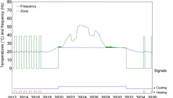
The top portion of Figure 7 shows the evolution of space and hot water temperatures as well as compressor frequency for a 24 h period starting at midnight at the beginning of the summer. The bottom part of the figure presents the corresponding control signals. All four operating modes are used alternatively during this period. Up to 𝑡 =3916.8 h, the space heating load is below the minimum capacity (2.6 kW) so the compressor runs at its minimum frequency (≈ 40 Hz) for the 𝐸𝑊𝑇 prevailing at that time. There is one instance of DHW production and the compressor runs at ≈ 60 Hz in that case. Then, for 𝑡 > 3916.8 h, the building gradually shifts from space heating to space cooling. The heat pump is off, except for a DHW production episode, and the space temperature increases up to 𝑡 = 3919.9 h when space cooling is required. Space cooling lasts until 𝑡 = 3931.5 h.
5100 512 514 516 518 520 522 524 526 5 10 15 20 25 30 0 20 40 60 80 Time (h) R oo m te m pe ra tu re ( °C ) C om pr es so r f re qu en cy (H z) Room temperature Room temperature Compressor frequency Compressor frequency
18 During that period there are 12 episodes of simultaneous space cooling and DHW production. The compressor frequency peaks at ≈ 80 Hz at 𝑡 = 3922.8 h when the space cooling load is maximum.
For 𝑡 > 3931.5 h, the cooling load decreases, the heat pump is off and the space temperature starts to fall up to 𝑡 = 3932.5 h, where the heat pump operates alternatively in space heating or in DHW production modes up to 𝑡 = 3936 h.
Throughout this 24 hour period, the space temperature remains within the set points and dead bands set in the controller for heating and cooling. At the beginning of the period, the space temperature fluctuates around the dead band due to the fact that the heating load is below the minimum capacity and the heat pump operates in on-off mode. At mid-day, during space cooling, there are small temperature fluctuations around 25°C caused by simultaneous cooling and DHW production modes. Finally, the water temperature at the top of the DHW tank remains stable at ≈50 °C throughout this period. Based on these results, it appears that the proposed model is able to handle all four modes of operation and to smoothly switch from one mode to the other.
Fig.7. Evolution of room space and hot water temperatures, compressor frequency and operating mode for a 24 h period.
19 The heat pump manufacturer specifies that hot water production modes are optional and it is possible to operate the heat pump in space conditioning modes only. Results of an annual simulation in this mode of operation is shown in Figure 8 for the same day that was presented in Figure 7. In this case, hot water is provided by the auxiliary electric heaters in the tank. The overall behavior is much the same as in Figure 7. However, the room temperature is slightly more stable than in Figure 7 at mid-day when space cooling is provided since the heat pump does not have to heat hot water. This seems to indicate that simultaneous space cooling and hot water production could result in room temperature fluctuations which could affect thermal comfort.
Fig. 8. Evolution of room temperature, frequency and operation mode for a 24h period, only space conditioning allowed.
5. Application
In this section, the variable capacity heat pump model is used in a comparative study against a regular fixed capacity heat pump. The fixed capacity heat pump has the same performance as the variable capacity heat pump at a fixed compressor frequency of 60 Hz. A 10 kW electric auxiliary heater is added for the case where the heat pump cannot meet
20 the building heating load. The energy consumption of the GHX pump was found to be relatively low at around 30 kWh per year and will not be included in the following energy consumption study.
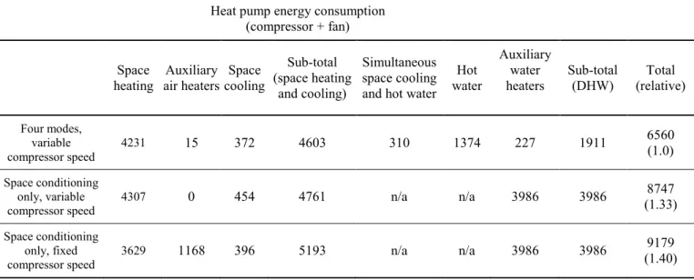
The resulting total energy consumption is shown in Table 4 for the following three cases: 1) Four modes, variable compressor speed. 2) Only space conditioning modes are allowed, variable compressor speed. 3) Only space conditioning modes are allowed, fixed compressor speed. The value of 𝑈𝐴 is set at 165 W/K based on the heat pump maximum capacity at 130 Hz.
Results show, as expected, that operating the heat pump with its full capabilities (four modes) leads to the lowest annual energy consumption (6560 kWh). When the heat pump operates at fixed speed, the total energy consumption is 40% higher (9179 kWh). In the intermediate case where the variable capacity heat pump does not provide hot water, the total energy consumption is 33% higher than in the four mode case. Most of the difference in the total annual energy consumption for the first two cases is due to DHW production. In the four mode case, the sum of the energy associated with DHW production either directly by the heat pump (1374 kWh) or by simultaneously providing space cooling (310 kWh) or with the auxiliary electric water heaters (227 kWh) is 52% lower than for the Table 4: Comparison of the annual energy consumption for three heat pump configurations, 𝑈𝐴 = 165 W/K (values in kWh) .
Heat pump energy consumption (compressor + fan)
Space
heating air heaters Auxiliary cooling Space
Sub-total (space heating
and cooling)
Simultaneous space cooling and hot water
Hot water
Auxiliary water
heaters Sub-total (DHW) (relative) Total
Four modes, variable compressor speed 4231 15 372 4603 310 1374 227 1911 6560 (1.0) Space conditioning only, variable
compressor speed 4307 0 454 4761 n/a n/a 3986 3986
8747 (1.33) Space conditioning
only, fixed
compressor speed 3629 1168 396 5193 n/a n/a 3986 3986
9179 (1.40)
21 second case (3986 kWh). In the third case, where the compressor speed is fixed at 60 Hz, the heat pump capacity is insufficient to meet the peak building loads and, in these cases, the auxiliary electric air heater is activated with corresponding annual energy consumption of 1193 kWh. As noted earlier, when the heat pump operates in simultaneous space cooling and DHW production, it requires 310 kWh on an annual basis. It should be noted that the space cooling load is not significant for this building in a heating dominated climate such as the one of Montreal. For warmer climates, it is expected that simultaneous space cooling and hot water production would occur more often thereby reducing the total energy consumption.
It is also possible to define a seasonal performance factor (SPF) as the ratio of the annual energy requirement for heating, cooling and DHW (=16650+3225+3986 kWh) over the annual total energy consumption. When the heat pump is working with the four modes of operation, the SPF is 3.64. In comparison, the SPF for the third case in Table 4 is 2.60. Another 𝑈𝐴 value for the building is used to perform annual energy calculations. In this case, the building peak load corresponds to the capacity of the heat pump at 60 Hz. The mid-range capacity of 5.3 kW is chosen to set the 𝑈𝐴 of the building to 106 W/K. However, it is not guaranteed that the fixed capacity heat pump provides exactly 5.3 kW if the compressor speed is fixed at 60 Hz as capacity depends largely on entering water temperature which varies throughout the year. Consequently, the heat pump capacity may be insufficient to meet the building load. For these cases, which only occur a few hours per year, the auxiliary electric air heater is activated.
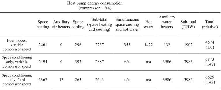
Table 5 presents the annual energy consumption for the same three configurations examined in Table 4 but for the new 𝑈𝐴 value. Much like the results presented in Table 4, the total annual energy consumption of the heat pump operating in all four modes is lower than for the variable capacity operating only in space conditioning modes. However, the difference here is larger at 47% because DHW production represents a larger part of the total annual energy consumption. It is interesting to note that the annual energy consumption of the fixed capacity heat pump (6629 kWh) is 3.5% lower than for the variable capacity heat pump which does not provide hot water (6873 kWh). This can be
22 caused by the fact that with this relatively low value of 𝑈𝐴, the variable capacity heat pump has to cycle on and off more frequently as it reaches the compressor frequency lower limits. As shown earlier, the heat pump COP is lower at the lower end of the frequency range. Finally, the SPF is 3.48 and 2.45 for the four modes of operation and the fixed capacity heat pump (third case), respectively.
6. Conclusion
This paper presents the development of a water-to-air variable capacity ground-source heat pump model. The model is designed to be used in TRNSYS and is based on the manufacturer’s steady-state performance maps. The heat pump modeled in this study can operate under four operating modes: space heating, dedicated space cooling, dedicated DHW production and simultaneous space cooling and DHW production. The heat pump is controlled by a PI-type thermostat which evaluates the required compressor frequency for the given condition.
The heat pump model is assembled around standard TRNSYS components. The action of the thermostat is modeled using a microprocessor logic controller (Type 40) along with PI controllers (Type 23). The performance maps are included in standard multi-dimensional Table 5 : Comparison of annual energy consumption for three heat pump configurations, 𝑈𝐴 = 106 W/K (values in kWh).
Heat pump energy consumption (compressor + fan)
Space
heating air heaters Auxiliary cooling Space
Sub-total (space heating
and cooling)
Simultaneous space cooling and hot water
Hot water
Auxiliary water
heaters Sub-total (DHW) (relative) Total
Four modes, variable compressor speed 2461 0 296 2757 353 1422 132 1907 4674 (1.0) Space conditioning only, variable
compressor speed 2494 0 393 2887 n/a n/a 3986 3986
6873 (1.47) Space conditioning
only, fixed
compressor speed 2367 13 263 2643 n/a n/a 3986 3986
6629 (1.42)
23 data interpolation tables (Type 581). These maps give the required frequency as a function of capacity. However, in reality, the compressor runs at the frequency determined by the controller and the capacity varies according to that frequency. To take this behavior into account, a relationship between capacity and frequency is determined (compressor frequency varies almost linearly with capacity), then the capacity corresponding to the frequency defined by the controller is used to read the performance data.
Results of one of the verification tests where the four modes of operation occur over a 24-hour period (Figure 7) show that the model is able to handle all four modes of operation and to smoothly switch from one mode to the other.
The proposed model is used in annual simulations of two residential buildings equipped with variable capacity and fixed capacity heat pumps. For the building with the highest heating and cooling loads, it is shown that the energy consumption of the fixed capacity heat pump is 40% higher than for the variable capacity heat pumps. The heat pump seasonal performance factor (SPF = ratio of the annual energy requirement for heating, cooling and DHW over the annual total energy consumption) operating with the four modes of operation is 3.64. The second case with the lower building loads was selected such that a fixed speed heat pump could handle the peak load and the annual heating requirement. In this case, the fixed speed heat pump uses slightly less energy for space heating as the variable speed heat pump is oversized and runs at the lower end of its frequency range where COP are lower. However, the SPF for the variable capacity heat pump operating with all four modes of operation remains relatively high at 3.48.
Acknowledgements
The financial support provided by the Natural Science and Engineering Research Council of Canada through a discovery grant and the Smart Net-Zero Energy Buildings Strategic Research Network is gratefully acknowledged.
24
References
Allard, Y., M. Kummert, M. Bernier, and A. Moreau. 2011. “Intermodel comparison and experimental validation of electrical water heater models in TRNSYS.” Proceedings of the 12th International IBPSA conference, Sydney, Australia, November 14-17.
Bagarella G., R. Lazzarin, and M. Noro. 2016. “Sizing strategy of on-off and modulating heat pump systems based on annual energy analysis.” International Journal of Refrigeration 65 : 183-193.
Baxter, V.D., C.K. Rice, R.W. Murphy, J. Munk, M. Ally, B. Shen, W.G. Craddick, and S.A. Hern. 2013. Ground Source Integrated Heat Pump (GS-IHP) Development. ORNL report. 40 pages.
Blervaque H., P. Stabat, S. Filfli, M. Schumann, and D. Marchio. 2016. “Variable-speed air-to-air heat pump modelling approaches for building energy simulation and comparison with experimental data.” Journal of building performance simulation 9 : 210-225.
Climate Master. 2014. Trilogy 45 Q-Mode (QE) Series. 52 pages.
Corberán J.M., 2016. “New trends and development in ground-source heat pumps.” In Advances in Ground-Source Heat Pump Systems, edited by S. Rees, 359-385. Woodhead Publishing Series.
Corberán J.M., D. Donadello, I. Martínez-Galván, and C. Montagud. 2013. “Partialization losses of ON/OFF operation of water-to-water refrigeration/heat pump units.” International Journal of refrigeration 36 : 2251-2261.
Del Col, D., G. Benassi, M. Mantovan, and M. Azzolin. 2012. “Energy efficiency in a ground source heat pump with variable speed drives.” International Refrigeration and Air Conditioning Conference. Paper #1342.
Eslami-nejad, P., and M. Bernier. 2009. “Impact of grey water heat recovery on the electrical demand of domestic hot water heaters.” Proceedings of the 11th International
IBPSA conference, Glasgow, Scotland, July 27-30.
Karlsson F., and P. Fahlén. 2007a. “Capacity-controlled ground source heat pumps in hydronic heating systems.” International Journal of Refrigeration 30 : 221-229.
Karlsson F., and P. Fahlén. 2007b. “Impact of design and thermal inertia on the energy saving potential of capacity controlled heat pump heating systems.” International Journal of Refrigeration 31 : 1094-1103.
Klein, S.A, et al. 2014. TRNSYS 17 – a transient system simulation program, Solar Energy Laboratory, University of Wisconsin-Madison.
25 Liu, X. 2014. “Advance Ground Source Heat Pump Technology for Very Low Energy Buildings.” https://cercbee.lbl.gov/sites/all/files/attachments/Day%201-Panel%203-GSHP-ORNL-Xiaobing.FINAL_.pdf.
Madani H., N. Ahmadi, J. Claesson, and P. Lundqvist. 2010. “Experimental analysis of a variable capacity heat pump system focusing on the compressor an inverter loss behavior.” International refrigeration and air conditioning conference. Paper #1063.
Madani H., J. Claesson, and P. Lundqvist. 2011. “Capacity control in ground source heat pump systems part II: Comparative analysis between on/off controlled and variable capacity systems.” International Journal of Refrigeration 34 : 934-1942.
Ndiaye D., and M. Bernier. 2012. “Transient model of a geothermal heat pump in cycling conditions – Part A: The model.” International Journal of Refrigeration 35 : 2110-2123. Ndiaye D., and M. Bernier, M. 2012. “Transient model of a geothermal heat pump in cycling conditions – Part B: Experimental validation and results.” International Journal of Refrigeration 35 : 2124-2137.
Nyika S., W.T. Horton, S.O. Holloway, and J.E. Braun. 2014. “Generalized performance maps for variable-speed, ducted, residential heat pumps.” ASHRAE Transactions 120(2). Rice, K., V. Baxter S. Hern, T. McDowell, J. Munk, and B. Shen. 2013. “Development of a residential Ground-Source Integrated Heat Pump.” Paper presented at the annual winter meeting of ASHRAE, Dallas, Texas.
Simon F., J. Ordoñez, T.A. Reddy, A. Girard, and T. Muneer. 2016. “Developing multiple regression models from the manufacturer’s ground-source heat pump catalogue data.” Renewable Energy 95 : 413-421.
TESS. 2012. TESS Component Libraries. Madison, Wisconsin: Thermal Energy Systems Specialists.
Waddicor D., E. Fuentes, M. Azar, and J. Salom. 2016. “Partial load efficiency degradation of a water-to-water heat pump under fixed set-point control.” Applied Thermal Engineering 106 : 275-285.
Zhao L., L.L. Zhao, Q. Zhang, and G.L. Ding. 2003. “Theoretical and basic experimental analysis on load adjustment of geothermal heat pump systems.” Energy Conversion and Management 44 : 1-9.