HAL Id: hal-00329156
https://hal.archives-ouvertes.fr/hal-00329156
Submitted on 1 Jan 2001
HAL is a multi-disciplinary open access
archive for the deposit and dissemination of
sci-entific research documents, whether they are
pub-lished or not. The documents may come from
teaching and research institutions in France or
abroad, or from public or private research centers.
L’archive ouverte pluridisciplinaire HAL, est
destinée au dépôt et à la diffusion de documents
scientifiques de niveau recherche, publiés ou non,
émanant des établissements d’enseignement et de
recherche français ou étrangers, des laboratoires
publics ou privés.
Letter to the EditorEffects of hot oxygen in the
ionosphere: TRANSCAR simulations
D. Alcaydé, P.-L. Blelly, W. Kofman, A. Litvin, W. L. Oliver
To cite this version:
D. Alcaydé, P.-L. Blelly, W. Kofman, A. Litvin, W. L. Oliver. Letter to the EditorEffects of hot
oxygen in the ionosphere: TRANSCAR simulations. Annales Geophysicae, European Geosciences
Union, 2001, 19 (2), pp.257-261. �hal-00329156�
Annales
Geophysicae
Letter to the Editor
Effects of hot oxygen in the ionosphere:
TRANSCAR simulations
D. Alcayd´e1, P.-L. Blelly1, W. Kofman2, A. Litvin3, and W. L. Oliver3
1CESR, CNRS, Toulouse, France 2LPG, CNRS, Grenoble, France
3Boston University, Massachusetts, USA
Received: 7 November 2000 – Revised: 18 December 2000 – Accepted: 20 December 2000
Abstract. Recent studies of the ion energy balance in the
mid-latitude ionosphere have led to the suggestion that hot neutral atomic oxygen may play a significant role; the pres-ence of a population of hot O could explain some of the prob-lems met in balancing the ion energy budget for Incoherent Scatter (IS) observations. The aim of the present study is to look at such effects by using numerical simulation. The TRANSCAR model is a time-dependent, 13-moment iono-sphere model developed for high latitude studies. It was first adapted for mid-latitude conditions. In a first step the model was calibrated and cross-checked with St. Santin IS measure-ments for the winter case of 27 January 1972 around noon us-ing, in particular, the MSIS neutral atmosphere model. This provides a reference diurnal variation of the ionosphere. The second step investigated the influence of a maxwellian pop-ulation of hot neutral atomic oxygen introduced in addition to the standard neutral atmosphere. The paper describes the initial comparison between the model and St. Santin IS data, and then the effects induced by a hot atomic oxygen popula-tion.
Key words. Ionosphere (ionosphere-atmosphere
interac-tions; ion chemistry and composition; mid-latitude iono-sphere)
1 Introduction
There is more and more evidence that a hot part of the oxy-gen velocity distribution exists and plays an important role in thermosphere-ionosphere interactions. The first evidence was the discrepancy between the oxygen density inferred from incoherent scatter data and that measured by OGO 6: Hedin and Alcayd´e (1974) showed individual conjunction agreements for daytime measurements, but significant dis-crepancies between OGO 6 and St. Santin diurnal variations, in particular, around sunrise and sunset. Another indica-tion was suggested after studies of the collision frequency Correspondence to: D. Alcayd´e ([email protected])
νO+−O between ion O+ and the neutral atomic oxygen O, using either the energy balance or momentum balance equa-tion (Oliver and Glotfelty, 1996). These two methods lead to as much as 60% different solutions for the collision fre-quencies. Oliver (1997) showed that the inclusion of a small fraction of hot oxygen can bring the results of these two methods into agreement. Despite the lack of direct measure-ments of the hot O component in the upper thermosphere, strong indications of a high-energy non-maxwellian tail with equivalent temperatures ranging from 4000 to 6000 K have been inferred from airglow measurements (Yee et al., 1980; Cotton et al., 1993). A recent study of the 630nm airglow emission (Shematovich et al., 1999) led to the conclusion that hot O(1D) emissions have to be taken into account for accurate neutral temperature measurements in the thermo-sphere. Oliver and Schoendorf (1999) inferred hot oxygen variations from incoherent scatter data, and Schoendorf et al. (2000) used a simple method of deriving hot O profiles from its mass and energy conservation equations. These previous studies motivated the current work to quantitatively model the effect of the hot oxygen component on the ionosphere. These simulations have been made using the TRANSCAR ionosphere model (Blelly et al., 1996). The effects of an additional small fraction of hot O, added to the MSIS atmo-sphere model (Hedin, 1987, 1991) on the ion energy balance, is self-consistently modelled. Finally, the resulting effects are shown on the method used to determine the exospheric temperature and the oxygen density from the incoherent scat-ter data.
2 Method of n[O] and exospheric temperature determination
The ion energy balance equation for an altitude profile is solved in order to determine the neutral parameters. These parameters are the oxygen density as a function of altitude and the exospheric temperature, which, with the assumption of a Bates profile shape, gives the complete description of the
258 D. Alcayd´e et al.: Ionosphere and hot O: TRANSCAR simulations thermosphere. The ion energy equation taken in the steady
state is
Lei = Lin (1)
where Lei represents the heat given by the electrons to the
ions and Lin the losses of energy from the ions to the
neu-trals. This equation can admit a simplified form for altitudes where the only ion is O+and the main neutral component is atomic oxygen (above 280 km for mid-latitudes)
Lin =
3
2nik (Ti − Tn) νO+−O, (2)
Lei = 3 nek (Te − Ti) νei, (3)
where ne, ni are the ion and electron densities (charge
neu-trality implies ne=ni), Teand Ti the electron and ion
tem-peratures and Tn the neutral temperature; νO+−O is the res-onant energy-dependent collision frequency, νei is the
clas-sical electron-ion coulomb collision frequency, and k is the Boltzman constant. Substituting Eq. 2 and 3 in Eq. 1 leads to
νO+−O(Ti −Tn) = 2 νei(Te − Ti) (4)
with, following Banks (1966),
νO+−O ∝ n[O]
p
Ti +Tn, and νei ∝ neTe−1.5. (5)
From Eq. 4–5, one can express Tias a function Ti∗which
de-pends on the altitude profiles of the neutral temperature and atomic oxygen concentration n[O], and on measured iono-spheric parameters, Te, Tiand ne
Ti∗ = Tn +κ Te 1 + κ , with κ ∝ Te−1.5ne √ Ti +Tnn[O] . (6)
If one assumes that in the upper atmosphere (above 300 km altitude), the neutral temperature has reached its asymptotic exospheric value T∞and furthermore, that the thermal atomic
oxygen is in diffusive equilibrium, then T∗
i can be fitted to Ti
using two free parameters, namely the exospheric tempera-ture T∞and the atomic oxygen concentration at a reference
altitude (Bauer et al., 1970; Alcayd´e and Bauer, 1977).
3 TRANSCAR use to check the method
TRANSCAR modelling can introduce in a complete way the complex interactions between the ionosphere and neutral at-mosphere. TRANSCAR uses the 13-moment approximation of ionosphere transport (see Blelly and Schunk (1993) for a complete description of the set of equations, and Blelly et al. (1996) for a description of the model). The ion energy equation can be written as a general time-dependent equilib-rium of energy exchanges resulting from electron-ion colli-sion Lei, ion-neutrals collisions Lin, friction between ions
and neutrals and transport effects
nik ∂ Ti ∂ t = Lei −Lin +LFrict + LTransp. (7) 500 1000 1500 2000 2500 3000 3500 200 250 300 350 400 450
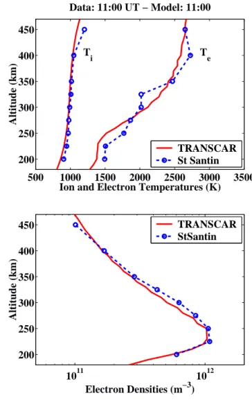
Ion and Electron Temperatures (K)
Altitude (km) Data: 11:00 UT − Model: 11:00 T i Te TRANSCAR St Santin 1011 1012 200 250 300 350 400 450 Electron Densities (m−3) Altitude (km) TRANSCAR StSantin
Fig. 1. Altitude profile of electron densities (bottom panel),
elec-tron and ion temperatures (top panel) observed by the St. Santin Incoherent Scatter on 27 January 1972 (symbols and broken lines), and TRANSCAR simulation results.
TRANSCAR assumes as external inputs (for mid-latitude con-ditions) a solar EUV flux indexed to the 10.7 cm radio flux in-dex, the neutral atmosphere model provided by MSIS (Hedin, 1987, 1991), and the neutral wind model provided by HWM (Hedin et al., 1991) for ion-neutral frictional effects. Chem-ical equilibrium is assumed in the lower boundary (90 km), while at the upper boundary a downward electron heat flux is injected for adjusting observed electron temperature profiles. All other ion and electron parameters (concentrations, field-aligned velocities, temperature and heat flow) are solved vs. time and altitude. Figure 1 shows the model results for the Solar, Local Time and Seasonal conditions that were ob-served by the St. Santin Incoherent Scatter facility obser-vations of 27 January 1972 (11:00 UT). The only purpose of this comparison is to show that TRANSCAR can ade-quately model the mid-latitude ionosphere observed above St. Santin, and the good agreement between data and model in Fig. 1 gives confidence to the model results. Now, given
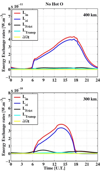
0 3 6 9 12 15 18 21 24 −1 0 1 2 3 4 5 6 7 8x 10 −11
Energy Exchange rates [W.m
−3 ] No Hot O 400 km L in L ei L Frict L Transp ∂/∂t 0 3 6 9 12 15 18 21 24 −1 0 1 2 3 4 5 6 7 8x 10 −10 Time [U.T.]
Energy Exchange rates [W.m
−3 ] Lin 300 km L ei L Frict L Transp ∂/∂t
Fig. 2. Energy equation terms (see text and Eq. 7) extracted from
the TRANSCAR outputs at 400 km (top panel) and 300 km (bottom panel) altitudes.
diurnal TRANSCAR results, one can evaluate the various terms entering Eq. 7, in order to a-posteriori test the method of deducing neutral parameters by fitting with Eq. 6. Figure 2 shows the time variation of the various terms of Eq. 7, ex-tracted from TRANSCAR results at 300 and 400 km. This fig-ure shows that the Lei =Linapproximation can be
consid-ered good but not perfect. Diurnal discrepancies between the two terms appear to be essentially due to neutral wind (fric-tional) effects and not surprisingly, are more sensitive at 300 km than at 400 km. But the discrepancy appears to be 10%, at most. With TRANSCAR profiles one is then able to use the fitting procedure of Eq. 6 in order to check the resulting esti-mates of the exospheric temperature and n[O] concentration (results are shown in Fig. 3). Error bars are calculated by placing an estimated error on the model Ti profile of 1% (i.e.
10 K for a 1000 K ion temperature). The resulting errors on the exospheric temperature are approximately 15 K. Figure 3 shows that most of the T∞diurnal variation inferred from the
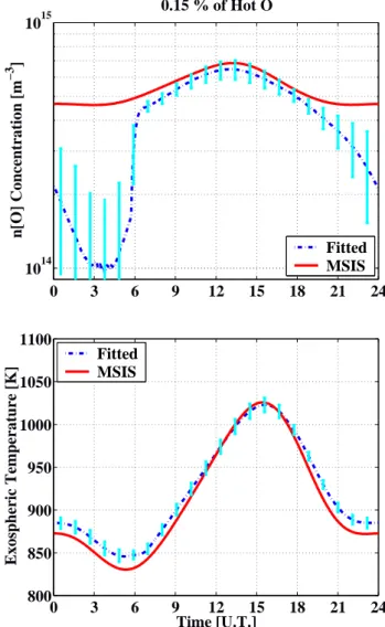
0 3 6 9 12 15 18 21 24 1014 1015 n[O] Concentration [m −3 ] No Hot O Fitted MSIS 0 3 6 9 12 15 18 21 24 800 850 900 950 1000 1050 1100 Time [U.T.] Exospheric Temperature [K] Fitted MSIS
Fig. 3. Altitude profiles of ne, Teand Tigiven by TRANSCAR
out-puts were fitted to infer the exospheric temperature (bottom panel) and the atomic oxygen concentration at 300 km altitude (top panel). The MSIS model temperatures and concentrations that were used in the TRANSCAR model are shown for comparison. Case with no additional hot oxygen population.
fits agrees quite well with the MSIS model which was used in the simulations. The same holds also for the inferred n[O] densities, with estimated errors of 10%, which correctly take into account the model-fitted density discrepancies. This is true during most of the daytime while at night and around dusk and dawn, the energy balance of Eq. 4–5 is ensured by the trivial equation Te = Ti = Tn. These dusk, night and
dawn periods had therefore to be considered as safe for T∞
determination but not reliable for n[O]. The next step is now to introduce an extra population of hot oxygen in the TRAN-SCAR simulations and to check its effects upon the previous results. This will be done by using these new TRANSCAR results and applying the n[O] and T∞fit, but ignoring the
260 D. Alcayd´e et al.: Ionosphere and hot O: TRANSCAR simulations 0 3 6 9 12 15 18 21 24 −1 0 1 2 3 4 5 6 7 8x 10 −11
Energy Exchange rates [W.m
−3 ] 0.15 % of Hot O 400 km L in L ei L Frict L Transp ∂/∂t L Hot O 0 3 6 9 12 15 18 21 24 −1 0 1 2 3 4 5 6 7 8x 10 −10 Time [U.T.]
Energy Exchange rates [W.m
−3 ] Lin 300 km L ei L Frict L Transp ∂/∂t L Hot O
Fig. 4. Same as Fig. 2, but a population of hot O has been added to
the standard MSIS neutral atmosphere: Hot O concentration is kept constant vs. time such that at noon {n[OHot]/n[O]}400km=0.15%; its altitude profile is defined with an equivalent exospheric temper-ature of 4000 K.
4 Introducing a hot oxygen population
As the rate of ion heat exchange depends on temperature dif-ferences (Eq. 4), even a small fraction of hot oxygen O∗can imply significant energy exchanges. Assuming an extra pop-ulation of suprathermal oxygen with a maxwellian distribu-tion with characteristic temperature TO∗, Eq. 4 should be re-written
νO+−O(Ti −Tn) = 2 νei(Te − Ti)
+νO+−O∗(TO∗−Ti) (8)
with, similarly to Eq. 5,
νO+−O∗ ∝ n[O∗]
p
Ti +TO∗. (9)
In the case where the O∗component has a temperature higher than the ion temperature, the last term in Eq. 8 turns to be
0 3 6 9 12 15 18 21 24 1014 1015 n[O] Concentration [m −3 ] 0.15 % of Hot O Fitted MSIS 0 3 6 9 12 15 18 21 24 800 850 900 950 1000 1050 1100 Time [U.T.] Exospheric Temperature [K] Fitted MSIS
Fig. 5. Same as Fig. 3, but a population of hot O has been added to
the standard MSIS neutral atmosphere: Hot O concentration is kept constant vs. time such that at noon {n[OHot]/n[O]}400km=0.15%; its altitude profile is defined with an equivalent exospheric temper-ature of 4000 K. However, n[O] and T∞fits are done ignoring the
presence of this minor neutral constituent.
positive and acts as a net heat source for the ions. Hence, neglecting this source term requires that the sink term be re-duced accordingly by underestimating n[O] to balance the ion heat inflow and outflow. Again TRANSCAR was used to quantitatively study this effect. In a first step, a popula-tion of hot oxygen was added to the standard neutral atmo-sphere model in the following way. As the purpose is only to demonstrate the effects of a small fraction of hot O in the thermosphere, only a simple altitude profile of hot oxygen was used, and that profile was kept constant throughout the day. Hot O was assumed to be in diffusive equilibrium with a scale height appropriate to a temperature of 4000K, and its density at 400 km altitude was set to be between 0.15% and 0.5% of the thermal O density at noon. This fractional hot O population is taken into account in TRANSCAR by its
collisional effects (Eq. 9) in the momentum, energy and heat flux equations. Figure 4 is similar to Fig. 2 with now the additional term LHotO computed from the new TRANSCAR results with 0.15% hot O at 400 km at noon. The presence of the small fraction of hot O at 300 and 400 km implies a significant increase of the electron-ion Lei and ion-neutral
Lin energy exchanges. Note that Lei increases because hot
O heats the electrons as well the ions. While LHotO appears to be negligible around noon at 300 km altitude, its influence increases with increasing altitude because of the large hot O scale height, and becomes greatest near and after sunset. Sources from hot neutrals play a large role and are compa-rable to sources from thermal neutrals at night. If one tests again the atomic oxygen fitting method applied on these new TRANSCAR results, but ignores in the fitting procedure the presence of the hot O population, then one obtains the results displayed in Fig. 5. This figure shows that the resulting ex-ospheric temperatures are still in reasonable agreement with the initial model, but with systematic errors of about 20 K, i.e. larger than the inferred statistical errors. However, the inferred atomic oxygen concentrations present, as expected, important disagreements, especially well before sunset and after sunrise, and throughout the night. Increasing the frac-tion of hot O obviously makes the situafrac-tion worse. These results confirm that, as suggested by Oliver (1997), neglect-ing the presence of the hot O may be a major drawback in the incoherent scatter data fitting.
5 Discussion and conclusion
The simulations with TRANSCAR show that even a small fraction of hot O has a significant impact on the ion en-ergy balance, and affects O determination greatly at certain times of day while the exospheric temperature determination is only modestly affected. Particular deviations are found near sunset/sunrise periods for the densities, even with small fractions of hot O. As suggested by Oliver (1997), if one as-sumes that MSIS model’s cold O values are reliable and the heat balance analysis with the hot O terms are included, this becomes a candidate method to infer hot O concentration in-stead of cold O but the sensitivity of the method to neglected terms and assumptions needs to be checked carefully. In par-ticular, our study shows frictional effects to be of a similar order of magnitude as hot O effects. Also, the shape of the hot O profile is largely unknown and the assumptions made for that shape may affect the hot O density deduction sub-stantially. Finally, whether one can separate the dusk-night-dawn uncertainties on n[O] determination from hot O effects is certainly challenging. These investigation can be aided by the use of TRANSCAR as a quantitative tool and will be the subject of future studies.
Acknowledgement. The St. Santin Incoherent Scatter facility was
supported by the CNET and operated with a financial support from the CNRS.
Topical Editor Mark Lester thanks J. E. Salah for his help in evaluating this paper.
References
Alcayd´e, D. and Bauer, P., Mod´elisation des concentrations d’oxyg`ene atomique observ´ees par diffusion incoh´erente, An-nales de G´eophysique, 33, 305–320, 1977.
Banks, P. M., Collision frequencies and energy transfer: Ions, Planet. Space Sci, 14, 1105–1122, 1966.
Bauer, P., Waldteufel, Ph., and Alcayd´e, D., Diurnal variations of the atomic oxygen density and temperature determined from in-coherent scatter measurements in the ionospheric F region, J. Geophys. Res., 75, 4825–4832, 1970.
Blelly, P.-L. and Schunk, R. W., A comparative study between stan-dard, 8-, 13- and 16-moment approximations, Ann. Geophys., 11, 443–469, 1993.
Blelly, P.-L., Robineau, A., Lilensten, J., and Lummerzheim, D., 8-moment fluid models of the terrestrial high latitude ionosphere between 100 and 3000 km, in Solar Terrestrial Energy Program (STEP): Handbook of Ionospheric Models, R. W. Schunk, ed., 53–72, 1996.
Cotton, D. M., Gladstone, G. R., and Chakrabarti, S., Sounding rocket observation of a hot oxygen geocorona, J. Geophys. Res., 98, 21651–21657, 1993.
Hedin, A. E., MSIS-86 thermospheric model, J. Geophys. Res., 92, 4649–4662, 1987.
Hedin, A. E., Extension of the MSIS thermosphere model into the middle and lower atmosphere, J. Geophys. Res., 96, 1159–1172, 1991.
Hedin, A. E. and Alcayd´e, D., Comparison of atomic oxygen mea-surements by incoherent scatter and satellite born mass spec-trometer technique, J. Geophys. Res., 79, 1579–1581, 1974. Hedin, A. E., Spencer, N. W., Biondi, M. A., Burnside, R. G.,
Her-nandez, G., and Johnson, R. M., Revised global model of ther-mosphere winds using satellite and ground-based observations, J. Geophys. Res., 96, 7657–7688, 1991.
Oliver, W. L., Hot O and the ion energy budget, J. Geophys. Res., 102, 2503–2511, 1997.
Oliver, W. L. and Glotfelty, K., O+−O collision cross section and long term F-region O density variations deduced from the iono-spheric energy budget, J. Geophys. Res., 101, 21769–21784, 1996.
Oliver, W. L. and Schoendorf, J., Variations of hot O in the thermo-sphere, Geophys. Res. Lett., 26, 2829–2832, 1999.
Schoendorf, J., Young, L. A., and Oliver, W. L., Hot oxygen pro-files for incoherent scatter radar analysis of ion energy balance, J. Geophys. Res., 105, 12823–12832, 2000.
Shematovich, V., G´erard, J. C., Bisikalo, V., and Hubert, B., Ther-malisation of O(1D) atoms in the thermosphere, J. Geophys. Res, 104, 4287–4293, 1999.
Yee, J. H., Meriwether Jr., J. W., and Hays, P. B., Detection of a corona of fast oxygen atoms during solar maximum, J. Geophys. Res., 85, 3396–3400, 1980.