2017 — Predictive numerical modeling of the behavior of rockfill dams

(1)

Predictive Numerical Modeling of the Behavior of

Rockfill Dams

by

Ardalan AKBARI HAMED

THESIS PRESENTED TO ÉCOLE DE TECHNOLOGIE SUPÉRIEURE

IN PARTIAL FULFILLMENT FOR A MASTER’S DEGREE

WITH THESIS IN PERSONAL CONCENTRATION

M. A. S

c

.

MONTREAL, 13TH_{FEBRUARY 2017}

ÉCOLE DE TECHNOLOGIE SUPÉRIEURE UNIVERSITÉ DU QUÉBEC

(2)

This Creative Commons licence allows readers to download this work and share it with others as long as the author is credited. The content of this work can’t be modified in any way or used commercially.

(3)

BOARD OF EXAMINERS THESIS M.SC.A.

THIS THESIS HAS BEEN EVALUATED BY THE FOLLOWING BOARD OF EXAMINERS

Mr. Azzeddine. Sulaïmani, Eng., Ph.D., Thesis Supervisor

Professor, Department of Mechanical Engineering at École de technologie supérieure

Mr. Daniel Verret, Eng., M.Sc., Industrial Thesis Co-supervisor Hydro-Québec, Production Division

Mr. Tan Pham, Eng., Ph.D., President of the Board of Examiners

Professor, Department of Mechanical Engineering at École de technologie supérieure

Mr. Jean-Marie Konrad, Eng., Ph.D., External Evaluator

Professor, Department of Civil Engineering and Water Engineering at Laval University

THIS THESIS WAS PRENSENTED AND DEFENDED

IN THE PRESENCE OF A BOARD OF EXAMINERS AND PUBLIC 6TH_{FEBRUARY 2017}

(4)

(5)

ACKNOWLEDGMENT

This work is a part of the Industrial Innovation Scholarships Program supported by Hydro-Québec, NSERC (Natural Sciences and Engineering Research Council of Canada), and FRQNT (Fond de recherché du Québec -Nature et Technologies).

I would like to sincerely thank my supervisor, Professor Azzeddine Soulaïmani, for his confidence in me, advice, and support. I would also like to express my deepest gratitude to my co-supervisor, Eng. Daniel Verret for his guidance, encouragements, and invaluable helps throughout this study. My sincere appreciation is extended to Eng Eric Péloquin and Eng Annick Bigras.

Finally, with all my heart, I would like to thank my parents for their supports and encouragements.

(6)

(7)

MODÉLISATION NUMÉRIQUE PRÉDICTIVE DU COMPORTEMENT DE BARRAGES EN ENROCHEMENTS

Ardalan AKBARI HAMED

RÉSUMÉ

Le choix approprié d'un modèle constitutif du sol est l'une des parties les plus importantes lors des analyses numériques par éléments finis ou différences finies. En effet, il existe plusieurs modèles constitutifs du sol, mais aucun d'entre eux ne peut reproduire tous les aspects du comportement réel du sol. Dans cette recherche, différents modèles constitutifs du sol ont été étudiés à l'aide d'un test triaxial et œdométrique. Deux logiciels pour éléments finis, Plaxis et ZSoil, ont été utilisés pour la simulation numérique. Les résultats des simulations numériques et les résultats expérimentaux ont été comparés les uns aux autres. Des comparaisons ont été effectuées pour observer lequel de ces modèles obtient des résultats plus proches des données expérimentales.

Dans la seconde partie de cette étude, on s’intéresse à la modélisation du barrage X. Le barrage X est un barrage d'enrochement en asphalte construit sur une rivière du Québec, dans la région de la Côte-Nord, au Québec. Le problème a été analysé numériquement en utilisant le logiciel des éléments finis pour différentes étapes de construction et après la mise en eau. Les données mesurées à partir de la surveillance et l'analyse numérique illustrent une réponse appropriée du barrage X. Le but de cette recherche est d'étudier numériquement la performance des solutions numériques en considérant différents modèles constitutifs du sol, tels que Duncan-Chang (1970), Mohr-Coulomb et le modèle Hardening soil (H.S.). Des comparaisons ont été effectuées pour observer lequel de ces modèles obtient des résultats plus proches de ces mesures.

Mots-clés: barrage d'enrochement, éléments finis, modèle constitutif du sol, analyse numérique

(8)

(9)

PREDICTIVE NUMERICAL MODELING OF THE BEHAVIOR OF ROCKFILL DAMS

Ardalan AKBARI HAMED ABSTRACT

Choosing an appropriate soil constitutive model is one of the most important elements of a successful finite element or finite difference analysis of soil behavior. There are several soil constitutive models; however, none of them can reproduce all aspects of real soil behavior. In this research, various constitutive soil models have been studied through triaxial and oedometer tests. Two finite element software applications, namely, Plaxis and Zsoil, were used for numerical analysis. Subsequently, the numerical simulation values were compared with experimental test results to determine which of these constitutive soil models obtained the closest results to the experimental data.

The main focus of the study is the comparison between the measured data from monitoring instruments and the numerical analysis results of the Dam-X. Dam-X is an asphaltic core rockfill dam constructed on a River in the North Shore region of Québec. The rockfill dam behavior was analyzed numerically using finite element programs for different stages of construction and after impoundment. The measured data from monitoring and numerical analysis results represent the appropriate response of the Dam-X. The aim of this study is to evaluate the performance of numerical solutions by considering various constitutive soil models, namely, the Duncan–Chang, MC, and HS models. Comparisons were conducted to determine which of these constitutive soil models obtained the closest results to the measurements.

(10)

(11)

TABLE OF CONTENTS

Page

INTRODUCTION ...1

CHAPTER 1 A REVIEW OF CONSTITUTIVE SOIL MODELS ...3

1.1 Introduction ...3

1.2 Constitutive soil model ...3

1.2.1 Hyperbolic model... 5

1.2.2 Hardening soil model ... 13

1.2.3 Hardening soil-small strain model ... 21

CHAPTER 2 COMPARISON AMONG DIFFERENT CONSTITUTIVE SOIL MODELS THROUGH TRIAXIAL AND OEDOMETER TESTS ...23

2.2 Triaxial test ...23

2.3 Finite element modeling ...24

2.3.1 Geometry of model and boundary conditions in Plaxis ... 24

2.3.2 Geometry of model and boundary condition in Zsoil ... 26

2.4 Experimental data ...27

2.5 Application of constitutive soil models ...29

2.5.1 Mohr–Coulomb model ... 29

2.5.3 Hardening small strain soil model ... 38

2.5.4 Duncan–Chang soil model ... 41

2.6 Comparison between constitutive soil models ...45

2.7 Oedometer test ...50

2.8.1 Geometry of model and boundary conditions in Plaxis ... 51

2.8.2 Model geometry and boundary conditions in Zsoil ... 52

2.9 Experimental data ...53

2.10 Application of constitutive soil models ...55

2.10.1 Duncan–Chang Model ... 55

2.10.3 Hardening small strain constitutive soil model ... 59

2.11 Comparison between constitutive soil models ...61

2.12 Updated mesh results for triaxial test...64

CHAPTER 3 NUMERICAL SIMULATIONS FOR DAM-X ...73

3.2 Asphalt core dam ...73

3.3 Dam-X...74

3.4 Typical cross section ...75

(12)

3.6 Instrumentation ...80

3.8 Displacement contours at the end of construction ...84

3.9 Comparison between measured data and numerical simulations after construction ...88

3.9.1 Comparison between measured and computed displacements after construction (inclinometer INV-01) ... 88

3.9.2 Comparison between measured and computed displacements after construction ( inclinometer INV-02) ... 90

3.9.3 Comparison between measured and computed displacements after construction ( inclinometer INV-03) ... 92

3.9.4 Comparison between measured and computed displacements after construction (INH-01 and INH-02) ... 94

3.10 Comparison between Plaxis and Zsoil ...97

3.11 Numerical simulation procedure for wetting ...101

3.11.1 Justo approach ... 102

3.11.2 Nobari–Duncan approach ... 102

3.11.3 Escuder Procedure ... 105

3.11.4 Plaxis Procedure ... 109

3.12 Results after impoundment ...110

3.12.1 Comparison between measured and computed displacements after impoundment (inclinometer INV-01) ... 113

3.12.4 Comparison between measured and computed displacements after impoundment (inclinometer INH-01) ... 120

3.13 Shear wave velocity measurement ...121

3.13.1 Material properties for zone 3O and 3P ... 121

3.13.2 Comparison between measured and computed displacements ... 127

3.14 Concluding remarks ...132 CONCLUSION………..135 RECOMMENDATIONS ...137 APPENDIX I……….139 APPENDIX II………165 BIBLIOGRAPHY ………..177

(13)

LIST OF TABLES

Page Table 1.1 Summary of Hyperbolic parameters (Wong et Duncan, 1974) ...8 Table 1.2 Summary of Hyperbolic parameters

(Duncan, Wong et Mabry, 1980) ...11 Table 2.1 Mesh size influences on deviatoric stress for the Hardening

soil model in Plaxis software ...26 Table 2.2 Mesh size influences on deviatoric stress for the Hardening

soil model in Zsoil software ...27 Table 2.3 Soil properties used in the MC model for loose sand ...30 Table 2.4 Soil properties used in the MC model for dense sand ...31 Table 2.5 Soil properties used in the HS model for dense and

loose sand (Brinkgreve, 2007) ...34 Table 2.6 Supplemental HS Small soil parameters for loose and

dense Hostun sand (Brinkgreve, 2007) ...38 Table 2.7 Soil properties used in the model for dense and loose sand ...42 Table 3.1 Hardening soil model parameters used for rockfill dam simulation ...78 Table 3.2 Mohr-Coulomb soil model parameters used for

rockfill dam simulation ...79 Table 3.3 Duncan-Chang soil model parameters used for

rockfill dam simulation ...79 Table 3.4 Mesh size influences on total displacement in Plaxis software ...82 Table 3.5 Absolute maximum horizontal and vertical displacement

resulted by FE analysis at section INV-1 ...90 Table 3.6 Absolute maximum horizontal and vertical displacement

(14)

Table 3.8 Absolute maximum vertical displacement resulted by FE

analysis at section INH-1 ...95 Table 3.9 Absolute maximum vertical displacement resulted by FE

analysis at section INH-2 ...96 Table 3.10 Associated bounds (Simon Grenier, 2010) ...107 Table 3.11 Absolute maximum horizontal and vertical displacement

resulted by FE analysis at section INV-3 ...119 Table 3.14 Absolute maximum vertical displacement resulted by FE

analysis at section INH-1 ...121 Table 3.15 Mohr-Coulomb soil model parameters used for rockfill dam

simulation at zone 3O ...124 Table 3.16 Mohr-Coulomb soil model parameters used for rockfill dam

simulation at zone 3P ...124 Table 3.17 HS soil model parameters used for rockfill dam simulation

at zone 3O ...125 Table 3.18 HS soil model parameters used for rockfill dam simulation

at zone 3P ...125 Table 3.19 HSS soil model parameters used for rockfill dam simulation

at zone 3O ...126 Table 3.20 HSS soil model parameters used for rockfill dam simulation

(15)

LIST OF FIGURES

Page Figure 1.1 Comparison of typical stress and strain curve with hyperbola

(Al-Shayea et al., 2001) ...5

Figure 1.2 Transformed Hyperbolic stress- strain curve (Duncan et Chang, 1970) ...6

Figure 1.3 Mohr envelope for Oroville dam core material (Wong et Duncan, 1974) ...9

Figure 1.4 Hyperbolic axial strain – radial strain curve (Wong et Duncan, 1974) ...10

Figure 1.5 Variation of bulk modulus with confining pressure (Duncan, Wong et Mabry, 1980) ...12

Figure 1.6 Hyperbolic stress-strain relationship for a standard drained triaxial test in primary loading (Brinkgreve et Broere, 2006) ...14

Figure 1.7 Explanation of in the oedometer test (Brinkgreve et Broere, 2006) ...16

Figure 1.8 Dilatancy cut-off (Brinkgreve et Broere, 2006) ...19

Figure 1.9 Yield surface of the hardening soil model in p-q plane (Brinkgreve et Broere, 2006) ...20

Figure 1.10 The yield contour of the hardening soil model in stress space (Brinkgreve et Broere, 2006) ...20

Figure 1.11 Schematic presentation of the HS model, stiffness-strain behavior (Obrzud, 2010) ...22

Figure 2.1 Triaxial loading condition (Surarak et al., 2012) ...24

Figure 2.2 Plot of the mesh in Plaxis ...25

Figure 2.3 Plot of the mesh in Zsoil ...27

Figure 2.4 Results of drained triaxial test on loose Hostun sand (Brinkgreve, 2007)...28

Figure 2.5 Results of drained triaxial test on dense Hostun sand, deviatoric stress versus axial strain (Brinkgreve et Broere, 2006) ...28

(16)

Figure 2.6 Results of drained triaxial test on dense Hostun sand,

volumetric strain versus axial strain (Brinkgreve et Broere, 2006) ...29 Figure 2.7 The initial stiffness, E0 and the secant modulus, E50

(Brinkgreve et Broere, 2006) ...30 Figure 2.8 Deviatoric stress vs axial strain for the MC model

in dense sand ...32 Figure 2.9 Volumetric strain vs axial strain for the MC model

in dense sand ...32 Figure 2.10 Deviatoric stress vs axial strain for the MC model

in loose sand ...33 Figure 2.11 Volumetric strain vs axial strain for the MC model

in loose sand ...33 Figure 2.12 Deviatoric stress vs axial strain for the HS model

in dense sand ...36 Figure 2.13 Volumetric strain vs axial strain for the HS model

in dense sand ...36 Figure 2.14 Deviatoric stress vs axial strain for the HS model

in loose sand ...37 Figure 2.15 Volumetric strain vs axial strain for the HS model

in loose sand ...37 Figure 2.16 Deviatoric stress vs axial strain for the HSS model

in dense sand ...39 Figure 2.17 Volumetric strain vs axial strain for the HSS model

in dense sand ...40 Figure 2.18 Deviatoric stress vs axial strain for the HSS model

in loose sand ...40 Figure 2.19 Volumetric strain vs axial strain for the HSS model

in loose sand ...41 Figure 2.20 Deviatoric stress vs axial strain for the Duncan-Chang

model in dense sand ...43 Figure 2.21 Volumetric strain vs axial strain for the Duncan-Chang

(17)

XVII

Figure 2.22 Deviatoric stress vs axial strain for the Duncan-Chang

model in loose sand ...44

Figure 2.23 Volumetric strain vs axial strain for the Duncan-Chang model in loose sand ...44

Figure 2.24 Deviatoric stress vs axial strain for the HSS, HS and MC soil models in dense sand modeled by Plaxis ...46

Figure 2.25 Deviatoric stress vs axial strain for the Duncan, HSS, HS and MC soil models in dense sand modeled by Zsoil ...47

Figure 2.26 Volumetric strain vs axial strain for the Duncan, HSS, HS and MC soil models in dense sand modeled by Zsoil ...47

Figure 2.27 Volumetric strain vs axial strain for the HSS, HS and MC soil models in dense sand modeled by Plaxis ...48

Figure 2.28 Deviatoric stress vs axial strain for the Duncan, HSS, HS and MC soil models in loose sand modeled by Zsoil ...48

Figure 2.29 Deviatoric stress vs axial strain for the HSS, HS and MC soil models in loose sand modeled by Plaxis ...49

Figure 2.30 Volumetric strain vs axial strain for the Duncan, HSS, HS and MC soil models in loose sand modeled by Zsoil ...49

Figure 2.31 Volumetric strain vs axial strain for the HSS, HS and MC soil models in loose sand modeled by Plaxis ...50

Figure 2.32 Oedometer loading condition ...51

Figure 2.33 Oedometer simulation in Plaxis ...52

Figure 2.35 Oedometer simulation in Zsoil ...53

Figure 2.36 Results of oedometer test on dense Hostun sand (Brinkgreve, 2007) ...54

Figure 2.37 Results of oedometer test on loose Hostun sand (Brinkgreve, 2007) ...54

Figure 2.38 Vertical stress vs axial strain for the Duncan-Chang model in dense sand ...56

(18)

Figure 2.39 Vertical stress vs axial strain for the

Duncan-Chang model in loose sand ...56

Figure 2.40 Vertical stress vs. axial strain for the HS model in dense sand ...58

Figure 2.41 Vertical stress vs. axial strain for the HS model in loose sand ...58

Figure 2.42 Unloading and reloading for dense Hostun sand ...59

Figure 2.43 Result of oedometer test (HSS Model) on dense Hostun sand, vertical stress vs. axial strain ...60

Figure 2.44 Result of oedometer test (HSS Model) on loose Hostun sand, vertical stress vs. axial strain ...60

Figure 2.45 Vertical stress vs axial strain for the HSS, HS and Duncan-Chang soil models in dense sand modeled by Plaxis ...62

Figure 2.46 Vertical stress vs axial strain for the HSS, HS and Duncan-Chang soil models in dense sand modeled by Zsoil ...62

Figure 2.47 Vertical stress vs axial strain for the HSS, HS and Duncan-Chang soil models in loose sand modeled by Zsoil ...63

Figure 2.48 Vertical stress vs axial strain for the HSS, HS and Duncan-Chang soil models in loose sand modeled by Plaxis ...63

Figure 2.49 Deviatoric stress vs axial strain for the Hardening soil model in dense sand ...65

Figure 2.50 Volumetric strain vs axial strain for the Hardening soil model in dense sand ...65

Figure 2.51 Deviatoric stress vs axial strain for the Hardening soil model in loose sand ...66

Figure 2.52 Volumetric strain vs axial strain for the Hardening soil model in loose sand ...66

Figure 2.53 Deviatoric stress vs axial strain for the Hardening small strain soil model in dense sand ...67

Figure 2.54 Volumetric strain vs axial strain for the Hardening small strain soil model in dense sand ...67

Figure 2.55 Deviatoric stress vs axial strain for the Hardening small strain soil model in loose sand ...68

(19)

XIX

Figure 2.56 Volumetric strain vs axial strain for the Hardening small

strain soil model in loose sand ...68

Figure 2.57 Deviatoric stress vs axial strain for the Mohr–Coloumb model in dense sand ...69

Figure 2.58 Volumetric strain vs axial strain for the Mohr–Coloumb model in dense sand ...69

Figure 2.59 Deviatoric stress vs axial strain for the Mohr–Coloumb model in loose sand ...70

Figure 2.60 Volumetric strain vs axial strain for the Mohr–Coloumb model in loose sand ...70

Figure 2.61 Deviatoric stress vs axial strain for the Duncan–Chang model in dense sand ...71

Figure 2.62 Volumetric strain vs axial strain for the Duncan–Chang model in dense sand ...71

Figure 2.63 Deviatoric stress vs axial strain for the Duncan–Chang model in loose sand ...72

Figure 2.64 Volumetric strain vs axial strain for the Duncan–Chang model in loose sand ...72

Figure 3.1 The Dam-X hydroelectric complex (Vannobel, 2013) ...75

Figure 3.2 Cross section of the Dam-X(Cad drawing, Hydro-Quebec) ...76

Figure 3.3 Plot of the mesh in Zsoil ...82

Figure 3.5 Simplified dam cross section ...83

Figure 3.6 Contour of horizontal displacement (Mohr-Coulomb model) ...85

Figure 3.7 Contour of vertical displacement (Mohr-Coulomb model) ...85

Figure 3.8 Contour of horizontal displacement (Duncan-Chang model) ...86

Figure 3.9 Contour of vertical displacement (Duncan-Chang model) ...86

Figure 3.10 Contour of horizontal displacement (HS model) ...87

(20)

Figure 3.12 Accumulated horizontal displacements at section (INV-01) ...89

Figure 3.13 Vertical displacements at section (INV-01) ...89

Figure 3.15 Vertical displacement at section (INV-02) ...91

Figure 3.18 Vertical displacements at section (INH-01) ...95

Figure 3.19 Vertical displacements at section (INH-02) ...96

Figure 3.20 Comparison between Plaxis and Zsoil for vertical displacement at section INV-01 ...97

Figure 3.21 Comparison between Plaxis and Zsoil for relative horizontal displacement at section INV-01 ...98

Figure 3.26 Comparison between Plaxis and Zsoil for vertical displacement at section INH-01 ...100

Figure 3.27 Comparison between Plaxis and Zsoil for vertical displacement at section INH-02 ...101

Figure 3.28 Amount of compression under confinement stress (Simon Grenier, 2010) ...103

Figure 3.29 Evaluation of stress relaxation for wetting condition (Nobari et Duncan, 1972) ...105

(21)

XXI

Figure 3.31 Applying a volumetric strain to a cluster ...110

Figure 3.32 Horizontal displacement after watering analyzed based on the Mohr-Coulomb model...111

Figure 3.33 Vertical displacement after watering analyzed based on the Mohr-Coulomb model...112

Figure 3.34 Horizontal displacement after watering analyzed based on the Hardening soil model ...112

Figure 3.35 Vertical displacement after watering analyzed based on the Hardening soil model ...113

Figure 3.36 Vertical displacements after watering resulted by FE analysis and inclinometer (INV-01) ...114

Figure 3.37 Horizontal displacements after watering resulted by FE analysis and inclinometer (INV-01) ...115

Figure 3.42 Vertical displacements after watering resulted by FE analysis and inclinometer (INH-01) ...120

Figure 3.43 Normalized shear wave velocity at zones 3O and 3P(Guy Lefebure, 2014)...127

Figure 3.44 Inclinometers placement (Vannobel, 2013) ...128

(22)

Figure 3.49 Accumulated horizontal displacements at section (INV-03) ...130 Figure 3.50 Vertical displacements at section (INV-03) ...131 Figure 3.51 Vertical displacements at section (INH-01) ...131 Figure 3.52 Vertical displacements at section (INH-02) ...132

(23)

LIST OF ABREVIATIONS

a Parameter of the Hyperbolic model (Kondner, 1963);coefficient in Justo method b Parameter of the Hyperbolic model (Kondner, 1963)

B Bulk modulus

c Cohesion in Mohr-Coulomb failure criteria d Poisson’s ratio parameter in Hyperbolic model emax Maximum void ratio

Ei Initial Young’s modulus in Hyperbolic formulation

Reference secant stiffness in standard drained triaxial test in HS soil model

Secant stiffness in standard drained triaxial test in HS soil model

Reference Young’s modulus for unloading and reloading in HS soil model

Eur Unloading and reloading stiffness in HS soil model Oedometer stiffness in HS soil model

Reference oedometer stiffness in HS soil model

(24)

F Poisson’s ratio parameter in Hyperbolic model

f Yield function

̅ Function of stress

G Shear modulus; Poisson’s ratio parameter in Hyperbolic model

k Modulus number in Hyperbolic model

Bulk modulus number in Hyperbolic model

Unloading elastic modulus number in Hyperbolic model

Normally consolidated coefficient of lateral earth pressure

m Bulk modulus exponent in Hyperbolic model

n Modulus exponent in Hyperbolic model

p Mean stress

pa Atmospheric pressure

pp Pre-consolidation stress

Reference stress for stiffnesses

(25)

XXV

qf Ultimate deviatoric stress

~_{Special stress measure for deviatoric stresses in HS soil model}

Failure ratio in Hyperbolic model

Friction angle in Mohr-Coulomb failure criteria

φ Mobilized friction angle

φ Critical friction angle

∆ Change of friction angle with confining stress in Hyperbolic model

Maximum principal stress; axial stress in triaxial setting

Intermediate principal stress

Minimum principal stress; radial stress in triaxial setting

Maximum principal stress in dry condition

σ Isotropic confinement stress after wetting

σ Isotropic confinement stress from which the volumetric strain begins

∆ Horizontal stress increment (x axis) in plane strain formulation

(26)

− Deviatoric stress

( − ) Ultimate deviatoric stress in Hyperbolic formulation

( − ) Failure deviator stress in Hyperbolic formulation

Strain

Radial strain

Axial strain

Volumetric strain

Axial principal strain

Axial principal strain after wetting

ε Maximum strain due to the isotropic consolidation stress

ε Maximum strain due to the deviatoric stress

Axial plastic strain

Volumetric plastic strain

Axial elastic strain

Rate of plastic volumetric strain for triaxial test

(27)

XXVII

ε Volumetric changes under confinement pressure

ε Volumetric changes under deviatoric stresses

∆ Horizontal strain increment (x axis) in plane strain formulation

∆ Vertical strain increment (y axis) in plane strain formulation

γ Density

Shear plastic strain

Rate of plastic shear strain

∆ Shear strain increment in (x-y plane) in plane strain formulation

Poisson’s ratio

Tangent Poisson’s ratio

Unloading / Reloading Poisson’s ratio

∆ Shear stress increment (in x-y plane) in plane strain formulation

Ψ Mobilized dilatancy angle

Ψ Dilatancy angle

(28)

(29)

INTRODUCTION Context of the research

The design of rockfill dams undergoes a numerical modeling phase to evaluate its cost and feasibility. The current modeling methods have some limitations in describing all aspects of the behavior of these dams during construction and impoundment stages. Although there are several constitutive soil models, each one has weaknesses in hypothesis. A large number of parameters in the model or their determinations through tests are not necessarily representative of actual field conditions. In addition, there are limitations and lack of judicious use of numerical tools such as whether an implicit finite element approach or explicit finite difference is appropriate or not. This specific research will undertake studies that will focus on the advancement of numerical modeling of an asphaltic core rockfill dam to achieve a better prediction of dam behavior for better dam design and safety assessment. Objectives and scopes

The main objectives of this research are as follows:

1- Software validation through test cases

This objective is focused on determining the degree of precision for Zsoil and Plaxis, which are commercial finite element software applications that have been developed specifically for stability and deformation analyses in geotechnical engineering projects. They will be compared based on established benchmark tests; this will enable us to gain confidence on their accuracy and performance.

2- Choice of soil constitutive models

During this stage, several analyses will be undertaken to examine the performance of different soil models. The following constitutive soil models will be considered: Hardening soil (HS), Mohr–Coulomb (MC), and Duncan–Chang. The dependency of stress–strain modulus is one of the important aspects in constitutive models of granular materials. This

(30)

dependency is described with several soil parameters. A comparison with measured data will confirm the applicability of various constitutive soil models for asphalt core dams.

1- Impact of wetting condition on dam performance

Finally, the research will extend into the prediction of material behavior after impounding (transition from dry to wet condition). A comparison between the results of simulation and measured data will be conducted.

Thesis organization

This thesis is organized into three main chapters. In the first chapter, a literature review on constitutive soil models is presented; particularly, a summary related to the Duncan–Chang and HS soil models is given.

In the second chapter, the evaluation of various constitutive soil models, namely, the Duncan–Chang, MC, HS, and Hardening small strain (HSS) using triaxial and oedometer tests is explained. Two finite element software applications, namely Plaxis and Zsoil, are used for the numerical simulations and the results are compared with experimental data. Two appendices (Appendix 1 and 2) provide a tutorial on how to perform the simulation using these software applications.

Furthermore, a rockfill dam is studied, a Hydro-Québec earth dam is simulated by considering various soil models and the results are compared with measured data obtained during and after the construction stage. The results for this part of the research are presented in chapter 3. The research is extended into the prediction of the material behavior after impounding. In addition, a comparison is made between the results of the simulations with those of the MC model, HS model, and measured data. This chapter contains results of multi-modal analysis of surface wave or MMASW test. Finally, the last part of the thesis comprises the conclusions and recommendations for further research.

(31)

CHAPTER 1

A REVIEW OF CONSTITUTIVE SOIL MODELS 1.1 Introduction

Several attempts have been made to describe the stress–strain relationship of soil by using the basic soil parameters that can be determined from testing. This has resulted in the development of various constitutive soil models (Pramthawee, Jongpradist et Kongkitkul, 2011). Many researchers have focused on the properties of rockfill materials; they have tried to designate the properties of rockfill based on the procedure and concepts of soil mechanics (Jansen, 2012). However, it is difficult to adapt most soil mechanics test to rockfill sizes, which contain unsymmetrical boulders from 20 cm to 90 cm (Hunter et Fell, 2003a; Jansen, 2012).

1.2 Constitutive soil model

Various constitutive equations are used to reproduce rockfill material behavior (Costa et Alonso, 2009; Pramthawee, Jongpradist et Kongkitkul, 2011; Varadarajan et al., 2003; Xing et al., 2006). Some of them are listed below.

The Barcelona basic model has been used by Costa and Alonso to simulate the mechanical behavior of the shoulder, filter, and core materials. This constitutive soil model was used to model the Lechago dam in Spain. The impacts of suction in soil strength and stiffness were considered in this model. A good agreement was achieved between laboratory results and model simulations (Costa et Alonso, 2009).

An elastoplastic constitutive model (DSC) was applied by Varadarajan to reproduce the rockfill material characteristics. Large size triaxial tests were used to define the rockfill material parameters. As a result, it was shown that the model can provide a suitable prediction of the behavior of the rockfill materials (Varadarajan et al., 2003).

(32)

An “evaluation of the HS model using numerical simulation of high rockfill dams” had been conducted by Pramthawee (Pramthawee, Jongpradist et Kongkitkul, 2011). To make a comparison with field data, the soil model was numerically implemented into a finite element program (ABAQUS). The material parameters for the rockfill were obtained from laboratory triaxial testing data. Finally, it was shown that by using the HS constitutive model, the response of rockfills under dam construction conditions could be precisely simulated (Pramthawee, Jongpradist et Kongkitkul, 2011).

The non-linear Hyperbolic model (Duncan and Chang, 1970) was used by Feng Xing to model a reliable approximation of soil behavior. The Hyperbolic model was implemented in two-dimensional finite element software. The study focused on the “physical, mechanical, and hydraulic properties of weak rockfill during placement and compaction in three dam projects in China”. The material parameters for the rockfill were estimated from laboratory tests. Numerical analysis was conducted to evaluate the settlements and slope stability of the dams and finally, the results were compared with field measurements. Slope stability and deformation analysis indicated a satisfactory performance of concrete-faced rockfill dams by using suitable rock materials (Xing et al., 2006).

Another constitutive soil model that can be considered for further research on rockfill materials is the HSS model. This constitutive soil model can simulate the pre-failure non-linear behavior of soil. Several applications of the HSS model in numerical modeling of geotechnical structures were reported by Obrzud (Obrzud et Eng, 2010).

(33)

5

1.2.1 Hyperbolic model

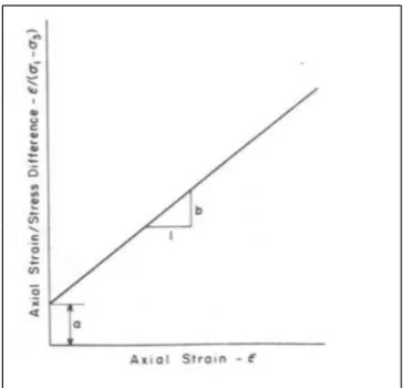
This section summarizes the Hyperbolic model. In 1963, Kondner proposed using the Hyperbolic constitutive model for cohesive soil (Kondner, 1963). Duncan and Chang in their publication, “Non-linear analysis of stress and strain in soils,” indicated that the stress and strain relationship in soils could be better estimated by considering a hyperbolic equation. As shown in figure 1.1, the stress–strain curve in the drained triaxial test can be estimated accurately by a hyperbola (Kondner, 1963). The stress–strain approach in a triaxial test is compatible with a two-constant hyperbolic equation (equation 1.1) (Duncan et Chang, 1970):

− = _. (1.1)

where − is the deviator stress, and and are the major and minor principal stresses, respectively. is the axial strain, and constants a and b are material parameters (Kondner, 1963).

Figure 1.1 Comparison of typical stress and strain curve with hyperbola (Al-Shayea et al., 2001)

(34)

The constants, a and b, will be more understandable if the stress–strain data are drawn on transformed axes as shown in figure 1.2. The parameters a and b are the intercept and slope of the straight line, respectively. In 1970, Duncan and Chang extended the hyperbolic constitutive model in conjunction with confining pressure and several other parameters (Duncan et Chang, 1970).

Figure 1.2 Transformed Hyperbolic stress- strain curve (Duncan et Chang, 1970)

The initial tangent modulus is defined below:

= ( ) (1.2) where pa is the atmospheric pressure, k is a modulus number, and n is the exponent

determining the rate of variation of Ei with . By substituting the parameters a and b, equation 1.1 can be rewritten as

( − ) =

( )

(35)

7

where ( − ) is the deviator stress; and are the major and minor principal stresses; is the axial strain; Ei is the initial tangent modulus, and ( − ) is the ultimate deviator stress.

The hyperbola is supposed to be reliable up to the actual soil failure, which is denoted by point A in figure 1.1 (Al-Shayea et al., 2001). The ratio failure is defined as the proportion between the actual failure deviator stress ( − ) and the ultimate deviator stress( −

) , as indicated in equation 1.4.

= (₍ )₎ (1.4)

The variation of the deviator stress with confining stress can be represented by the well-known MC relationship as indicated in equation 1.5.

( − ) = (1.5)

where c is the cohesion, and is the friction angle.

In addition, Duncan and Chang represented the tangent Young’s modulus as

= 1 − ( )( ) . ( ) (1.6)

Wong and Duncan in 1974 developed the previous works by adding other parameters related to the Poisson’s ratio. Totally, nine parameters, which are listed in table 1.1, are defined.

(36)

Table 1.1 Summary of Hyperbolic parameters (Wong et Duncan, 1974)

Parameter Name Function

K, Kur Modulus number Relate Ei and Eur to

n Modulus exponent

c Cohesion intercept Relate ( − ) to

Friction angle

Rf Failure ratio Relate( − ) to

( − )

G Poisson’s ratio parameter Value of at =

F Poisson’s ratio parameter Decrease in for tenfold increase in

d Poisson’s ratio parameter Rate of increase of with strain

The Mohr envelopes for most of the soils are curved as shown in figure 1.3. Specifically for cohesionless soils, such as rockfills or gravels, this curvature makes it hard to choose a single value of the friction angle, which can be illustrative of the whole range of pressures of interest. To overcome such difficulty, the friction angle can be calculated for values that change with confining stress using equation 1.7 (Wong et Duncan, 1974).

= − ∆ (1.7)

where is the value of for equal to pa, and ∆ is the reduction in for a tenfold increase in . The values of obtained from equation 1.7 are used in equation 1.6 to determine the tangent modulus (Wong et Duncan, 1974).

(37)

9

Figure 1.3 Mohr envelope for Oroville dam core material (Wong et Duncan, 1974)

The variation of axial strain with radial strain can be calculated by means of a hyperbolic equation, i.e., equation 1.8 (Naylor, 1975).

− = (1.8)

In the equation above, is the initial Poisson’s ratio when the strain is zero, and d is a parameter representing the changes in the value of Poisson’s ratio with the radial strain. Figure 1.4 shows the variation of with . In addition, Poisson’s ratio can be estimated for values that vary with the confining stress using equation 1.9.

= − ( ) (1.9)

where is the value of for equal to pa, and is the reduction in Poisson’s ratio for a tenfold increase in (Naylor, 1975).

(38)

Figure 1.4 Hyperbolic axial strain – radial strain curve (Wong et Duncan, 1974)

Moreover, the volume change behavior of soils can be modeled by the bulk modulus, which varies with the confining pressure (Duncan, Wong et Mabry, 1980).

The following equation was presented by Duncan (1980) to calculate bulk modulus.

= (1.10)

where Kb and m are bulk modulus parameters. These parameters can be used instead of the Poisson parameters given in table 1.1.

(39)

11

Equation 1.11 expresses the relationship between the bulk modulus and Poisson’s ratio (Duncan, Wong et Ozawa, 1980):

= (1.11)

Table 1.2 Summary of Hyperbolic parameters (Duncan, Wong et Mabry, 1980)

Parameter Name Function

K, Kur Modulus number Relate Ei and Eur to

n Modulus exponent

c Cohesion intercept Relate ( − ) to

,∆ Friction angle parameters

Rf Failure ratio Relate ( − ) to

( − )

kb Bulk modulus number Value of B/pa at =

m Bulk modulus exponent Change in B/pa for tenfold

increase in

In addition, several finite element programs, such as ISBILD and FEADAM (Duncan, Wong et Ozawa, 1980; Naylor, 1975; Ozawa et Duncan, 1973) were developed to predict the behavior of rockfill dams. The hyperbolic model, as a popular constitutive model, is used to suitably estimate the non-linear and stress dependent stress–strain properties of soils in these programs (Duncan, Wong et Ozawa, 1980; Naylor, 1975; Ozawa et Duncan, 1973).

(40)

Figure 1.5 Variation of bulk modulus with confining pressure (Duncan, Wong et Mabry, 1980)

The soil stress–strain relationship for each load increment of the analysis is considered to be linear. The relation between stress–strain is supposed to obey Hook’s law of elastic deformation. ∆ ∆ ∆ = ( )( ) (1 − ) 0 (1 − ) 0 0 0 (1 − 2 )/2 ∆ ∆ ∆ (1.12)

where ∆ , ∆ , and ∆ are stress increments during a step of the analysis, and ∆ , ∆ , and ∆ are the corresponding strain increments. Et is the tangent Young’s modulus and is the tangent Poisson’s ratio. During each step of the analysis, the value of Et and will be adjusted with calculated stresses in elements (Seed, Duncan et Idriss, 1975).

By considering the bulk modulus, the stress–strain relationship (equation 1.12) can be rewritten as (Duncan, Wong et Mabry, 1980):

(41)

13 ∆ ∆ ∆ = (3 + ) (3 − ) 0 (3 − ) (3 + ) 0 0 0 ∆ ∆ ∆ (1.13)

where E is the stiffness modulus and B is the bulk modulus.

The major inconsistencies of the Hyperbolic constitutive model are specified by Seed et al. (Seed, Duncan et Idriss, 1975) as follows:

1- Since the Hyperbolic model is based on Hook’s law, it cannot show accurately the soil behavior at and after failure when a plastic deformation occurs.

2- The constitutive model does not take into account volume changes owing to shear stress or “shear dilatancy.”

3- The soil model parameters are not fundamental soil properties but are empirical parameter coefficients that depict the soil behavior such as water content, soil density, range of pressure during testing, and drainage on limited conditions. These parameters vary as the physical condition changes.

The advantages of the Hyperbolic constitutive model are listed below (Seed, Duncan et Idriss, 1975):

1- The conventional triaxial test can be used to determine the parameter values.

2- “The same relationships can be applied for effective stress and total stress analyses”. 3- Parameter values can be achieved for different soils; this information can be used in

cases where the available data are not sufficient for defining the dam parameters.

1.2.2 Hardening soil model

The formulation of the HS model is based on the Hyperbolic model as indicated in equation 1.14 (Schanz, Vermeer et Bonnier, 1999). However, the HS soil model has some advantages compared to the Hyperbolic model, such as using the theory of plasticity, allowing for soil

(42)

dilatancy, and considering the yield cap (Brinkgreve et Broere, 2006). Equation 1.14 indicates the relation between the axial strain, and deviatoric strain shown in figure 1.6.

For q<qf = (1.14)

where q is the deviatoric stress. The ultimate deviatoric stress, qf and the asymptotic value of the shear strength, qa are shown in figure 1.6. is the confining stress-dependent stiffness modulus, which can be calculated using equation 1.15:

= , (1.15)

is the secant stiffness in standard drained triaxial test and corresponds to the reference confining pressure. The quantity of stress dependency is defined by the power m (Brinkgreve et Broere, 2006). The value of m is considered equal to 0.5 (Janbu, 1963) while Von Soos (Soos et Bohac, 2001) reported different values in the range between 0.5 and 1.

Figure 1.6 Hyperbolic stress-strain relationship for a standard drained triaxial test in primary loading (Brinkgreve et Broere, 2006)

(43)

15

The ultimate deviatoric stress, qf and asymptotic stress, qa shown in figure 1.6, are calculated

using equations 1.16 and 1.17:

=( − .₎ _(1.16)

= (1.17)

In the equations above, Rf is the failure ratio. C, , and . are the cohesion, friction angle, and minor principal stress, respectively.

Another stiffness, Eur is defined for unloading and reloading stress path as indicated in equation 1.18.

= , (1.18)

where is the reference Young’s modulus that corresponds to the reference pressure for unloading and reloading.

The oedometer stiffness is defined by equation 1.19:

= , (1.19)

where is a tangent stiffness modulus at a vertical stress of = as shown in figure 1.7.

(44)

Figure 1.7 Explanation of in the oedometer test (Brinkgreve et Broere, 2006)

The hardening yield function for shear mechanism is defined as

= ̅ − (1.20)

where ̅ is a function of stress, and is a function of the plastic strain, as indicated in equations 1.21 and 1.22, respectively (Brinkgreve et Broere, 2006).

̅ = − (1.21)

where q is the deviatoric stress, and qa is the asymptotic value of the shear strength. Eur and E50 are the unloading and reloading stiffness and the secant stiffness modulus, respectively, as indicated in equations 1.15 and 1.18.

= − −

= + +

(45)

17

where

is the axial plastic strain. The plastic volume change, is relatively small (Brinkgreve et Broere, 2006; Obrzud, 2010); therefore, for the equation above, we can assume ≈ 2 .

The axial elastic strain is approximated using equation 1.23:

= (1.23) Considering the yield condition = 0, we have ̅ = .

= ̅ = − (1.24)

Combining equations 1.23 and 1.24 will lead to equation 1.25. For the triaxial test, the axial strain is the summation of the elastic and plastic components as indicated in equation 1.25.

= + = + − = (1.25)

The shear plastic strain is given by equation 1.22. The volumetric plastic strain is explained as follows. The plastic flow rule is derived from the plastic potential defined by equation 1.26 (Obrzud, 2010). The rate of plastic volumetric strain for triaxial test can be calculated using equation 1.27, and as can be observed, the relationship is linear.

= + Ψ (1.26) = Ψ (1.27)

where is the mobilized dilatancy angle and can be calculated using the following equation:

(46)

where

is the mobilized friction angle:

sinφ = (1.29) φ is the critical state friction angle, and is defined as

φ = (1.30)

The HS model considers the dilatancy cut-off. While dilating materials after an extensive shearing reach a state of critical density, dilatancy arrives at an end as shown in figure 1.8. To define this behavior, the initial void ratio, einit, and the maximum void ratio, emax for materials should be assigned. When the maximum void ratio appears, the mobilized dilatancy angle, Ψmob, is set to zero (Brinkgreve et Broere, 2006).

For e<emax

Ψ = (1.31) φ = (1.32)

For e>emax Ψ = 0

Equation 1.33 shows the relationship between void ratio and volumetric strain.

(47)

19

Figure 1.8 Dilatancy cut-off (Brinkgreve et Broere, 2006)

The shear yield surface, which is shown in figure 1.9, does not consider the plastic volume strain calculated in isotropic compression. Hence, “a second yield surface is assumed to close the elastic region in the direction of p axis (figure 1.9). This cap yield surface, makes it possible to formulate a model with independent parameters, and ” (Brinkgreve et Broere, 2006). The shear yield surface is regulated by the triaxial modulus, , and the oedometer modulus, , controls the cap yield surface. The yield cap is defined as (Brinkgreve et Broere, 2006):

= ~ + − (1.34)

where pp is the preconsolidation stress. is an auxiliary parameter, which is related to , the normally consolidated coefficient of lateral earth pressure. Other parameters in the equation above are defined as

= −( ) (1.35)

~ ₌ _{+ ( − 1)} _{− ( ) (1.36)}

(48)

Figure 1.9 shows the simple yield lines and figure 1.10 shows the yield surfaces in the principal stress space. “The shear locus and yield cap have hexagonal shapes in the MC model” as shown in figure 1.10 (Brinkgreve et Broere, 2006).

Figure 1.9 Yield surface of the hardening soil model in p-q plane (Brinkgreve et Broere, 2006)

Figure 1.10 The yield contour of the hardening soil model in stress space (Brinkgreve et Broere, 2006)

Mohr-coulomb failure limit-function f, shear yield limit-function

Volumetric yield function

(49)

21

The following advantages of the HS constitutive model are mentioned by Schanz et al. (Schanz, Vermeer et Bonnier, 1999):

1- “In contrast to an elastic-perfectly plastic model, the yield surface of the HS model is not constant in the principal stress space; it can expand owing to plastic straining”. 2- The HS model comprises two types of hardening, that is, shear hardening and

compression hardening. Shear hardening is applied to simulate irreversible strain caused by primary deviatoric loading. Compression hardening is applied to simulate irreversible plastic strain caused by primary compression in oedometer loading. The HS constitutive model limitations are listed below (Obrzud et Eng, 2010):

1- The model is not capable of reproducing softening impacts.

2- The model cannot reproduce the hysteretic soil behavior during cyclic loading.

3- The model considers elastic material behavior during unloading and reloading, while the strain range in which the soil can behave as elastic is considerably small and limited.

1.2.3 Hardening soil-small strain model

The HSS model is a revision of the HS model that considers the increased stiffness of soils at small strains. Generally, soils show more stiffness at small strains when compared with stiffness at engineering strains, as shown in figure 1.11. The stiffness at small strain levels changes non-linearly with strains. The HSS model uses almost the same parameter as the HS model. Two additional parameters i.e. G and _. are required to define the HSS model, where is the small strain shear modulus, and _. is the strain level at which the shear modulus has reduced to 70% of the small strain shear modulus (Brinkgreve et Broere, 2006). As an enhanced version of the HS model, the HSS model can account for small strain stiffness and it is capable to reproduce hysteric soil behavior under cyclic loading conditions (Obrzud, 2010).

(50)

Figure 1.11 Schematic presentation of the HS model, stiffness-strain behavior (Obrzud, 2010)

(51)

CHAPTER 2

COMPARISON AMONG DIFFERENT CONSTITUTIVE SOIL MODELS THROUGH TRIAXIAL AND OEDOMETER TESTS

2.1 Introduction

Choosing an appropriate soil constitutive model is one of the most important elements of a successful finite element or finite difference analysis of soil behavior. There are several soil constitutive models; however, none of them can reproduce all aspects of real soil behavior (Brinkgreve, 2007). In this chapter, various constitutive soil models, namely, Duncan–Chang, MC, HS, and HSS are studied through triaxial and oedometer tests. Two finite element software, Plaxis and Zsoil, are used for the numerical tests. The triaxial and oedometer numerical simulation procedures using Plaxis and Zsoil are explained in sections 2.3 and 2.8, respectively. The studies have focused on Hostun sand (Benz, 2007; Brinkgreve et Broere, 2006; Obrzud, 2010). The standard drained triaxial test is conducted on loose and dense specimens, and experimental tests results are shown in figures 2.4 to 2.6. Finally, the data obtained from Plaxis, Zsoil, and experimental tests are compared with each other.

2.2 Triaxial test

The triaxial test is one of the most popular and reliable methods for calculating soil shear strength parameters. In this test, a specimen that has experienced confining pressure by the compression of fluid in triaxial chamber is subjected to continuously rising axial load to observe the shear failure. This stress can be loaded using two methods. The first method is a stress-controlled test wherein the dead weight is increased in equal increments until the specimen fails. In this method, the axial strain due to the load is measured using a dial gauge. The second method is a strain-controlled test, where the axial deformation is increased at a constant rate. Based on drainage, three types of tests are defined, namely, consolidated-drained, consolidated-unconsolidated-drained, and unconsolidated-undrained (Das et Sobhan, 2013). In this study, the implemented simulations are conducted in consolidated-drained condition.

(52)

2.3 Finite element modeling

In this section, the consolidated-drained triaxial test is modeled and the geometry and boundary conditions, which are used to simulate the model through Plaxis and Zsoil, are presented.

2.3.1 Geometry of model and boundary conditions in Plaxis

A consolidated-drained triaxial test was implemented on the geometry shown in figure 2.1. An axisymmetric model was used. The left and bottom sides of the model were constrained in the horizontal and vertical direction, respectively. The rest of the boundaries were assumed free to move. For simplicity, a 1 m × 1 m unit square was used to simulate the test; these dimensions are not real. This model represents a quarter of the specimen test. As the soil weight was not considered, the dimensions of the model had no impact on the results. The initial stress and steady pore pressure were not taken into account. Furthermore, the deviator stress and confining pressure were simulated as uniformly distributed loads (Brinkgreve, 2007).

(53)

25

In the first phase, the model was exposed to a confining pressure, = −300 kPa to allow consolidation. In the second stage, the model was loaded vertically up to failure, whereas the horizontal confining pressure was kept unchanged.

A fifteen-node triangular element was used. It is crucially important to use a sufficient number of refined meshes to ensure that the results from the finite element software are precise. To observe the influence of mesh size on the stress–strain graph, several analyses were implemented using Plaxis. Table 2.1 shows that decreasing the mesh size has no significant influence on the maximum deviatoric stress. As the modeled test has a relatively simple geometry, decreasing the mesh size has no significant influence on the test results (Brinkgreve, 2007).

(54)

Table 2.1 Mesh size influences on deviatoric stress for the Hardening soil model in Plaxis software

Average element size (mm)

Number of nodes Maximum deviatoric stress

91.29 1017 1164.98

61.78 2177 1165.75

41.81 4689 1165.75

2.3.2 Geometry of model and boundary condition in Zsoil

A compressive triaxial test can be simulated by using an axisymmetric geometry of unit dimension, 1 m × 1 m, that represents a quarter of the soil sample (Brinkgreve, 2007). As the weight was not considered, the dimensions of the model had no impact on the results. The initial stresses were set to a uniform compressive pressure of 300 kPa for all three directions to account for the consolidation under confining pressure. As the strain control test was performed, the load was imposed as vertical displacement on the top nodes while the bottom nodes were fixed in the vertical direction. The displacement magnitude of top nodes was defined as a load–time function. Horizontal confining pressure was applied on the right side, while the left side was kept fixed horizontally. Various mesh sizes were used to model the test; however, as can be observed in table 2.2, refining the mesh size has no significant influence on the results owing to the relatively simple geometry of the triaxial test. Four-node quadrilateral elements were used for meshing as shown in figure 2.3.

(55)

27

Figure 2.3 Plot of the mesh in Zsoil

Table 2.2 Mesh size influences on deviatoric stress for the Hardening soil model in Zsoil software

Number of elements Number of nodes Maximum deviatoric stress

1 4 1144.49 81 100 1144.51 729 784 1144.52

2.4 Experimental data

Experimental data on dense and loose Hostun sand available from reports (Benz, 2007; Brinkgreve et Broere, 2006; Obrzud, 2010) were used to obtain the parameters. Consolidated-drained triaxial tests at a fixed pressure of = −300 kPa were conducted on loose and dense sand. Furthermore, four control tests were performed to check the possibility of reproducing the test results (Schanz et Vermeer, 1996). The results are shown in figures 2.4 and 2.5, where the deviatoric stress-axial–strain and volumetric strain-axial–strain curves are illustrated. As shown, the reproducibility of results is satisfactory (Schanz et Vermeer, 1996).

(56)

Figure 2.4 Results of drained triaxial test on loose Hostun sand (Brinkgreve, 2007)

Figure 2.5 Results of drained triaxial test on dense Hostun sand, deviatoric stress versus axial strain (Brinkgreve et Broere, 2006)

(57)

29

Figure 2.6 Results of drained triaxial test on dense Hostun sand, volumetric strain versus axial strain (Brinkgreve et Broere, 2006)

2.5 Application of constitutive soil models

The stress–strain relationship for Hostun sand was modeled using various constitutive models in Plaxis and Zsoil. The results of Zsoil and Plaxis for different models were compared with experimental data, as shown in figures 2.4 to 2.6, to determine the most appropriate model.

2.5.1 Mohr–Coulomb model

The MC model is a linear elastic-perfectly plastic model used to depict the soil response when subjected to shear stress (Ti et al., 2009). The linear region is based on Hooke’s law of isotropic elasticity, while the plastic region is attributed to the MC failure criterion (Ti et al., 2009). Five parameters are required to define the MC soil model (table 2.3). For real soil, the stiffness modulus is not constant and depends on the stress. E0 is the initial stiffness and E50

is the secant modulus at 50% of the soil strength as shown in figure 2.7. For a material with an extended elastic range, using the initial stiffness, E0 seems appropriate; however, using E50

(58)

for loading of soils is generally acceptable (Brinkgreve et Broere, 2006). E50 is used for this modeling. For the MC model in many cases, it is suggested to consider a Poisson’s ratio between 0.3 and 0.4 (Brinkgreve et Broere, 2006); hence a Poisson’s ratio of 0.35 is assumed.

Figure 2.7 The initial stiffness, E0 and the secant

modulus, E50 (Brinkgreve et Broere, 2006)

Table 2.3 Soil properties used in the MC model for loose sand

Material Model Data group Properties Unit Value

Hostun loose sand Mohr-Coulomb Elastic E [KN/m2_{] 20000} - 0.35 Density [KN/m3_{] 17} [KN/m3_{] 10} Nonlinear [degree] 34 [degree] 0 C [KN/m2_{] 0}

(59)

31

Table 2.4 Soil properties used in the MC model for dense sand

Material Model Data group Properties Unit Value

Hostun dense sand Mohr-Coulomb Elastic E [KN/m2_{] 37000} - 0.35 Density [KN/m3_{] 17.5} [KN/m3_{] 10} Nonlinear [degree] 41 [degree] 14 C [KN/m2_{] 0}

Numerical analyses conducted on the MC model are shown in figures 2.8 to 2.11. This model consists of elastic and plastic portions. The results shown in figures 2.8 to 2.11 do not indicate good agreement between experimental tests and simulated results. The experimental result shows a curved shape, whereas the MC simulation result in the elastic part is linear (figures 2.8 and 2.10). Consequently, the simulation implemented using the MC model cannot demonstrate softening behavior in dense sand as shown in figure 2.8. Simulation results and experimental results for loose sand as shown in figure 2.10 are more compatible. Finally, it can be clearly observed that the simulation results using Plaxis and Zsoil (figures 2.8 to 2.11) are in agreement.

(60)

Figure 2.8 Deviatoric stress vs axial strain for the MC model in dense sand

(61)

33

Figure 2.10 Deviatoric stress vs axial strain for the MC model in loose sand

(62)

2.5.2 Hardening soil model

In this section, the HS model is used to simulate the drained triaxial test. In contrast to the MC model, the soil stiffness in this model is defined more precisely by using three modulus stiffnesses, namely, the triaxial loading stiffness, triaxial unloading stiffness, and oedometer loading stiffness (Brinkgreve, 2007). A summary of the HS model parameters for Hostun sand is presented in table 2.5.

Table 2.5 Soil properties used in the HS model for dense and loose sand (Brinkgreve, 2007) Material Model Properties Unit Dense sand Loose sand

Hostun sand Hardening [KN/m2_{] 37000 20000}

[KN/m2_{] 90000 60000} [KN/m2_{] 29600 16000} ϑ - 0.2 0.2 [KN/m3_{] 17.5} ₁₇ [KN/m3_{] 10} ₁₀ [degree] 41 34 [degree] 14 0 C [KN/m2_{] 0} ₀ m - 0.5 0.65 Failure ratio - 0.9 0.9 - 0.34 0.44

(63)

35

The theoretical solution for failure of a sample is calculated based on the MC model (equation 2.1):

=| |+ sin − . cos = 0 (2.1) The failure due to compression is calculated as

For dense soil = . − 2 . =1455.8 (2.2) | − | = 1155.8

For loose soil = . − 2 . = 1063 | − | = 763

The confining pressure, is assumed as 300 kPa. The deviator stress values ( − ) for dense and loose sand, calculated theoretically using equation 2.2, are in good agreement with the results of Plaxis, Zsoil, and the results obtained from experimental tests.

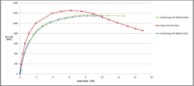
As shown in figure 2.12, for both experimental test data (dense Hostun sand) and numerical analysis conducted based on the HS constitutive model, a hyperbolic relationship can be observed between the deviatoric stress (principal stress difference) and the vertical strain. The stress–strain relationship of soil in the HS model before reaching failure is based on the hyperbolic model (Schanz, Vermeer et Bonnier, 1999). A good agreement is indicated in figure 2.12 between the first hyperbolic part of the simulation conducted using Plaxis and Zsoil and the experimental data. The HS model does not include any softening behavior (Obrzud et Eng, 2010); hence, the second part of the graph stays constant and cannot completely show the same experimental results. In figure 2.14, it can be observed that the triaxial test results (for loose Hostun sand) based on the HS constitutive model calculation are in good agreement with experimental test results. Finally, it is evident that the ultimate shear strength for dense sand is higher than loose sand; this can be observed in figures 2.12 and 2.14. A good agreement is observed between Plaxis and Zsoil test results.

(64)

Figure 2.12 Deviatoric stress vs axial strain for the HS model in dense sand

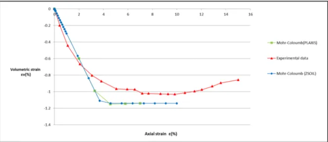
Figures 2.13 and 2.15 show the volumetric strain versus axial strain. Dilation can be observed in figure 2.13 for dense sand, where sand particles are moved out of voids due to increasing shear force. In figure 2.15, negative dilation can be observed as sand particles continue to move into larger voids until failure (Towhata, 2008).

(65)

37

Figure 2.14 Deviatoric stress vs axial strain for the HS model in loose sand

(66)

2.5.3 Hardening small strain soil model

In this section, the HSS model is studied to simulate the soil behavior in drained triaxial tests. For HSS modeling, two extra parameters are required apart from those required in the HS model; their values are given in table 2.6.

Table 2.6 Supplemental HS Small soil parameters for loose and dense Hostun sand (Brinkgreve, 2007)

Parameters Loose sand Dense sand

G0ref(pref=100kpa) 70000 112500

Shear strain 0.0001 0.0002

For loose sand (figure 2.18), the deviatoric stress increases with axial strain until a failure shear stress is reached. After reaching that point, the shear resistance is approximately constant with further increase in axial strain. In dense sand (figure 2.16), the deviatoric stress rises with increasing axial strain before reaching the peak stress after which a decrease in deviatoric stress is observed. The analysis implemented using the HSS soil model can reproduce the same trends except the softening behavior in dense sand. Furthermore, a good agreement was found between Plaxis and Zsoil results.

(67)

39

Figure 2.16 Deviatoric stress vs axial strain for the HSS model in dense sand

Increase in shear force is often accompanied by an increase in volume of the system for dense sand, which is referred to as dilatancy. This is the result of change in alignment of soil particles. An increased shear force moves the soil particles inside the voids resulting in a decrease of volume or negative dilatancy as can be observed in figure 2.19 and the starting region in figure 2.17 (Towhata, 2008). For dense sand, as the shear force continues to rise, the particles instead of being pushed in are pushed out of the intergranular spaces leading to increase in volume of the system (Towhata, 2008) as can be observed in figure 2.17. Since the HSS model accounts for dilatancy, it can be observed in the result of Zsoil and Plaxis (figures 2.17 and 2.19). Zsoil correctly shows dilatancy in dense and loose sands and has an acceptable deviation from the real test results.

(68)

Figure 2.17 Volumetric strain vs axial strain for the HSS model in dense sand

(69)

41

Figure 2.19 Volumetric strain vs axial strain for the HSS model in loose sand

2.5.4 Duncan–Chang soil model

In this section, the Duncan–Chang soil model is used to simulate the drained triaxial test. This constitutive soil model is a non-linear elastic model based on a hyperbolic stress–strain relationship. The parameters employed to depict the hyperbolic stress–strain relation are k (modulus number), n (modulus exponent), Rf (failure ratio), and G, F, d (Poisson’s ratio parameters). A summary of the Duncan–Chang soil model parameters for Hostun sand is presented in table 2.7.

(70)

Table 2.7 Soil properties used in the model for dense and loose sand

Material Model Properties Unit Dense sand Loose sand Hostun sand

Duncan-Chang [KN/m3] 17.5 17 [KN/m3] 10 10 [degree] 41 34 C [KN/m2] 0 0 n - 0.5 0.65 Rf (Failure ratio) - 0.8 0.8 - 740 400 G - 0.3065 0.38 F - 0.02 0.013 d - 9.24 3.85

Numerical analyses implemented on the Duncan–Chang model are shown in figures 2.20 to 2.23. The confining pressure, is assumed as 300 kPa. For both experimental test data (dense Hostun sand) and numerical analysis, a hyperbolic relationship can be observed between the deviatoric stress (principal stress difference) and the vertical strain (figure 2.20). The Duncan–Chang model was formulated in order to exhibit an appropriate and fit result on the data. A good agreement is indicated in figure 2.20 between the first hyperbolic part of the simulation conducted using Zsoil and experimental data.

The Duncan–Chang soil model does not include softening behavior; hence, the second part of the graph cannot completely depict the experimental results. From figure 2.22, it can be observed that the simulations (for loose Hostun sand) closely agree with experimental test results.

For the volumetric strain versus axial strain, it is shown that the simulation cannot describe the soil volumetric–axial strain relation for dense sand (figure 2.21). As the Duncan–Chang

(71)

43

soil model does not consider dilatancy parameter, a remarkably large difference can be observed between the simulation and experimental data.

Figure 2.20 Deviatoric stress vs axial strain for the Duncan-Chang model in dense sand