Science Arts & Métiers (SAM)
is an open access repository that collects the work of Arts et Métiers Institute of Technology researchers and makes it freely available over the web where possible.
This is an author-deposited version published in: https://sam.ensam.eu Handle ID: .http://hdl.handle.net/10985/14695
To cite this version :
Vlasios LEONTIDIS, Christophe CUVIER, Guy CAIGNAERT, Patrick DUPONT, Olivier ROUSSETTE, Simon FAMMERY, P. NIVET, Antoine DAZIN - Experimental validation of an ultrasonic flowmeter for unsteady flows - Measurement Science and Technology - Vol. 29, n°4, p.045303 - 2018
Any correspondence concerning this service should be sent to the repository Administrator : [email protected]
1
Experimental validation of an ultrasonic flowmeter for
unsteady flows application
V Leontidis1, C Cuvier2, G Caignaert1, P Dupont1, O Roussette1, S Fammery3, P Nivet3 and A Dazin1
1
Ecole Nationale Supérieure d’Arts et Métiers, Laboratoire de Mécanique de Lille, FRE CNRS 3723 Lille, France
2
Ecole Centrale de Lille, Laboratoire de Mécanique de Lille, FRE CNRS 3723 Lille, France
3
Ariane Group, Vernon, France E-mail: [email protected]
Abstract. An ultrasonic flowmeter has been developed for further applications in cryogenic conditions and for measuring flow rate fluctuations in the range of 0 to 70 Hz. The prototype was installed in a flow test rig and was validated experimentally both in steady and unsteady conditions for water flows. A Coriolis flow meter was used for the calibration under steady state conditions, whereas in the unsteady case the validation was done simultaneously against two methods, the particle image velocimetry (PIV) and with pressure transducers flush installed on the wall of the pipe. The results show that the developed flowmeter and the proposed methodology can accurately measure the frequency and the amplitude of the unsteady fluctuations in the experimental range of 0-9 l/s of the mean main flow rate and 0-70 Hz of the imposed disturbances.
Keywords. Unsteady flows, ultrasonic flowmeter, particle image velocimetry, pressure transducer
1. Introduction
It is very common in several technical and industrial applications flows of liquids to occur under non-ideal conditions or to deviate from the design conditions, and as a result the flow to be disturbed. Typical examples can be found in fluid turbomachinery (e.g. each row produces a non-uniform outlet flow field) [1], in oil industry (e.g. custody transfer of petroleum products) [2]. The origin of the unsteadiness can be either because of non-ideal flow distribution across the flow cross section (i.e. an asymmetric velocity profile or a not fully developed flow) or because the flow is unsteady (i.e. the flow rate is pulsating or existence of secondary flows) [3]. The performance of many types of flowmeters and the installation effects of typical flow disturbances have been extensively studied [4-10]. Thus, it becomes obvious that the accurate determination of liquid flow rates is an open research field and can be considered crucial both for safety and economic reasons since it can lead to better
2 design of systems, ensuring the operation under optimal conditions, and preventing of unexpected phenomena (i.e. cavitation, shut down).
Many methods have been developed, proposed, and applied for steady measurements, and some of them have been used or have been modified in order to be used under transient conditions. In the selection of the appropriate flowmeter several factors must be considered in priory mainly having to do with the application, i.e. physical properties, operation conditions, location, price, and others [11]. Generally, the flow measurement techniques can be split into two major categories:
• Non-intrusive flowmeters causing no additional head losses:
o Electromagnetic or ultrasound flowmeters
o Use of pressure transducers flush mounted on the walls of a pipe
o Optical methods such as LDV (Laser Doppler Velocimetry) or PIV (Particle Image Velocimetry)
• Flowmeters introducing higher head losses:
o Use of transducers inside the flow (Pitot tube, hot wire or hot film velocimetry)
o Venturi, diaphragm, turbine, Coriolis flowmeters
Measurements in unsteady pulsating flows (regular cyclic variation in flow velocity superimposed on a constant time-average flowrate) [12] have already been performed with several techniques and the effect on the flow rate reading has been documented, such as in Coriolis flowmeter [13,14], vortex flowmeter [15,16], ultrasonic gas flowmeter [17], orifices plates [18], Venturi [19], hot-wire anemometry [20,21].
The present study refers to applications in the field of hydraulic machinery and has been exclusively done using water at room temperature. The objective was clearly to focus on non-intrusive methods as well as no head loss methods. For practical use the PIV and LDV methods cannot be considered as a solution of the problem under investigation. However, they can be used as reference methods in a research laboratory.
Two types of unsteady flows can be encountered in such applications, where the fluid is nearly incompressible and generally characterized by high Reynolds number:
• Transient behavior of pumps and turbines.
o The use of an electromagnetic flowmeter has been proposed [22] for fast start-up tests of a radial flow pump in water with a frequency resolution of data acquisition equal to 5 kHz.
o The use of pressure transducers flush mounted on the wall of pipes has been also used for the same kind of study [23], with a measurement frequency of around 8 kHz.
• The analysis of instabilities associated, for example, with:
o interactions between machines and systems in partial flow rates conditions such as the POGO oscillations caused by combustion instabilities in liquid propellant rocket engines [24,25] or
o forced excitations with external devices [26-28] in order to access to an experimental characterization of natural frequencies of hydraulic systems: a minimum of two pressure transducers flush mounted on the wall in pipes is mainly used to access to the flow rate fluctuations, using adequate hydro-acoustic models [26].
Regarding non-intrusive and no-head loss methods, two types of flowmeters can be proposed: electromagnetic (denoted as EM) and ultrasonic (denoted as US). The EM flowmeter has already been used [29], with a necessary adaptation of the electronic of the system in order to access to the convenient time response. But it is well known that its use is limited to conducting fluids, for example water containing ions, and requires an electrical insulating pipe surface, for example a rubber-lined
3 steel tube. These restrictions are limitations when cryogenic applications are considered. That’s why the present study is focused on the use and extension of an US flowmeter.
Ultrasonic flowmeters are one of the fastest-growing technologies within the general field of instruments for process monitoring, measurement, and control [30]. Three of the most common types of ultrasonic flow meters are: the Doppler (reflection) [31-33], the transit time (time-of-flight) and the cross-correlation [34] flowmeter. Compared with the traditional technologies, transit-time ultrasonic flowmeter possesses many advantages [30]:
• high accuracy and reproducibility,
• no moving parts,
• no extra pressure drop,
• bi-direction measurements possible, and
• can be conveniently maintained on-line without interrupting the fluid transport. Today, numerous commercial flowmeters are available in the market.
A flow metering system using the US Doppler method (obtaining the instantaneous velocity profiles along the ultrasonic beam) using a single line [35] and multiple lines [36] was developed and tested under transient conditions (non-developed flow below an elbow). However, the specific method demands the existence of particles in the flow (the above authors used cavitation bubbles).
The paper is concerned with the transit time technology (or time-of-flight method, denoted as TOF) in US flow metering. In such a method, the basic principles are the following [37]:
• Two transducers are installed on the wall of the pipe creating a measuring beam
• One transducer acts as an emitter of an acoustic wave, due to an impulsive excitation of an electronic signal, and the second one acts as a receiver of the wave. The measurement of the time delay between emission and reception is a function of the wave celerity of the fluid and a mean axial component of the flow velocity in the duct. It must be noted that the wave celerity is very much higher than the flow velocity (very low Mach number). For accurate determination of the mean flow velocity, and hence of the mean flow rate, conventional US flowmeters use a measurement of the difference of time of flight between the time delays when each transducer is sequentially being used as emitter or receiver. To access to a better accuracy of flow rate measurement, industrial flowmeters use many measuring beams (3 is a rather common value) in each measuring zone [38,39]. The various excitation signals are conventionally applied sequentially, in order to prevent the effects of interferences between the various beams and this of course limits the time response of a conventional US flow meter very much.
It is known that the accuracy of a US flowmeter can be affected by several factors, among which are the occurrence of a pulsating flow, the shape of the flow profile and turbulence, pipe geometry and roughness [40-43]. It is believed that the measurement methodology developed in the present work takes into consideration most of the above limiting factors.
The analysis of the use of the time-of-flight method under fluctuating operating conditions up to 70 Hz, in a prototype multipath ultrasonic flowmeter of water flows in a pipe is the core of the present study. First, a detailed description of the developed ultrasonic flowmeter together with its operation and measurement principle is given. Next, the experimental facility where the flow tests took place, and the tools (instrumentation and methods) that were used and applied during the tests are presented. It is worth mentioning that two alternative experimental methods were used for the evaluation of the prototype and the measurement methodology:
4
• Particle Image Velocimetry (denoted as PIV) in a plane of the flow, and
• Pressure transducers mounted on the wall of the pipe
and for the post-processing of the experimental data (signals from the US flowmeter and the pressure transducers, images from the PIV) in-house routines in MATLAB were developed.
2. The ultrasonic flowmeter prototype
2.1 Concept and components
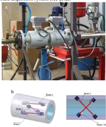
The developed prototype (Figure 1a) is a custom double body ultrasonic flowmeter (denoted as US). In the first body, there are three measuring beams along different chords of the cross-section and not along a diameter (figure 1b), while in the second body, there is only one measuring beam along one diameter of the body. The sensors can be used to measure the speed of waves inside a liquid (cryogenic or not) medium and every beam consists of one transmitter and one receiver. The flowmeter came without external terminal (flow converter) for the input and output signals to be registered with an appropriate acquisition system (see §3.2).
Figure 1. The two-body cryogenic ultrasonic flowmeter (a)
Location of the six sensors and the three measurement lines on the first body (b) Unsteady water flow tests in a pipe were performed in previous series of experiments with a single body 3-beam ultrasonic flow meter in which three separate measuring units have been installed to make it possible to obtain the measurements at every channel. Simultaneous measurements with three pressure sensors mounted on the walls of the pipe (see §3.2) were performed to compare the amplitude and frequency of the imposed fluctuation (see §2.3) and to validate the developed methodology (excitation and acquisition systems, and post-processing). Although the overall methodology showed to be very promising, deviations in the fluctuation amplitude and limitations in the detection of disturbances in low frequencies were observed which were attributed both to the acquisition system and to the weakness of the single body which leads to strong interferences between lines. It was concluded that the use of a double body flowmeter will allow to detect fluctuations with higher accuracy in the range of 0-70 Hz by comparing the signal between sensors from different bodies.
a
5 2.2 Operation principle
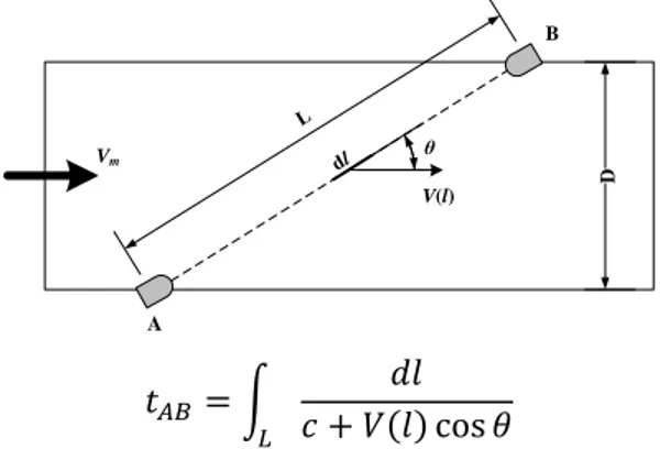
The basic principle is based on measuring the propagation time of an ultrasonic wave to propagate inside a liquid medium from the transmitting to the receiving sensor. The transit time depends both on the fluid and the flow regime in the pipe. The measured transit time is influenced by the velocity of the waves, c, in the fluid, and by the distribution of the axial velocities, V, of the flow along the path of the measurement line, l, according to the integral expression of figure 2. The method commonly used in the ultrasonic flowmeters is to calculate the flow rate from measurements of the above transit time [37].
= + cos
Figure 2. Operation principle of ultrasonic flowmeters
The flow velocity is usually estimated using the transit-time differential method, which is based on the fact that a sound wave travelling in the direction of the flow propagates at a faster rate than one travelling against the flow (tAB < tBA). Transit times tAB and tBA are measured sequentially. The difference (1/tBA - 1/tAB) in time travelled by the two ultrasonic waves is directly proportional to the mean flow velocity, Vm, of the fluid.
However, this method implies that the transducers A & B are playing one after the other the role of the emitter and of the receiver. This is an inherent limitation in the time resolution of this method, which is thus limited to frequencies in the order of several Hz for a standard flowmeter.
2.3 Measurement principle
Transit time ultrasonic flowmeters send and receive ultrasonic waves between transducers in both the upstream and downstream directions in the pipe. Thus, the metrological principle is based on the measurements of the travelling time of a pulse signal generating ultrasonic waves at one resonant frequency of the transducer through the liquid medium; one of the two transducers is used as a transmitter and the other is used as a receiver. The choice of the direction of the generated pulse affects the transit time measurement with respect to the direction of the flow in the pipe.
The manufacturer of the flowmeter recommended applying on the transmitter an excitation pulse with a 250 ns duration and a 100 V maximum amplitude. An in-house tool in LabVIEW environment was developed for the creation of the control signal (figure 3)
D θ B A V(l) Vm
6
Figure 3. Control signal of the excitation of the transmitters of the ultrasonic flowmeter
3. Testing facilities and measurement conditions
3.1 Experimental set-up
The experimental facility (figure 4) was a close loop, which could be pressurized up to 6 bar. A free surface reservoir provides the necessary liquid medium, water at room temperature in the present case. At the bottom of the reservoir (outlet) there was a straight DN40 piping system (total length 3756 mm including all instrumentations and fittings), in which the steady and unsteady state measurements were performed. At the end of the straight part a radial flow pump was used in order to control the flow rate in the system, by modifying its speed of rotation. The outlet of the pump returned to the reservoir.
Figure 4. Flow loop (dimensions in cm)
A secondary open loop existed, in parallel with the closed loop, for the creation of the necessary periodic fluctuations on the liquid flow rate and thus establishing an unsteady flow. This auxiliary circuit was comprised of a 1.9 cm piping and was sucking water from the main installation and discharging the water through a rotary valve of adjustable frequency of rotation. This parallel loop was connected at 560 mm downstream to the tank through a “T” junction with the main loop. A valve was installed to isolate it when necessary.
3.2 Measurement methodology
Four different experimental measurements devices were used:
• Double body ultrasonic flowmeter (denoted as US)
• Coriolis flowmeter (denoted as CF)
• Pressure sensors (denoted as PS)
• Particle image velocimetry (PIV)
The US flowmeter was permanently installed in the loop at a distance equal to 2070 mm from the tank. The input and output signals were registered with an acquisition system delivered by NATIONAL INSTRUMENT.
7 A custom build-in tool in LabVIEW environment was developed for registering the signal from 1 up to 5 channels simultaneously, with a sample frequency high enough in comparison with the natural frequency of the transducers. The same system (hardware and developed software) was used for the excitation of the transmitters of the US. The signals being registered systematically were:
• Channel 0: the excitation signal send on the US emitters (denoted as CH0)
• Channels 1 to 3: the response signals of the US receivers of the first body (denoted as CH1-CH3)
• Channel 4: the response signal of the US receiver of the second body (denoted as CH4)
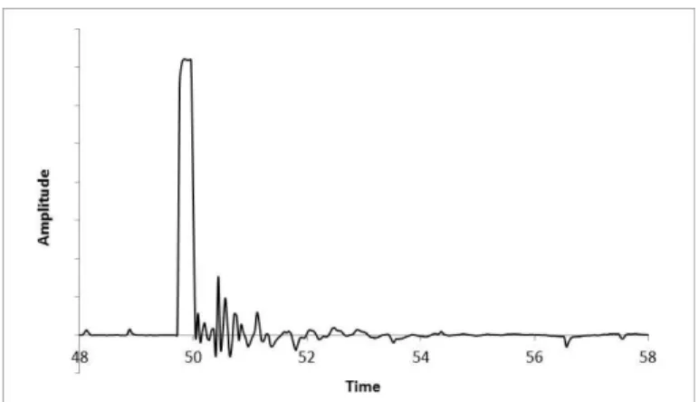
Also, MATLAB routines were developed for transforming and post-processing the recording data. On figure 5 a typical recording of the response of two sensors of the US is being presented.
Figure 5. Superimposed responses of two receivers of the ultrasonic flowmeter
Downstream, 700 mm after the US flowmeter, a curved tube Coriolis flowmeter was installed. The purpose of the CF was to measure the flow rate during the steady state flow tests and to be used as a reference for the calibration of the US flowmeter and the PIV method. The accuracy of the CF (according to the manufacturer) is ±0.05% in the calibrated mass flow range of 1.2-12 kg/s. However, during the dynamic tests the CF was being removed, because the CF was causing significant pressure drop resulting in a reduced maximum flow rate achieved by the pump.
Just after the junction of the secondary loop three piezoelectric pressure sensors were flush mounted on the walls of the pipe of the primary loop, just between the “T” junction and the US flowmeter. Each sensor was connected to a load amplifier delivering an output voltage proportional to the pressure. The commercial acquisition software LMS Test.Lab was used for registering the output signals.
The application of an other non-intrusive reference method for evaluating the amplitudes and frequencies of flow fluctuations was crucial. For that reason, PIV measurements in a transparent pipe, with the same internal diameter with the main pipes, located immediately downstream of the US flowmeter were also carried out. It was assumed that the flow velocity profiles in the two sections (US & PIV) will be similar considering that sufficient straight lengths are being arranged upstream and downstream of this assembly. Measurements were performed in two planes with an offset of 90° between each plane: a vertical one (the camera was placed at the side of the transparent part, denoted as PL1) and a horizontal plane (images were taken from above of the transparent part, denoted as PL2). PIV measurements used:
• a dual oscillator, single head, diode pumped Nd:YLF Laser with a high repetition rate
• a high-speed camera CMOS
• a synchronization between camera and laser
8 The resolution of each captured image was selected as 1216 x 1200 pixels; 1216 pixels along the axis of the pipe and 1200 pixels in the diametric direction, of which 1160 pixels were inside the flow. The time intervals between two images were chosen taking into account the value of the mean flow rate in the pipe. These adjustments provided a good compromise between measurement dynamics and measurement noise. The hardware allowed the recordings of instantaneous flow velocity maps in a plane with a measurement frequency perfectly consistent with the measuring frequency of the US flowmeter. The images were processed with a modified version of MatPIV toolbox under Matlab. First, the images were normalized with the division by the mean background images to minimize the reflections at the walls and to minimize the noise [44]. Then they were processed with a standard multipass–multigrid PIV algorithms [45, 46] with four passes, starting with 64x64 interrogations windows and ending with 24x24 ones. Before the final pass, images deformation was applied to improve the quality of the results [47, 48].
3.3 Experimental protocols
Two series of flow tests were performed for each position of the PIV (PL1 and PL2), in all cases with elevated pressure in the tank (P = 3 bar) in order to establish the higher possible flow rate with no cavitation. Each series consists of two different set of experiments: one test under steady conditions followed by a test with imposed fluctuations.
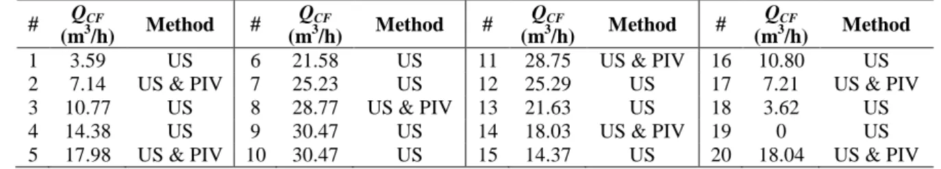
During the steady case the CF was placed on the loop and used as a reference for the calibration of the US flowmeter and the PIV method, while the secondary loop was isolated. The flow rate, Q, was being increased gradually with a step of around 1 l/s up to the maximum value, taking measurements with US at every step, while with the PIV three measurements were carried out simultaneously with US. The same procedure was used, but by decreasing the flow rate for repeatability controls. Two additional operating conditions were acquired with the US: one with no flow in the system and one with a randomly chosen flow rate. Table 1 summarizes the steady state tests. For all three steady state tests (#1 to 9, #10 to 18, #19 to 20), the target flow rate at each step was similar with the values of Table 1, but small deviations occurred.
Table 1. Steady state flow tests and flow rates references
# QCF (m3/h) Method # QCF (m3/h) Method # QCF (m3/h) Method # QCF (m3/h) Method 1 3.59 US 6 21.58 US 11 28.75 US & PIV 16 10.80 US 2 7.14 US & PIV 7 25.23 US 12 25.29 US 17 7.21 US & PIV 3 10.77 US 8 28.77 US & PIV 13 21.63 US 18 3.62 US 4 14.38 US 9 30.47 US 14 18.03 US & PIV 19 0 US 5 17.98 US & PIV 10 30.47 US 15 14.37 US 20 18.04 US & PIV For the unsteady cases the CF was removed. Measurements with the PIV were carried out in two planes of the flow (PL1 and PL2) and the PS were also used. The results of PIV and PS were the basis to be compared with the results of US. Three mean flow rates were used and fluctuations at five frequencies were imposed. Some measurements were repeated to check the repeatability of the US. Before taking each measurement, the flow rate was established on the main loop, then the isolation valve was turned on and the rotary valve on the secondary loop was started. Measurements with the three methods were carried out simultaneously. The developed LabVIEW program was used for triggering all experimental methods, so that the measurements of the different methods were performed simultaneously and for the same duration. Table 2 summarizes the unsteady flow tests of plane 1 and plane 2 of the PIV. The mean flow rates, Qnom, and the frequencies, fnom, included on the table were nominal values: the flow rate was corresponding to a targeting value, while the frequency
9 was roughly estimated at the beginning of each test using the PS measuring system and the commercial software.
Table 2. Unsteady state flow tests and flow rates references
# Qnom (m 3 /h) fnom (Hz) # Qnom (m 3 /h) fnom (Hz) # Qnom (m 3 /h) fnom (Hz) PL1 PL2 PL1 PL2 PL1 PL2 1-3 7.2 8 16 18 8 21-23 28.8 8 4-6 7.2 15 17 18 15 24-26 28.8 15 7-9 7.2 30 18 18 30 27-29 28.8 30 10-12 7.2 50 19 18 50 30-32 28.8 50 12-15 7.2 70 20 18 70 33-35 28.8 70
4. Results and discussion
4.1 Calibration
The measurement of the CF was always being used as a reference for the calibration of US and PIV methods. The experimental points (#1, #18 and #19) that were outside of the range of the CF were not considered for the calibration of the US.
For the US flowmeter, it is always necessary to combine the signal of different receivers but always in pairs. Among the several possibilities it was chosen to present hereafter the results of CH1 & CH4, since the results of all other combinations (CH2 & CH4, CH3 & CH4) were the same and leaded to identical outcomes.
The proposed methodology of the US calibration is based on the definition of the transit times DT1 and DT4.
= t + + (1)
= t + + (2)
These terms are derived from the integral expression of the transit time between a transmitter and a receiver by including in constants k1 and k4 various factors, such as the inclination of the measuring line relative to the axial direction of the pipe, the cross-sectional area, and a consideration of the distribution of the axial components of the flow along the measurement lines L1 and L4, which represents the distance between the transmitter and the receiver. The method used to determine the transit time have been proved to introduce a characteristic time delays, representative of the acquisition system time delay and of the delay induced by the post-processing procedure used to determine the transit times, t1 and t4, which have been included in the equations. It should also be noted that in the case that the beam pair is along the diameter of the flowmeter, like in case of CH4 on the second body, the constant k is theoretically equal to zero since the inclination angle is θ = 90°. If the celerity of waves, c, is equal for the two lines, it can be eliminated by combining the two equations:
= − 1− − − 1− (3)
10
= − 1 + − − 1 + (4)
The evolution of DT1 and DT4 during the flow tests is small, because they depend mainly on wave celerity. Eq. (4) can be rearranged in the following expanded form:
=
!
"−! "
− + − 1 − − 1 (5)
Following the previous remark the first term on the right part of eq. (5) can be assumed to be almost constant. Thus, the bellow equation is being proposed to be used in the calibration procedure:
= # − $ + (6)
where the constants a (expressed in m3), b (in m3), and c (in m3/s) are:
# = − (7)
$ = − (8)
= %− % (9)
The two transit times and associated standard deviations, σ, during the steady state flow tests were found to vary between: DT1 = 4.236×10⁻⁵ – 4.247×10⁻⁵ s, σ1 = 8.65×10⁻⁹ – 1.00×10⁻⁸ s, and DT4 = 2.915×10⁻⁵ – 2.919×10⁻⁵ s, σ1 = 8.76×10⁻⁹ – 9.17×10⁻⁹ s. For the determination of the constants of eq. (6) the least mean square method was applied on the experimental data of the transit times.
On figure 6 the dispersion of the points used to establish the calibration law and the values of the corresponding constants are being presented. The dash line indicates the perfect equality between the flow rates of the reference flowmeter and the flow rate of the ultrasonic flowmeter determined with the calibration law. The 95% confidence interval of the mean values was varying between ±0.116 and ±0.202 m3/h. Similar calculations were also carried out for all pair combinations of the US receivers. Although different values of the constants were obtained, the conclusions were identical. By imposing the calibration curve on the additional measurement points (#18 & #20) the flow rates were predicted by the US with a relative difference of 2.3% at the low flow rate (point #18) and 0.25% at the higher flow rate (point#20), when compared to the CF value.
11
Figure 6. Calibration law of the ultrasonic flowmeter US
Figure 7 shows an instantaneous PIV map of the axial components of flow velocities during steady flow test #2 and a map obtained after averaging all instantaneous maps. The post-processing of the data relating to each map of the mean values of velocities consisted of:
• The determination of an average distribution of axial components of pipe velocities along the diameter (averaging performed by assuming axial uniformity of the pipe flow).
• The integration of the above distribution of velocities to obtain the volume flow rate, assuming axisymmetric flow.
• Development of standard deviation distribution maps of average results analyzed.
• Comparison with the values provided by the reference flowmeter.
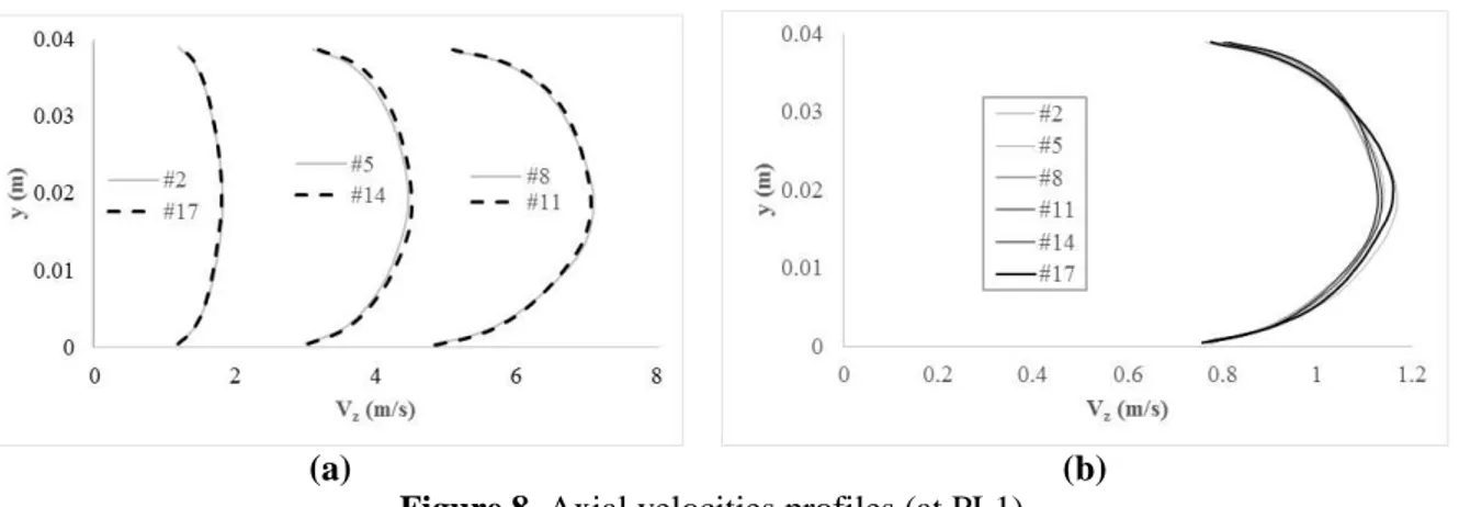
A very good repeatability of the results was observed as well as a good symmetry with respect to the axis. The various distributions of these flow velocity components, Vz, were divided by an average velocity Vq obtained by dividing the volume flow rate by the area of the cross section of the pipe and presented on figure 8, while on table 3 the PIV results are being compared with the reference flow rate.
(a) (b)
12
(a) (b)
Figure 8. Axial velocities profiles (at PL1)
Table 3. Comparison between PIV results and reference flow rates of the steady tests (at PL2) # QCF (m 3 /h) QPIV (m 3 /h) σ (m3/h) Vq (m/s) 2 7.14 6.93 0.216 1.51 5 17.98 17.55 0.468 3.80 8 28.77 28.21 0.720 6.08 11 28.75 28.17 0.792 6.08 14 18.03 17.66 0.468 3.81 17 7.21 7.07 0.216 1.52 20 18.04 17.62 0.504 3.81
On figure 9, an overall comparison between the reference flow rate and values measured by the US flowmeter, and the PIV method is being made. The PIV measurements were systematically underestimating the target flow rate, but with a relative difference always less than 2.5%, when compared with measurement from the CF, which can be considered satisfactory, taking into account, on the one hand, the lack of measurement points very close to the walls on the boundary layer, and, on the other hand, uncertainties in the flow velocity measurements with the PIV (principally links with calibration factors and localization of the PIV plane with respect to pipe diameter).
Figure 9. Mean flow rate from PIV (square) and ultrasonic flowmeter measurements (cross) compared
to the Coriolis flowmeter (at PL1) 4.2 The unsteady-state case
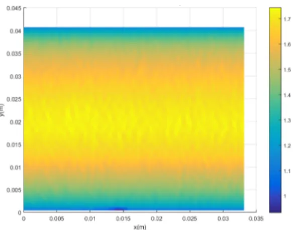
The results obtained from the PIV method and the PS have been used as references to be compared with the measurements of the US flowmeter. A characteristic PIV image is presented on figure 10. The post-processing consisted of:
• Determination, for each instantaneous velocity map, of a mean profile of velocities by averaging in the axial direction of the pipe.
13
• Integration of the instantaneous profile for calculating the instantaneous volume flow rate assuming that the flow is axi-symmetric.
• Calculation of the average volume flow rate over the total measurement period.
• Implementation of a Fourier transform on a set of instantaneous flow rate values.
• Determination of the amplitude of the flow rate fluctuations at the fundamental excitation frequency observed on the spectrum.
• Calculation of the average flow rate from FFT of the PIV images.
Figure 10. Distribution of the axial components of average velocities for Qnom = 7.2 m3/h & fnom = 8 Hz
From the Fourier analysis, it is possible to transform the PIV images into the frequency domain (figure 11). Then it was observed an emergence on the main excitation frequency and therefore a very good identification of the flow rate fluctuation. Also, the amplitudes of flow rate fluctuations do not depend on the position of the computation plane along the interrogation window, justifying the use of an average value over the whole window. However, some limitations, in terms of resolutions, in the detection of flow fluctuations were observed in “broadband” levels, which are being increased substantially with the average flow, hence with the Reynolds number of the mean flow.
Figure 11. Fourier analysis for Qnom = 7.2 m3/h & fnom = 8 Hz
In the case of the PS measurements, the application of the wave propagation model with a wave velocity considering the deformability of the pipe wall, made it possible to calculate the real and imaginary parts of the Fourier transform of the associated flow rate fluctuations; and thus, to access the amplitude of the flow fluctuations for each frequency value. Additionally, Fast Fourier transformations (denoted as FFT) were performed on the real and imaginary parts using custom build-in MATLAB routbuild-ines comparbuild-ing signals of two different sensors.
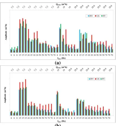
In a similar way, the same FFT algorithm was applied on continuous US unsteady measurements to determine the frequency and the amplitude of the flow rate fluctuations. On figure 12 all results of the flow fluctuations amplitudes at the fundamental frequency are being summarized and compared.
14
(a)
(b)
Figure 12. Comparison of the amplitude of flow fluctuations at the fundamental excitation frequency
obtained with the three methods at a) plane 1 and b) plane 2
In all flow tests the frequency of the imposed fluctuations has been perfectly identified by all methods. However, it seems that in the case of the US the "background noise" increases with the Reynolds number. Consequently, at high flow rates the detection of fluctuations with smaller amplitudes becomes less evident. The diminution of the amplitude of the fluctuation with the dominant frequency of excitation was observed with all methods and was clearly attributed to the experimental way of creating the disturbances on the flow.
Almost systematically, the amplitudes of flow fluctuations obtained with the US flowmeter are greater than those obtained with the PIV and the PS. These differences can probably be attributed to : i/ the use of data signals coming from two measuring lines located in the two different US flowmeters bodies. During unsteady operations, the propagating time of perturbations between the two bodies are not taken into account in the present work. It can be remembered that the use of two bodies was chosen in order to prevent signal interferences between the two lines. ii/ the use of a calibration constants coming from steady operating conditions. Also, between the PIV and the PS results there was a difference that can be probably attributed to some limitations of the model used for the post-treatment of pressure fluctuations.
5. Conclusions
An ultrasonic flowmeter consisting of two bodies has been developed for further applications in cryogenic conditions and for measuring flow rate fluctuations in the range of 0 to 70 Hz. A calibration procedure has been successfully established for water flows in a pipe using a Coriolis flowmeter as reference and the acquired transit times of at least two measurements lines of the developed US flowmeter. During steady state flow tests the average difference between the US and the reference method was better than 5% when lines belonging on different bodies were paired.
15 Flow velocity measurements in a transparent section installed immediately downstream of the ultrasonic flowmeter have been performed using high speed particle image velocimetry in two planes. Tests in steady operating conditions using again the Coriolis flowmeter as reference validated the method of obtaining the volume flow rate by integrating the axial components of flow velocities. The PIV values were always below the reference values with less than 2.5% of relative difference, permitting the implementation of the method as a reference in the studies of unsteady flows.
Additionally, recordings of three pressure sensors flush mounted on the pipe wall upstream of the US flowmeter were systematically performed during unsteady tests, in order to apply a well-known hydro-acoustics model and to measure the frequency and amplitude of the imposed fluctuations on the flow. The Fourier transformations of the signals originating from the US flowmeter clearly showed the capability of the method to fully identify the excitation frequencies, including the higher excitation frequencies tested (70 Hz) for which the fluctuation levels were weak. Concerning the amplitude of the imposed disturbances, the values obtained with the US flowmeter differ from the measurements obtained with the other two methods (with a maximum relative error of around 2%) overestimating the amplitude. The main challenges for improving the accuracy of the measurements methods are the following :
- Find a way to minimize the effects of the interferences between measuring lines,
- The development of a new method for the generation of the flow rate fluctuation with a better signal to noise ratio. This new device could be used for a direct unsteady calibration procedure.
References
[1] Sieverding C, Arts T, Denos R and Brouckaert J 2000 Measurement techniques for unsteady flows in turbomachines Exp. Fluids 28 285-321
[2] Hogendoorn J, Boer A and Danen H 2007 An ultrasonic flowmeter for custody transfer measurement of LNG: A challenge for design and calibration 25th Int. North Sea Flow Measurement Workshop Oslo
[3] Grenier P 1991 Effects of unsteady phenomena on flow metering Flow Meas. Instrum. 2 74-80 [4] Mattingly GE and Yeh TT 1991 Effects of pipe elbows and tube bundles on selected types of
flowmeters Flow Meas. Instrum. 2 4-13
[5] Cheesewright R, Clark C and Bisset D 2000 The identification of external factors which influence the calibration of Coriolis mass flowmeters Flow Meas. Instrum. 11 1-10
[6] Berrebi J, Martinsson PE, Willatzen M and Delsing J 2004 Ultrasonic flow metering errors due to pulsating flow Flow Meas. Instrum. 15 179-85
[7] Bobovnik G, Kutin J, Mole N, Stok B and Bajsić I 2013 Numerical analysis of installation effects in Coriolis flowmeters: A case study of a short straight tube full-bore design Flow Meas. Instrum. 34 142-50
[8] Bates J 2000 Performance of two electromagnetic flowmeters mounted downstream of a 90° mitre bend/reducer combination Measurement 27 197-206
[9] Heritage JE 1989 The performance of transit time ultrasonic flowmeters under good and disturbed flow conditions Flow Meas. Instrum. 1 24-30
[10] Halttunen J 1990 Installation effects on ultrasonic and electromagnetic flowmeters: A model-based approach Flow Meas. Instrum. 1 287-92
[11] Furness RA 1991 BS7405: The principles of flowmeter selection Flow Meas. Instrum. 2 233-42 [12] Mottram R 1992 Introduction: An overview of pulsating flow measurement Flow Meas.
Instrum. 3 114-7
[13] Vetter G and Notzon S 1994 Effect of pulsating flow on Coriolis mass flowmeters Flow Meas. Instrum. 5 263-73
16 [14] Cheesewright R, Clark C and Hou YY 2004 The response of Coriolis flowmeters to pulsating
flows Flow Meas. Instrum. 15 59-67
[15] Hebrard P, Malard L and Strzelecki A 1992 Experimental study of a vortex flowmeter in pulsatile flow conditions Flow Meas. Instrum. 3 173-86
[16] Laurantzon F, Örlü R, Segalini A and Alfredsson PH 2010 Time-resolved measurements with a vortex flowmeter in a pulsating turbulent flow using wavelet analysis Meas. Sci. Technol. 21 123001
[17] Hakansson E and Delsing J 1994 Effects of pulsating flow on an ultrasonic gas flowmeter Flow Meas. Instrum. 5 93-101
[18] Doblhoff-Dier K, Kudlaty K and Wiesinger M 2010 Time resolved measurement of pulsating flow using orifices Flow Meas. Instrum. 22 97-103
[19] Beaulieu A, Foucault E, Braud P, Micheau P and Szeger P 2011 A flowmeter for unsteady liquid flow measurements Flow Meas. Instrum. 22 131-7
[20] Nabavi M and Siddiqui K 2010 A critical review on advanced velocity measurement techniques in pulsating flows Meas. Sci. Technol. 21 042002
[21] Laurantzon F, Tillmark N, Örlü R and Alfredsson PH 2012 A flow facility for the characterization of pulsatile flows Flow Meas. Instrum. 26 10-7
[22] Tanaka T and Tsukamoto H 1999 Transient behavior of a cavitating centrifugal pump at rapid change in operating conditions—Part 2: Transient phenomena at pump startup/shutdown J. Fluids Eng. 121 850-6
[23] Dazin A, Caignaert G and Bois G 2007 Transient behavior of turbomachineries: Applications to radial flow pump startups J. Fluids Eng. 129 1436-44
[24] Rubin S 1966 Longitudinal instability of liquid rockets due to propulsion feedback (Pogo) J. Spacecr. Rockets 3 1188-95
[25] Brennen CE. 1994 Hydrodynamics of Pumps Concepts ETI, Inc & Oxford University Press [26] Yamamoto K, Müller A, Ashida T, Yonezawa K, Avellan F and Tsujimoto Y 2015
Experimental method for the evaluation of the dynamic transfer matrix using pressure transducers J. Hydraulic. Research 52 66-77
[27] Carta F, Bolpaire S, Charley J and Caignaert G 2002 Hydroacoustics source characterization of centrifugal pumps Int. J. Acoust. Vib. 7 110-4
[28] Lauro JF and Boyer A 1998 Matrice de transfert et sources hydrodynamiques d'une pompe centrifuge à faibles charges La Houille Blanche 3/4 128-33
[29] Lefebvre PJ and Durgin WW 1990 A transient electromagnetic flowmeter and calibration facility J. Fluids Eng. 112 12-15
[30] Lynnworth LC and Liu Y 2006 Ultrasonic flowmeters: Half-century progress report, 1955-2005 Ultrasonics 44 1371-8
[31] Coman IM and Popescu BA 2015 Shigeo Satomura: 60 years of Doppler ultrasound in medicine Cardiovasc. Ultrasound 13 48-50
[32] Kaneko Z 1986 First steps in the development of the Doppler flowmeter Ultrasound Med. Biol.
12 187-95
[33] Takeda Y 1995 Velocity profile measurement by ultrasonic Doppler method Exp. Thermal Fluid Sci. 10 444-53
[34] Coulthard J 1973 Ultrasonic cross-correlation flowmeters Ultrasonics 11 83-8
[35] Mori M, Takeda Y, Taishi T, Furuichi N, Aritomi M and Kikura H 2002 Development of a novel flow metering system using ultrasonic velocity profile measurement Exp. Fluids 32 153-60
[36] Wada S, Kikura H, Aritomi M, Mori M and Takeda Y 2004 Development of pulse ultrasonic Doppler method for flow rate measurement in power plant. Multilines flow rate measurement on metal pipe J. Nucl. Sci. Techn. 41 339-46
[37] Renard D, Gasnier J and Guillon A 1987 Vélocimétrie et débitmétrie: méthodes basées sur les ultrasons La Houille Blanche 4/5 305-12
17 [38] Chen Q, Li W and Wu J 2014 Realization of a multipath ultrasonic gas flowmeter based on
transit-time technique Ultrasonics 54 285-90
[39] Cousins T and Augenstein D 2002 Proving of multi-path liquid ultrasonic flowmeters 20th Int. North Sea Flow Measurement Workshop Glasgow
[40] Iooss B, Lhuillier C and Jeanneau H 2002 Numerical simulation of transit-time ultrasonic flowmeters: uncertainties due to flow profile and fluid turbulence Ultrasonics 15 179-85
[41] Ma L, Liu J and Wang J 2012 Study of the accuracy of ultrasonic flowmeters for liquid AASRI Procedia 3 14-20
[42] Bobovnik G, Kutin J and Bajsić I 2004 The effect of flow conditions on the sensitivity of the Coriolis flowmeter Flow Meas. Instrum. 15 69-76
[43] Hogendoorn J, Hofstede H, van Brakel P and Boer A 2011 How accurate are ultrasonic flowmeters in practical conditions; Beyond the calibration 29th Int. North Sea Flow Measurement Workshop Tonsberg
[44] Raffel M, Willert C, Wereley S and Kompenhans J 2007 Particle Image Velocimetry - A practical guide Springer
[45] Soria J 1996 An investigation of the near wake of a circular cylinder using a video-based digital cross-correlation particle image velocimetry technique Exp. Therm. Fluid Sci. 12 221-33
[46] Willert C and Gharib M 1991 Digital particle image velocimetry Exp. Fluids 10 181-93 [47] Scarano F 2002 Iterative image deformation methods in PIV Meas. Sci. Technol. 13 1-19 [48] Lecordier B and Trinité M 2004 Advanced PIV algorithms with image distortion validation and
comparison using synthetic images of turbulent flow EUROPIV 2 Workshop: Particle Image Velocimetry: Recent Improvements Zaragoza