A Novel Approach for Simplification of Industrial Robot Dynamic Model Using Interval Method

Science Arts & Métiers (SAM)

is an open access repository that collects the work of Arts et Métiers Institute of

Technology researchers and makes it freely available over the web where possible.

This is an author-deposited version published in: https://sam.ensam.eu

Handle ID: .http://hdl.handle.net/10985/8754

To cite this version :

Ke WANG, François LEONARD, Gabriel ABBA - A Novel Approach for Simplification of Industrial Robot Dynamic Model Using Interval Method - In: IEEE/ASME International Conference on Advanced Intelligent Mechatronics, AIM 2014, France, 2014-07-08 - Proceedings of IEEE/ASME International Conference on Advanced Intelligent Mechatronics - 2014

Any correspondence concerning this service should be sent to the repository Administrator : archiveouverte@ensam.eu

A Novel Approach for Simplification of Industrial Robot Dynamic

Model Using Interval Method*

Ke Wang

, Franc¸ois L´eonard

and Gabriel Abba

, Member, IEEE

Abstract— This paper proposes a new approach to simplify

the dynamic model of industrial robot by means of interval method. Due to strong nonlinearities, some components of robot dynamic model such as the inertia matrix and the vector of centrifugal, Coriolis and gravitational torques, are very complicated for real-time control of industrial robots. Thus, a simplification algorithm is presented in this study in order to reduce the computation time and memory occupation. More importantly, this simplification is suitable for arbitrary tra-jectories in whole robot workspace. Furthermore, the method devotes to finding negligible inertia parameters, which is useful for robot model identification. A simulation has been carried out on a test trajectory using a 6-DOF industrial robot model, and the results have shown good performance and effectiveness of this method.

I. INTRODUCTION

Robot manipulators have been increasingly used in various industrial applications in recent years, such as assembly, spray painting, materials machining and welding tasks, im-proving the productivity, flexibility, and quality. However, for most industrial robots applied to machining and Friction Stir Welding (FSW) process, a high precision and real-time performance can not be achieved. In order to ensure a better tracking performance, many studies about industrial robot control have been performed. Although the machining accuracy can be raised by means of observer-based control or other methods [1], it can not avoid to bring a more complicated control structure. As a result, a great deal of calculation and memory occupation will be carried out in robot controller, affecting the real-time capability. Therefore, low complexity models are essential and model reduction methods are very useful tools.

Industrial manipulators are highly nonlinear, highly cou-pled and time-varying systems. There exist many model re-duction methods available for nonlinear systems [2], includ-ing heuristic methods, linearization around equilibrium point or trajectory, balancing using energy functions, balancing empirical Gramians [3], proper orthogonal decomposition, trajectory piecewise-linear approach [4], model reduction through system identification. A computationally efficient

*This work was sponsored by the French National Agency of Research under the project ANR-2010-SEGI-003-01-COROUSSO, and China Schol-arship Council (CSC, File No. 201206020028). The authors would like to thank J. Qin and M. Zouhri for their support.

1_{Ke Wang is with Laboratoire de Conception, Fabrication et Commande}

(LCFC), Arts et M´etiers ParisTech, 4 rue Augustin Fresnel, 57078 Metz Cedex 3, France (E-mail: ke.wang@ensam.eu).

2_{Franc¸ois L´eonard and Gabriel Abba are with Laboratoire de}

Concep-tion, Fabrication et Commande (LCFC), Ecole Nationale d’Ing´enieurs de Metz, 1 route d’Ars Laquenexy, 57078 Metz Cedex 3, France (E-mail: leonard@enim.fr, gabriel.abba@ensam.eu).

reduction method relating to balanced truncation was also proposed in [5]. All these methods can reduce the number of states and improve calculation speed, while the limitation is that they are only applicable to specific trajectories.

Interval method has been widely used in various applica-tions [6], [7], such as parameter and state estimation, robust control and robotics, etc. Using interval analysis, Kieffer and Jaulin [8] proposed a guaranteed recursive nonlinear state estimator, which can solve many actual tracking problems. Its applications to the robust autonomous localization and tracking of mobile robots were presented in [9], [10]. The main limitation of such technique lies in the explosion of complexity with the number of state variables. A similar robust navigation method was also applied to sailboat robots [11], and an interval-based method for the validation of reliable and robust navigation rules was given meanwhile. The authors of [12] combined the interval computation and constraint propagation to tackle some difficult problems in nonlinear identification and robust control.

In the field of industrial robots, a new approach based on interval analysis was developed to find the global minimum-jerk (MJ) trajectory of a robot manipulator within a joint space scheme using cubic splines [13]. The geometric design issue of serial-link robot manipulators with three revolute (R) joints was solved for the first time using an interval analysis method [14]. Gouttefarde et al. [15] presented an interval-analysis-based approach to the wrench-feasible workspace determination of n-DOF parallel robots driven by n or more cables. In [16], a novel approach based on interval method was used to deal with problems of dynamic self-collision detection and prevention for 2-DOF robot manipulator. The forward kinematic map of serial manipulator was extended to intervals using the product of exponential formulation in order to analyze the kinematic errors [17].

As for model simplification using interval method, Martini proposed a method to simplify a 7-DOF helicopter model [18]. During this simplification, the terms related to the com-ponents of the inertia matrix and the vector of centrifugal, Coriolis and gravitational torques were first studied from the point of view of specific trajectories, including the normal and helical trajectories. Then all the terms were analyzed by using interval method, which could be generalized to arbitrary trajectories. A simulation for the two trajectories was carried out to demonstrate effectiveness of this method as well. Nevertheless, his method is limited to some specific flight trajectories.

The objective of this paper is to propose a simplification approach for the dynamic model of heavy industrial

ma-nipulator using interval method. In the model-based control design, simple models are highly preferred. By applying the resulting simplified model to practical control system, the computation time and memory occupation will be greatly reduced, particularly in the observer-based control presented by Qin et al. [1], [19]–[21]. What is more important is that this simplification is suitable for arbitrary trajectories in whole robot workspace. Moreover, the simplification devotes to finding negligible inertia parameters, which is very useful for robot model identification.

This paper is organized as follows: The modeling of an in-dustrial manipulator KUKA KR500-2MT is firstly presented in Section II. In Section III the definition and operation of interval is introduced, followed by the simplification algorithm of robot model and results for whole workspace. In Section IV, a simulation is carried out on a test trajectory to verify the performance of simplification. Section V provides some usage of the simplified model. Finally, Section VI concludes this paper by discussing the advantage of this simplification.

II. ROBOTDYNAMICMODEL

The industrial robot considered in this study is a serial manipulator KUKA KR500-2MT, as shown in Fig. 1. It has six degrees of freedom, and is composed of six moving links and six revolute joints. We would like to use this robot model to present our simplification method. In order to simplify the modeling of robot, we assume that the tool is directly fixed on link 6 and the spindle of tool is coincident with the axis of joint 6.

Fig. 1. Robot KUKA KR500-2MT (by courtesy of Institut de Soudure)

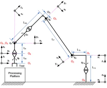
On the basis of the research work of Khalil and Dombre [22], the modified Denavit-Hartenberg geometric description is commonly adopted in the modeling of robots. Fig. 2 shows a geometric description of the robot manipulator. After defin-ing the reference frames for the robot, the Modified Denavit-Hartenberg notation can be applied to obtain the geometric parameters, which are listed in Table I. The numerical values of these parameters used for the simplification are given in Table VI of Appendix.

In accordance with this description, the robot motion can be completely described by the vector q of six generalized coordinates: q = [q1, q2, q3, q4, q5, q6]T. The description

fa-cilitates to calculate symbolic expressions of the geometric,

Fig. 2. Geometric description of the robot [1] TABLE I

GEOMETRICPARAMETERS OFROBOTMODEL[1]

j µj σj αj dj θj rj 1 1 0 π 0 q1 −L1z 2 1 0 π/2 L1x q2 0 3 1 0 0 L2 π/2 + q3 0 4 1 0 −π/2 −D4 q4 −L34 5 1 0 π/2 0 q5 0 6 1 0 −π/2 0 −π/2 + q6 −L5 t 0 2 0 0 0 −Ltz

kinematic and dynamic model of robot with the help of the software SY MORO+ [23], [24], or other robotic techniques. Using the Newton-Euler method or the Lagrange equa-tions, one can get the dynamic model of the robot as the following form [1]:

M(q) ¨q + H(q, ˙q) + Ff r( ˙q) + JT(q)F =Γ (1) where M(q)(6×6) is the symmetric, uniformly positive

def-inite and bounded inertia matrix, H(q, ˙q)(6×1) represents

the vector of centrifugal, Coriolis and gravitational torques,

Ff r( ˙q)(6×1) is the vector of friction at the robot axis, F(6×1)

is the vector of efforts applied by robot on external envi-ronment, JT(q)_(6×6) is the transposed Jacobian matrix of the tool frame, Γ_(6×1) is the vector of gearbox torque, and q,

˙

q and ¨q represent the robot angular position, velocity and

acceleration vectors respectively.

III. SIMPLIFICATIONUSINGINTERVALMETHOD

A. Basic Definitions and Operations of Intervals

The interval denoted by [a, b] is the closed set of real numbers given by:

[a, b] ={x ∈ R : a ≤ x ≤ b} (2)

If the left and right endpoints of an interval X are denoted by X and X respectively, the width, midpoint and

absolute value of this interval X can be defined as follows:

m(X ) = (X + X )/2 (4)

|X| = max{|X|,|X|} (5) Let X , Y be real compact intervals and the general form of the interval arithmetic operations are defined as:

X⊙Y = {x ⊙ y : x ∈ X,y ∈ Y} (6) where ⊙ stands for one of the basic operations including addition, subtraction, multiplication and division, and here we assume 0 /∈ Y in case of division. In addition, these operations can be expressed in terms of the endpoints of intervals, and the following rules hold:

X +Y = [X +Y , X +Y ] (7) X−Y = [X −Y,Y − X] (8) X·Y = [min{XY,XY,XY,XY},max{XY,XY,XY,XY}] (9) X /Y = X·1 Y, where 1 Y = [1/Y , 1/Y ] i f 0 /∈ Y (10)

Similarly the notion of intervals and interval arithmetic can be extended to include interval vectors and interval matrices as well. More details about intervals are presented in the books of Moore [6] and Jaulin [7].

B. Simplification Algorithm

From (1), we can observe that the expressions of some components are very complicated, such as the inertia matrix

M(q) and the vector of centrifugal, Coriolis and gravitational

torques H(q, ˙q). All expressions of these components show

strong nonlinearities and a high coupling between the control inputs, which make it difficult to design the control law of robot. Therefore, it is necessary to simplify these expressions in order to acquire a simple model containing essential terms and characteristics of the robot manipulator.

Various model reduction methods for nonlinear systems are existent, however, most of them are only applicable to specific trajectories. According to the specification of robot KUKA KR500-2MT, the range of angular motion, velocity and acceleration for each axis are given in Table II. As shown in this table, all the variables about trajectories in operational workspace are intervals. As a result, interval method will be an easier and more effective way to simplify robot dynamic model compared with other methods. More importantly, the interval-method-based simplification can be definitely applied to arbitrary trajectories in robot workspace.

TABLE II

RANGE OFROBOTMOTION, VELOCITY ANDACCELERATION

Axis Angular Motion Velocity Acceleration 1 ±185◦ ±42◦/s ±59◦/s2 2 −130◦to + 20◦ ±42◦/s ±43◦/s2 3 −94◦to + 150◦ ±42◦/s ±78◦/s2 4 ±350◦ ±76◦/s ±42◦/s2 5 ±118◦ ±74◦/s ±92◦/s2 6 ±350◦ ±123◦/s ±68◦/s2

For every component of inertia matrix M(q)(6×6) and

vector H(q, ˙q)_(6×1) in (1), its expression can be described as follows:

Mi j= f1(sin(qm), cos(qn))

Hi= f2(sin(qm), cos(qn), ˙ql)

(11)

where i, j, m, n, l∈ {1,2,3,4,5,6}, f1and f2are maps. Thus,

a simple component can be taken as an instance to address the simplification algorithm, such as M44, formulated as:

M44= ZZ4R+ ZZ6c25+ 2XY5c5s5+ 2L5MY6c5c6s5

+ 2Y Z6c5c6s5+ X X5Rs25+ 2L5MX6c5s5s6

+ 2X Z6c5s5s6+ 2XY6c6s25s6+ X X6Rs25s26

(12)

where si, ci denote sin(qi) and cos(qi) respectively, ZZ4R,

ZZ6, XY5, MY6, Y Z6, X X5R, MX6, X Z6, XY6, and X X6Rare 10

of 36 regrouped inertia parameters used in robot modeling, and more details can be found in [20], [25]. The whole algorithm process can be divided into 3 steps.

1) Compress the interval

First of all, some trigonometric transformations can be used to rewrite products and powers of sine and cosine func-tions in the expression, in terms of trigonometric funcfunc-tions with combined arguments. For example:

2 cos2(x) = 1 + cos(2x)

2 sin(x) cos(y) = sin(x + y) + sin(x− y) (13) Then we carry out the following transformation:

a cos(x) + b sin(x) =√a2_{+ b}2_{cos(x− arctan(a,b)) (14)}

Accordingly the component M44 is transformed as:

M₄₄′ = 10

∑

4t0cos(2q6− arctan(−XX6R, 2XY6)) +1

8t0cos(2q5+ 2q6− arctan(XX6R,−2XY6)) +1

8t0cos(2q5− 2q6− arctan(XX6R, 2XY6)) +1 2 √ t₁2+ t₂2cos(2q5+ q6− arctan(−t1,t2)) +1 2 √ t₁2+ t₂2cos(2q5− q6− arctan(t1,t2)) +1 4 √ t₃2+ t2 4cos(2q5− arctan(t3,t4)) (15) where t0= √ X X_6R2 + 4XY₆2, t1= L5MX6+X Z6, t2= L5MY6+

Y Z6, t3= 2ZZ6− 2XX5R− XX6R, t4= 4XY5. As a result, the

number of terms in the component is reduced from 16 to 10, and the interval is compressed from [−8.8580,306.27] to [76.007, 195.34] without any approximation.

2) Remove unimportant terms

The norm of an interval, also called absolute value, can be gained from (5). Since most of terms in the expression are intervals, it is possible to compare them by calculating their norms. Define kt as a proportional factor, then any term Ti can be neglected if it satisfies:

|Ti|

g(|T1|, |T2|, ··· , |Tn|)≤ k

t (16)

where n is total number of terms of a component, g is one of maps which can find the maximum value, sum and root mean square (RMS) value of inputs. In this paper, the maximum value map is adopted. This step can be illustrated by M₄₄′ in (15), and the norm ratio of each term to maximum one is provided in Table III, except the first 4 constant terms.

TABLE III

NORMRATIO OFEACHTERM TOMAXIMUM

Term T5 T6 T7 T8 T9 T10

Ratio(%) 33.6 16.8 16.8 2.30 2.30 100

If kt is chosen as 5%, correspondingly the term T8and T9

in expression (15) will be removed. The simplified compo-nent is in the range of [77.611, 193.74], approximately equal to the original one.

3) Neglect unimportant inertia parameters

As a matter of fact, not every inertia parameter has a great influence on norm of a term. Take the term T10 in (15) for

an instance, the inertia parameter X X5R, XY5, X X6R, and ZZ6

are found in the expression. Define kpas a new proportional factor, then any inertia parameter P can be removed if it meets the following condition:

ep=| |T|P=0_|T|− |T| |≤ kp (17) The result is given in Table IV. Assuming that kpis assigned to 15%, the inertia parameter XY5 can be neglected.

TABLE IV

NORM OFTERM ANDERROR ASP=0

P none X X5R XY5 X X6R ZZ6

Norm 34.727 27.726 30.225 26.390 25.211

ep(%) 0 20.16 12.96 24.01 27.40

C. Programming and Results

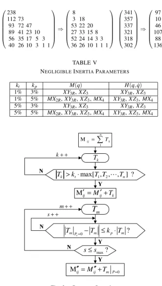
In the light of above algorithm, programs are developed by using Mathematica well-known for symbolic and interval calculations. The flow chart of the program can be seen in Fig. 3. The results are valid for the whole workspace. Choosing kt= 5% and kp= 5%, the change in the number of terms and negligible inertia parameters for M(q) and H(q, ˙q)

are respectively listed below:

       238 112 73 93 72 47 89 41 23 10 56 35 17 5 3 40 26 10 3 1 1       ⇒        8 3 18 53 22 20 27 33 15 8 52 24 14 3 3 36 26 10 1 1 1               341 357 337 321 318 302       ⇒        97 10 46 107 88 136        TABLE V

NEGLIGIBLEINERTIAPARAMETERS

kt kp M(q) H(q, ˙q) 1% 3% XY3R, X Z3 XY3R, X Z3 1% 5% MX2R, XY3R, X Z3, MX4 XY3R, X Z3, MX4 5% 3% XY3R, X Z3 XY3R, X Z3 5% 5% MX2R, XY3R, X Z3, MX4 XY3R, X Z3, MX4 1 M n ij=

∑

T

Fig. 3. Program flow chart

IV. SIMULATION ON A TESTTRAJECTORY

A simulation is carried out on a test trajectory (see Fig. 4), in order to analyze the effectiveness and performance of the simplification method. According to the trajectory data, the interval of angular position, velocity and acceleration can be found in Table VII of Appendix.

Generally, the proportional factors kt and kp can be se-lected intuitively. Calculating the root mean square (RMS) errors can also be considered as a good approach. In this case, three representative components are chosen to find the most appropriate factors, including M11, M21, and M22. Based

on the balance between accuracy and simplicity, the number of terms after simplification, RMS error, and value range of component are taken into account.

As a result, we select kt= 3%, and kp= 1%. The change in the number of terms for each component of inertia matrix

M(q) and the corresponding RMS errors are shown as:

       238 112 73 93 72 47 89 41 23 10 56 35 17 5 3 40 26 10 3 1 1       ⇒        14 12 26 61 39 24 27 37 19 8 52 32 14 3 3 40 26 10 3 1 1       

0 5 10 15 −3 −2 −1 0 1 2 Time [s]

Angular Position [rad]

0 5 10 15 −1 −0.5 0 0.5 1 1.5 Time [s]

Angular Velocity [rad/s]

0 5 10 15 −4 −3 −2 −1 0 1 2 3 Time [s]

Angular Acceleration [rad/s

2] 0 1000 2000 −1000 0 1000 2000 3000 1500 2000 2500 3000 X [mm] Y [mm] Z [mm] motion trajectory starting point

axis 1 axis 2 axis 3 axis 4 axis 5 axis 6

Fig. 4. Angular position and velocity in the trajectory of FSW

eRMS(%) =        1.08 4.46 0.77 3.07 2.48 0.83 9.68 1.57 0.55 0.38 0.91 1.60 1.56 1.29 0 3.64 0 0 0 0 0       

Similarly, by choosing kt= 3%, and kp= 1%, the change in the number of terms for each component of vector H(q, ˙q)

and the corresponding RMS errors are given as follows:

       341 357 337 321 318 302       ⇒        147 46 66 153 116 170        eRMS(%) =        5.89 4.41 4.11 8.38 4.99 2.83       

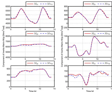
Fig. 5 and Fig. 6 show the comparison between simplified and original component for M(q) and H(q, ˙q). From these

figures, it can be seen that on the whole the simplified model is in good agreement with original one, even though some components may not match exactly, such as M41.

However, it should be mentioned that all of the inertia parameters, which are obtained through model identification, have a certain degree of error [20]. Compared with the accu-racy of inertia parameter, the error caused by simplification in this simulation is acceptable, and the global RMS errors of M(q) and H(q, ˙q) are 0.95% and 4.41% respectively.

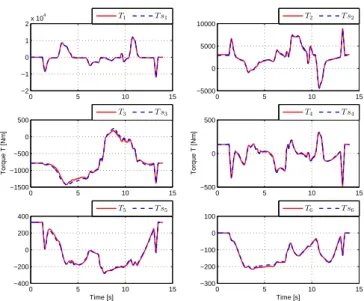
In fact, the torque T = M(q) ¨q + H(q, ˙q) in (1) is frequently

computed in practical control. Fig. 7 gives the comparison between simplified and original component of torque T , and the RMS errors for each axis are 1.07%, 3.44%, 4.07%, 7.5%, 5.6%, and 2.77% respectively. Furthermore, the global RMS error of torque T is 2.61%. All the above simulation results shows a good performance of simplification.

V. DISCUSSION ONUSAGE OFSIMPLIFIEDMODEL

Seen from the simulation results, the simplified model is much simpler than the original one while with enough accuracy. As a consequence, the simplified model can be

0 5 10 15 3500 4000 4500 5000 5500 6000 0 5 10 15 −200 0 200 400 600 800 0 5 10 15 4000 5000 6000 7000 8000

Component of Inertia Matrix M(q) [Nms

2/rad] 0 5 10 15 −50 0 50 100

Component of Inertia Matrix M(q) [Nms

2/rad] 0 5 10 15 0 200 400 600 Time [s] 0 5 10 15 0 50 100 150 200 Time [s] M11 M s11 M21 M s21 M22 M s22 M31 M s31 M32 M s32 M41 M s41

Fig. 5. Comparison between simplified and original component in M(q)

0 5 10 15 −800 −600 −400 −200 0 200 0 5 10 15 0 1000 2000 3000 4000 0 5 10 15 −1500 −1000 −500 0 500

Component of Vector H of Centrifugal, Coriolis and Gravitational Torques [Nm]

0 5 10 15 −300 −200 −100 0 100 200

Component of Vector H of Centrifugal, Coriolis and Gravitational Torques [Nm]

0 5 10 15 −400 −200 0 200 400 Time [s] 0 5 10 15 −200 −100 0 Time [s] H1 H s1 H2 H s2 H3 H s3 H4 H s4 H5 H s5 H6 H s6

Fig. 6. Comparison between simplified and original component in H(q, ˙q)

applied to many control methods to simplify the control structure and improve the real-time performance, such as the computed torque controller or the observer-based control.

In the research work presented by Qin et al. [1], [19]– [21], as a strong external force is exerted on the robot during the machining or FSW process, the natural stiffness of industrial robot is not sufficient. To compensate the manipulator deformation, a nonlinear observer is designed to estimate the robot states (q, ˙q, ¨q) and the external force F.

In this observer-based control for robot KUKA KR500-2MT, a corrected target position is given to the interpolator of robot controller every 12ms so as to compensate the error between the desired position and so-called real position esti-mated by a discrete observer, whose sampling time is 1.2ms [21]. The diagram of external deformation compensation of KUKA robot is provided in Fig. 8, which can explain the

0 5 10 15 −2 −1 0 1 2x 10 4 T1 T s1 0 5 10 15 −5000 0 5000 10000 T2 T s2 0 5 10 15 −1500 −1000 −500 0 500 Torque T [Nm] T3 T s3 0 5 10 15 −500 0 500 Torque T [Nm] T4 T s4 0 5 10 15 −400 −200 0 200 400 Time [s] T5 T s5 0 5 10 15 −300 −200 −100 0 100 Time [s] T6 T s6

Fig. 7. Comparison between simplified and original torque T

reason why the simplification is needed for this control.

Controller of KUKA (sampling time: 12ms) target position + + Trajectory

interpolator RobotKUKA

torque reference sensors values Discrete observer (sampling time: 2ms) motor position current position correction

Fig. 8. External deformation compensation of KUKA robot [21]

With regard to the estimation of external force in the above observer-based control, it can be obtained by:

b

F =−J−T(q)M(q)zb4 (18)

where bF denotes estimated external force, and zb4 denotes

observer state 4 [1]. Obviously, the inertia matrix M(q) can be replaced by the simplified one Ms(q) in (18).

In addition, the resulting negligible inertia parameters have a significant meaning for the robot model identification. The identified inertia parameters will be more precise as the negligible inertia parameters are removed [25].

VI. CONCLUSIONS

A new approach using interval method for simplification of industrial robot dynamic model is presented in this paper. From the symbolic dynamic model of a 6-DOF industrial manipulator, all the expressions of components in inertia matrix M(q) and vector H(q, ˙q) show complexities and

strong nonlinearities, besides, a high coupling between con-trol inputs also exists. Thus, a simplification algorithm is proposed to make the robot model much simpler. As a simple component of inertia matrix, M44is taken to illustrate

the entire process. The results for the whole workspace are suitable for arbitrary trajectories. A simulation on a test trajectory is carried out and the comparisons between simplified and original components of M(q), H(q, ˙q) and

T are performed. A good accuracy of the simplified model

is shown, demonstrating the effectiveness and good perfor-mance of the method. The simplified model can be applied to the observer-based control, and it also devotes to finding negligible inertia parameters, which is very useful for robot model identification.

APPENDIX

TABLE VI

NUMERICALVALUES OFROBOTGEOMETRICPARAMETERS

Length L1x L1z L2 L34 D4 L5 Ltz

(m) 0.500 1.045 1.300 1.025 0.055 0.235 0.435

TABLE VII

ACTUALINTERVAL OF THEANGULARPOSITION ANDVELOCITY

Axis AngularPosition(rad) Velocity(rad/s) Velocity(rad/s2) 1 [-1.3457,0.6393] [-0.7091,0.7141] [-2.5811,2.2603] 2 [-1.9929,-0.9411] [-0.2951,0.5056] [-1.4035,1.2476] 3 [-0.1359,1.5707] [-0.6485,0.7263] [-3.0617,1.6341] 4 [-0.8298,0.5699] [-0.9569,0.6014] [-1.3964,1.2582] 5 [-0.5254,1.5709] [-0.7805,1.3723] [-1.9199,1.6932] 6 [-2.4747,0] [-0.7331,0.9391] [-3.9371,1.5219] REFERENCES

[1] J. Qin, F. L´eonard, and G. Abba, “Experimental external force esti-mation using a non-linear observer for 6 axes flexible-joint industrial manipulators,” in The 9th Asian Control Conference, ASCC 2013, Istanbul, Turkey, June 2013, pp. 701–706.

[2] O. Nilsson, “On modeling and nonlinear model reduction in auto-motive systems,” Ph.D. dissertation, Lund University, Lund, Sweden, 2009.

[3] S. Lall, J. Marsden, and S. Glavaˇski, “A subspace approach to balanced truncation for model reduction of nonlinear control systems,”

International Journal of Robust and Nonlinear Control, vol. 12, no. 6,

pp. 519–535, 2002.

[4] D. Vasilyev, M. Rewie´nski, and J. White, “Macromodel generation for biomems components using a stabilized balanced truncation plus tra-jectory piecewise-linear approach,” IEEE Transactions on

Computer-Aided Design of Integrated Circuits and Systems, vol. 25, no. 2, pp.

285–293, 2006.

[5] O. Nilsson and A. Rantzer, “A novel nonlinear model reduction method applied to automotive controller software,” in Proceedings of the

American Control Conference, 2009, pp. 4587–4592.

[6] R. Moore, R. Kearfott, and M. Cloud, Introduction to Interval Analysis. Philadelphia, PA, USA: SIAM, 2009.

[7] L. Jaulin, Applied Interval Analysis: With Examples in Parameter and

State Estimation, Robust Control and Robotics. London: Springer, 2001.

[8] M. Kieffer, L. Jaulin, and E. Walter, “Guaranteed recursive nonlinear state estimation using interval analysis,” in Proceedings of the IEEE

Conference on Decision and Control, vol. 4, 1998, pp. 3966–3971.

[9] M. Kieffer, L. Jaulin, E. Walter, D. Meizel, et al., “Guaranteed mobile robot tracking using interval analysis,” in Proceedings of MISC’99,

Workshop on Application of Interval Analysis to System and Control,

1999, pp. 347–360.

[10] M. Kieffer, L. Jaulin, . Walter, and D. Meizel, “Robust autonomous robot localization using interval analysis,” Reliable Computing, vol. 6, no. 3, pp. 337–362, 2000.

[11] L. Jaulin and F. Le Bars, “An interval approach for stability analysis: Application to sailboat robotics,” IEEE Transactions on Robotics, vol. 29, no. 1, pp. 282–287, 2013.

[12] L. Jaulin, I. Braems, and E. Walter, “Interval methods for nonlinear identification and robust control,” in Proceedings of the IEEE

[13] A. Piazzi and A. Visioli, “Global minimum-jerk trajectory planning of robot manipulators,” IEEE Transactions on Industrial Electronics, vol. 47, no. 1, pp. 140–149, 2000.

[14] E. Lee, C. Mavroidis, and J. Merlet, “Five precision point synthesis of spatial rrr manipulators using interval analysis,” Journal of Mechanical

Design, Transactions of the ASME, vol. 126, no. 5, pp. 842–849, 2004.

[15] M. Gouttefarde, D. Daney, and J.-P. Merlet, “Interval-analysis-based determination of the wrench-feasible workspace of parallel cable-driven robots,” IEEE Transactions on Robotics, vol. 27, no. 1, pp. 1–13, 2011.

[16] H. Fang, J. Chen, and L. Dou, “Dynamic self-collision detection and prevention for 2-dof robot arms using interval-based analysis,” Journal

of Mechanical Science and Technology, vol. 25, no. 8, pp. 2077–2087,

2011.

[17] M. Pac and D. Popa, “Interval analysis of kinematic errors in serial ma-nipulators using product of exponentials formula,” IEEE Transactions

on Automation Science and Engineering, vol. 10, no. 3, pp. 525–535,

2013.

[18] A. Martini, “Modeling and flight control of an autonomous helicopter under wind gust,” Ph.D. dissertation, Metz University, Metz, France, 2008, in French.

[19] J. Qin, F. L´eonard, and G. Abba, “Non-linear observer-based control of flexible-joint manipulators used in machine processing,” in

Proceed-ings of the ASME 11th Biennial Conference on Engineering Systems Design and Analysis, ESDA 2012, vol. 2, Nantes, France, July 2012,

pp. 251–260.

[20] J. Qin, “Robust hybrid position/force control of a manipulator used in machining and/or in friction stir welding,” Ph.D. dissertation, Arts et M´etiers ParisTech (ENSAM), Metz, France, 2013, in French. [21] J. Qin, F. L´eonard, and G. Abba, “Nonlinear discrete observer for

flexibility compensation of industrial robots,” in The 19th World

Congress of the International Federation of Automatic Control, Cape

Town, South Africa, 2014, to be published.

[22] W. Khalil and E. Dombre, Modeling, Identification and Control of

Robots, ser. Kogan Page Science paper edition. Oxford: Elsevier Science, 2004.

[23] SYMORO+ Symbolic Modeling of Robots, User’s Guide.

[24] W. Khalil and D. Creusot, “Symoro+: A system for the symbolic modelling of robots,” Robotica, vol. 15, no. 2, pp. 153–161, 1997. [25] M. Gautier, S. Briot, and G. Venture, “Identification of consistent

standard dynamic parameters of industrial robots,” in IEEE/ASME

In-ternational Conference on Advanced Intelligent Mechatronics: Mecha-tronics for Human Wellbeing, AIM 2013, 2013, pp. 1429–1435.