HAL Id: hal-00173172
https://hal.archives-ouvertes.fr/hal-00173172
Submitted on 26 Nov 2017
HAL is a multi-disciplinary open access
archive for the deposit and dissemination of
sci-entific research documents, whether they are
pub-lished or not. The documents may come from
teaching and research institutions in France or
abroad, or from public or private research centers.
L’archive ouverte pluridisciplinaire HAL, est
destinée au dépôt et à la diffusion de documents
scientifiques de niveau recherche, publiés ou non,
émanant des établissements d’enseignement et de
recherche français ou étrangers, des laboratoires
publics ou privés.
Drag reduction of a bluff body using adaptative control
methods
Jean-François Beaudoin, Olivier Cadot, Jean-Luc Aider, José-Eduardo
Wesfreid
To cite this version:
Jean-François Beaudoin, Olivier Cadot, Jean-Luc Aider, José-Eduardo Wesfreid. Drag reduction of a
bluff body using adaptative control methods. Physics of Fluids, American Institute of Physics, 2006,
18, pp.085107. �10.1063/1.2236305�. �hal-00173172�
Drag reduction of a bluff body using adaptive control methods
Jean-François Beaudoina兲
Department of Research and Innovation, PSA Peugeot-Citroën, 2 route de Gisy, 78943 Vélizy-Villacoublay, France
Olivier Cadot
Unité de Mécanique, Ecole Nationale Supérieure de Techniques Avancées, Chemin de la Hunière, 91761 Palaiseau Cedex, France
Jean-Luc Aider
Department of Research and Innovation, PSA Peugeot-Citroën, 2 route de Gisy, 78943 Vélizy-Villacoublay, France
José-Eduardo Wesfreid
Physique et Mécanique des Milieux Hétérogènes, Ecole Supérieure de Physique et Chimie Industrielles (PMMH UMR 7636-CNRS-ESPCI), 10 rue Vauquelin, 75231 Paris Cedex 5, France
A classical actuator is used to control the drag exerted on a bluff body at large Reynolds number 共Re=20000兲. The geometry is similar to a backward-facing step whose separation point is modified using a rotating cylinder at the edge. The slow fluctuations of the total drag are directly measured by means of strain gauges. As shown by visualizations, the actuator delays the separation point. The size of the low-pressure region behind the body is decreased and the drag reduced. It is found that the faster the rotation of the cylinder, the lower the drag. In a first study, the goal of the control is for the system to reach a drag consign predetermined by the experimentalist. The control loop is closed with a proportional integral correction. This adaptive method is shown to be efficient and robust in spite of the large fluctuations of the drag. In the second method, the system finds itself its optimal set point. It is defined as the lowest cost of global energy consumption of the system 共drag reduction versus energy used by the actuator兲. For this purpose, an extremum seeking control method is applied in order to deal with the large background noise due to turbulence. It consists in a synchronous detection of the response measured in the drag measurements to a modulation of the actuator. The phase shift and amplitude of the modulation estimate the local gradient of the total energy function. With this gradient estimation, the system goes to the minimum of global power consumption by itself. The system is found to be also robust and reacts successfully to changes of the external mean flow. This experiment attests to the real efficiency of local active control in reducing autonomously the global energy consumption of a system under turbulent flow.
I. INTRODUCTION
Flow control has become a major subject in both aca-demic and industrial research lying on the intersection of physics, mathematics, and numerical methods.1,2 From an academic point of view, it is an exciting theoretical and ex-perimental problem implying a deep understanding of the flow and its dynamics.
A control device is generally designed to operate a sys-tem in a desired manner. In the case of flow control, it often consists in modifying the flow conditions by creating pertur-bations in the boundary conditions in order to improve aero-dynamic or hydroaero-dynamic performances. Three control strat-egies are available at this point.
First, passive control is based on placing motionless dis-turbances that are known to have a favorable effect on the flow共it is the case of dimples on a golf ball3兲.
Next, active control aims at providing an even more
fa-vorable effect, but requires energy input.3–5 It often lies on the use of an actuator that creates time-dependent boundary conditions. The latter are defined a priori and without paying regard to external conditions. For instance, Greenblatt and Wygnanski6 propose to control separation by periodic exci-tation using oscillatory blowing and suction or flapping foil. The third strategy is called feedback control and allows the system to fit to the flow time evolution.7–15The actuator is then connected to one or several sensors so that the acti-vation of the perturbation is a function of some information given by wall, bulk, or global measurements. The elaboration of this function, called the controller design, is a crucial issue for the efficiency of the control loop. Several technical and theoretical problems have to be overcome to achieve an ex-perimental closed-loop flow control. One of them is related to the short time scales characterizing turbulent flows, as detailed in the following.
From a general point of view, closed-loop control is sup-posed to drive in real time a dynamical system on a prede-termined trajectory in the phase space. In many practical
situations, one can use feedback control to allow a system to keep autonomously its optimal set point. In the case of the control of turbulent flows whose external conditions are stable共constant free-stream velocity, for instance兲, one often tries to control the dynamics of the coherent structures: vor-tices distribution in a bluff-body wake,14 localization of a separation point,16 or longitudinal structures in a turbulent boundary layer.12 In these cases, the detection of the struc-tures and the activation of the actuator must be realized as fast as the characteristic times of the structures. It implies a control system including the sensor共s兲, the actuator共s兲, and the algorithm efficient enough to deal with high-frequency inputs and outputs. In turbulent flows, which is our case, the characteristic frequencies are large 共a few hundred Hertz兲 and would require very fast actuators such as MEMS 共micro-electro-mechanical systems17,18兲 for experimental control. Nevertheless, there are many realistic and important situa-tions in which external condisitua-tions are likely to change, namely the incidence of a wing, modification of the free-stream velocity, and the yaw angle of a bluff-body. These phenomena occur on much longer time scales than those of the flow proper fluctuations and have a major influence on the global dynamics of the flow. Considering this point of view, one can see that it becomes realistic to use more “con-ventional” mechanical actuators for flow control in the case of time-dependent external conditions. We will use this point of view in the following to make the demonstration of the efficiency of feedback control on our system.
Real time is then a first obstacle for experimental
feed-back turbulent flow control. The second challenge is more theoretical: even if we have an actuator fast enough, we have to find the right algorithm to close the loop 共controller de-sign兲. The search for the right algorithm is different whether we know the governing equations共or reduced-order model兲 of the dynamical system or only a few of its properties. In the first case, it is possible to anticipate the effect of the control on the dynamics of the system and then to foresee its “longer time” evolution: we then speak about predictive
control.1,7,14 This method is the most efficient since it may provide an optimal feedback law. Yet it requires knowledge of the future of the system, which seems to be unrealistic for turbulent flows共especially for experiments兲. We then choose to turn to another approach, called adaptive control,19 in which we only need to know the state of the system at each time step. We then try to modify it on-line, in order to take into account the modification of the external conditions.
In this paper, we propose to realize and compare two sets of adaptive closed-loop control experiments whose objective is to reduce the drag of an academic turbulent separated flow. We first describe the experimental setup, the measurement techniques, and the actuator that will be used in the control experiments. In Sec. III, we evaluate the effect of the actua-tor on the drag and try to analyze how it modifies the base flow. In Sec. IV, we propose a first step in closed-loop con-trol using a proportional integral feedback law and demon-strate that this demon-strategy allows our system to reach a prede-termined set point in spite of external perturbations. In Sec. V, we discuss the power balance of the system and use an
extremum-seeking scheme20,21 in order to make our system
able to optimize the global power autonomously and in real time, even with time-dependent flow conditions. Finally, we compare these two strategies and discuss our findings in Sec. VI.
II. EXPERIMENTAL SETUP
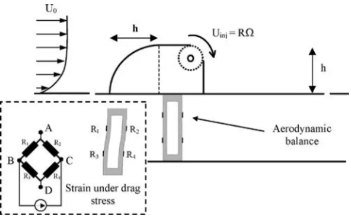
As we are interested in controlling separated flows, we choose to study the flow over a two-dimensional共2D兲 bluff body. The geometry is simple and consists in a quarter of a cylinder laying on the floor just in front of a square cylinder 共Fig. 1兲. The height of the bluff body is h=20 mm and its span length 100 mm. We use a small open wind tunnel whose cross section is 100 mm⫻100 mm. The upstream flow velocity U0ranges from 2 to 15 m s−1so that the
Rey-nolds number based on the bluff-body height Re = U0h / is
between 3000 and 20000.
This simple geometry creates a flow similar to the one behind a backward-facing step: the separation occurs at the edge and the flow reattaches further downstream. The sepa-ration surface is a region of strong unstable shears that are responsible for an important pressure drag.
We place a rotating cylinder at the edge of the backward-facing step in order to modify the separation properties共Fig. 1兲. The present study only concerns positive rotation, i.e., when the cylinder forces the flow in the same direction as the main flow. The radius of the cylinder is R = 5 mm and the rotation rate⍀/2can reach 250 Hz corresponding to a tan-gential velocity, or injection velocity, Uinj= R⍀ up to
7.5 m s−1. To obtain significant drag reduction, the ratio
Uinj/ U0should be of the order 1. The rotation of the cylinder
is provided by a computer-driven dc motor, using LabView. We evaluate the effect of the control on the drag using an aerodynamic balance composed of a plate mounted over a bimetallic brass strip共Fig. 1兲. Each strip is 0.3 mm thick and its behavior is similar to cantilever beams. The bluff body is maintained on the plate which is allowed to perform
horizon-FIG. 1. Sketch of the experimental setup. A rotating cylinder located at the edge of the step modifies the characteristics of the flow separation. The system is placed on a plateau fixed to bimetallic brass strips on which four strain gauges are glued. The global strain is measured with a full Wheat-stone bridge from Vishay共P 3100兲. The force 共i.e., the drag兲 depends lin-early on the strain. The full bridge configuration allows us to compensate temperature variations and to amplify the signal per a factor 2 compared to the half-bridge configuration. The output signal of the bridge is also ampli-fied by a factor 10 giving a sensitivity of 0.0527N / V, say 5.37g / V.
tal translations under a few tenths of a millimeter. When the flow is produced, the aerodynamic drag causes a translation of the plate, inducing a flexion of the sheets. Their deforma-tion is measured by four strain gauges glued on the strip, providing a signal whose average value is proportional to the mean drag 共see the inset in Fig. 1兲. The proper oscillation frequency of the brass structure is evaluated at 10.2 Hz 共when loaded with the model兲 from analyzing its response to an impulse.
In order to understand the modification of the flow due to the control device, we perform laser-induced visualization in the symmetry plane of the bluff body. We inject cold smoke共a spray of 0.3m di-ethyl-hexyl-sebacate droplets兲 into the bluff body itself共which is like an empty box兲 so that the smoke is naturally delivered into the flow through the thin gap共under 0.1 mm兲 between the model and the cylinder 共Fig. 2兲. This injection technique exhibits the recirculation zone very satisfactorily as displayed in Fig. 4共a兲. The images are captured with a CCD camera during a sufficiently long time共typically 1/30 s, whereas typical shedding periods are about few milliseconds兲 so that we obtain a picture of the time-averaged flow.
We finally use hot-wire anemometry to obtain mean ve-locity profiles downstream from the step. Each acquisition lasts until statistical convergence of the mean quantities 共typically a few tens of seconds兲.
III. OPEN-LOOP CONTROL: INFLUENCE OF THE ACTUATOR ON THE BASE FLOW
In this section, we study the effect of a uniform rotation of the cylinder on the drag and the mean flow structure and discuss the dependence of the results on two parameters, namely the mean flow velocity U0 and the rotation rate⍀.
A. Drag reduction
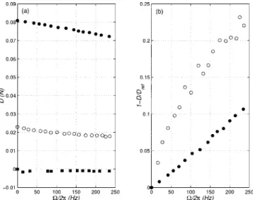
In Fig. 3共a兲, we show the evolution of the mean drag force D as a function of the rotation rate of the cylinder⍀ for three different free-stream velocities U0. First we can
notice that the rotation of the cylinder does not interact with the drag measurement. This is illustrated by the first curve 共black squares兲, which corresponds to the case with no flow
共U0= 0兲. We can see that the error is less than 10−3N, which
is negligible when the free-stream velocity is high enough. The other two curves show that for two different values of the free-stream velocity共U0= 6 and 12 m s−1兲, the drag is
a decreasing function of the rotation rate of the cylinder⍀. The drag reduction rate, defined as 1 − D / Dref 共with Dref the
drag without control兲, is then an increasing function of ⍀ 关Fig. 3共b兲兴. It reaches 23% and 11% for U0= 6 and 12 m s−1,
respectively. One can notice that the relative drag gain is nearly proportional to the rotation rate when U0= 12 m s−1
关Fig. 3共b兲兴.
B. Mean-flow modification
Smoke visualizations of Fig. 4 are realized for
U0= 2 m s−1 and show clearly the difference between the
natural separation关Fig. 4共a兲兴 and the “controlled” separation 关Fig. 4共b兲兴. The rotation of the cylinder clearly delays the
FIG. 2. Injection of cold smoke.
FIG. 3. Influence of⍀ on the drag for various free-stream velocities U0.共a兲
Drag measurements: black dots, U0= 12 m s−1; white dots, U0= 6 m s−1;
black squares, no flow共U0= 0 m s−1兲. 共b兲 Drag reduction rate: black dots,
U0= 12 m s−1; white dots, U0= 6 m s−1.
FIG. 4. Visualization of the separated flow downstream from the bluff body for U0= 2 m s−1.共a兲 Without control; 共b兲 with control 共Uinj/ U0= 2兲.
separation leading to a smaller recirculation bubble on the base of the bluff body and of course a smaller recirculation length.
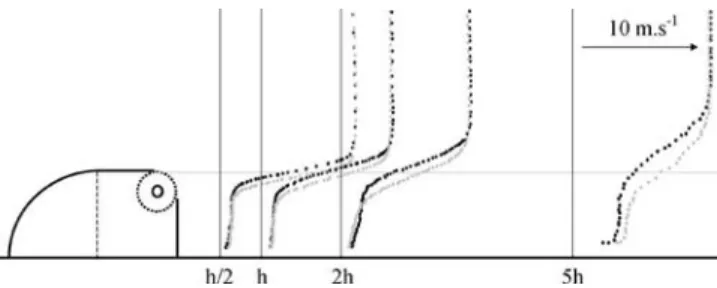
In Fig. 5 we show the modification of the velocity pro-files for higher free-stream velocity 共U0= 12 m s−1兲, for
which visualizations were not technically possible because of the turbulent diffusion of the smoke. The profiles exhibit the strong shear layer, which is clearly shifted downward when the cylinder is rotating共the black points, without control, are always above the gray points, with control兲. This is consis-tent with the fact that the separation point is also shifted downward. Hence, the results we obtain with hot wire an-emometry at high velocities seem to confirm the observation we made with flow visualizations for lower velocities. As the ratio Uinj/ U0is much smaller for high free-stream velocities, the modification of the base flow is less spectacular than the one observed in the flow visualizations performed with
U0= 2 m s−1.
The drag reduction mechanism seems to be simple: the rotation of the cylinder moves the detachment point further downstream and provides a recovery of the pressure drop on the base of the bluff body, inducing a drag reduction. This is consistent with the experimental results of Munshi et al.4 showing the separation delay, pressure rise, and drag de-crease obtained by momentum injection using sliding walls on the edges of rectangular prisms. As a matter of fact, the idea of using moving surfaces for boundary-layer separation control is not new: previous works4,13,22–24 are based on the hypothesis that a wall moving in the downstream direction causes a diminution of the relative motion between the wall and the free stream so that the boundary layer can undergo a more important adverse pressure gradient before breakdown. It is then an efficient tool for drag reduction or vortex-induced vibrations inhibition.4,13Hence the originality of our study does not lie on the choice of this device, but on the fact that we directly evaluate its effect on the drag, and above all that we use it as a well-known actuator for closed-loop con-trol experiments.
IV. PROPORTIONAL-INTEGRAL FEEDBACK CONTROL
A. Feedback scheme
The objective of the closed-loop control is to make a dynamical system able to reach and keep a predetermined state in spite of external perturbations. One of the major
difficulties is that measurements, information transfer, and activation of the actuator have to be simultaneously per-formed. In this section, we present a set of experiments that is a first step toward overcoming these difficulties.
We propose a closed-loop control allowing for the choice of a predetermined drag value for the system. Our experiment is characterized by a simple property of the drag evolution: it is a decreasing function of the cylinder rotation,
dD d⍀⬍0.
We propose the following feedback law to control the rotation as a function of the drag measurement:
d⍀
dt = K关D共t兲 − Dc兴, 共1兲
where D共t兲 is the measured drag, Dc the chosen drag target
value共i.e., a constant value the system must reach兲, and K a positive gain adjusted by the experimentalist. As underlined by Eq.共2兲, the cylinder rotation is determined at each time step from the distance between the measured drag and its target value Dc,
⍀共t兲 = K
冕
关D共兲 − Dc兴d. 共2兲This feedback scheme is called proportional-integral be-cause it consists in measuring the difference between the objective and the current state of the system, amplifying it before integrating it. The corresponding block-scheme is shown in Fig. 6.
It is possible to briefly justify the fact that such a closed-loop system should converge writing dDdt=dDd⍀ddt⍀. Since Dcis
constant in time, we can use the feedback law given by Eq. 共1兲 to finally obtain
d共D − Dc兲
dt = K dD
d⍀共D − Dc兲. 共3兲
We then show that 共D−Dc兲 is governed by a first-order
differential equation whose coefficient KdDd⍀ is negative, so that its solution should tend to 0. Hence the measured drag D should reach its target value Dc.
B. Experimental procedure
In a typical experiment, we begin with choosing a target value Dc, which is the drag value the system must reach. In
the definition of the loop 关Eq. 共1兲兴, one can see that if the drag is higher than the target, the rotation speed will increase and then the drag will decrease; when the system reaches its objective, the acceleration of the motor vanishes and the sys-tem becomes stable.
FIG. 5. Modulus of the mean velocity measured with hot wire anemometry for U0= 12 m s−1. Black dots: without control. Gray dots: with control
共Uinj/ U0= 0.5兲.
FIG. 6. Block-scheme of the closed-loop control. The drag measurement is used to give instruction to the motor.
From a practical point of view, the control algorithm is insured by a PC under LabView software with a National Instrument board. This PC acquires both the drag and the rotation speed of the motor at the rate of 500 Hz in a single point acquisition mode. Each measured point corresponding to a time step n, ⍀n, and Dn are used for the numerical
algorithm given by Eq.共4兲,
⍀n+1=⍀n+ K共Dn− Dc兲⌬t, 共4兲
where⌬t=tn+1− tn= 2⫻10−3s. The computed value of ⍀n+1
is generated at one analog output channel of the board at the updated rate of 500 Hz. This output is then used as the volt-age consign for the dc motor. These steps are summarized in Fig. 7. Finally, we use a second PC only devoted to the acquisition of both signals,⍀共t兲 and D共t兲 in a buffer acqui-sition mode at a sample frequency of 1 kHz.
C. Results and discussion
The data discussed in this section are obtained by start-ing the recordstart-ing without control, before startstart-ing the control a few seconds later. Without loss of generality, we only con-sider the case U0= 12 m s−1 and report results for various
values of the gain K. We show in Figs. 8–10 time series of drag normalized by its reference value D / Dref, and rotation
fluctuations.
At the beginning of each time series, there is no rotation and D is normally equal to its reference value Dref. As soon
as the closed-loop control is released, the system becomes autonomous and we observe that ⍀ increases sharply and goes above the objective Dc before decreasing regularly,
reaching the objective and stabilizing around it. In all cases, the rotation speed converges to 150 Hz, which corresponds to the rotation we should impose in the open-loop case to reach a 7% drag reduction共Fig. 3兲. The stabilization time is clearly dependent on the gain parameter K. By comparing the first two experiments, we can notice that as K increases from 0.5 to 5, the system becomes stable more quickly 共sta-bilization time decreases from 39 to 8 s兲. This observation is consistent with the previous discussion concerning the sys-tem convergence, as we can see in Eq.共3兲 that the higher K is, the faster is the convergence. We also have to notice that
FIG. 7. Sketch of the experimental procedure used for the PID closed-loop control.
FIG. 8. Time series for K = 0.5共arbitrary units兲. Upper figure: D/Dref, full
line; Dc, dashed line. Lower figure: rotation frequency⍀.
FIG. 9. Time series for K = 5共arbitrary units兲. Upper figure: D/Dref, full
line; Dc, dashed line. Lower figure: rotation frequency⍀.
FIG. 10. Time series for K = 100共arbitrary units兲. Upper figure: D/Dref, full
for higher K values 共Fig. 10兲 the system still reaches its objective but experiences very strong rotation fluctuations, due to a lack of stability.
This set of experiments shows that it is possible to create an experimental system able to reach autonomously a pre-defined stable state. It is also interesting to notice that it is in good agreement with the numerical experiment of Patnaik and Wei13studying the control of a square cylinder wake by momentum injection at the edges共in a laminar case兲. Their closed-loop scheme is similar to the proportionintegral al-gorithm and is based on the measurements of the velocity fluctuations in the whole domain, which is an integral quan-tity, as the drag force. In Ref. 13, the behavior of the rotation and that of the state of the system are similar to the behavior we report in this article, which underlines the encouraging results we obtained in the case of turbulent flows.
Nevertheless, one of the main limitations of the method is that by construction, the objective is imposed by the ex-perimentalist and must be chosen a priori. It is then impor-tant to search for new algorithms, more complex and more robust, allowing the system to identify and reach its final state without any previous instructions. This is the purpose of the following section.
V. REAL-TIME MINIMIZATION OF THE GLOBAL POWER OF THE SYSTEM
A. Power balance
By definition, active control requires an external energy input to activate the control device. It is then essential for the control to be useful that the actuation does not use more energy than the system gains thanks to the control: the power balance共difference between gain and loss of energy兲 must be positive. In our case, we want the highest drag reduction to reduce the dissipation through aerodynamic power
Pa= DU0. To reach this goal, we have to use electric power
Pe for the rotation of the actuator. The aerodynamic power
Padepends on both the rotation speed⍀ and the free-stream
velocity U0共see Fig. 3兲, while the electric power Peis found
to only depend on⍀ 共aerodynamic friction being negligible before solid friction兲. The measured electric power Pe= VI,
where V and I are, respectively, the voltage and the current applied to the dc motor, can be fitted by a quadratic law,
Pe=␣⍀2 共Fig. 11兲. In the following, the electric power is
always estimated from the angular velocity of the dc motor using this fitted law. We can then define the power balance function J共⍀,U0兲 as the sum of electric and aerodynamic
power,
J共⍀,U0兲 = Pa共⍀,U0兲 + Pe共⍀兲 = D共⍀,U0兲U0+␣⍀2. 共5兲
From the experimental point of view, the instantaneous J function as defined in 共5兲 is computed on a PC using a single-point acquisition mode of the rotation frequency ⍀, the free-stream velocity U0, and the drag measurements D
with a 200 Hz update rate.
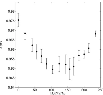
As the aerodynamic power is a decreasing function of the rotation frequency⍀ 共Fig. 3兲 and the electric power an increasing function of⍀ 共Fig. 11兲, the J共⍀兲 function must have a minimum for all free-stream velocities. We measured
the averaged value of the J function as a function of⍀ for a given free-stream velocity U0= 12 m / s. We obtain the curve shown in Fig. 12, which clearly has a minimum, even if poorly defined, between 100 and 150 Hz. For this magni-tude of rotational frequencies, the drag reduction is about 5%, as can be seen in Fig. 3共b兲. The objective of the closed-loop experiment is then for the system to reach autono-mously this minimum. We should then be able to use an “extremum-seeking control” strategy to help the system to find its minimum.
B. Extremum-seeking control scheme and experimental procedure
In the previous section, we defined our new objective: to minimize the total power dissipated by the system for any free-stream velocity U0. The control parameter ⍀ must be
FIG. 11. Electric power used by the motor as a function of the rotation frequency: measurements共black points兲 and quadratic fit 共continuous line兲
Pe=␣⍀2, where␣= 4.44⫻10−8W /共rad s−1兲2.
FIG. 12. Evolution of J as a function of the rotation speed ⍀ for
adjusted by the system to reach the state of minimum power injected corresponding to the minimum of the J function. In this respect, we choose to use an “extremum-seeking con-trol” strategy that is efficient in the case in which a nonlinear plant has an extremum. It consists in using a real-time gra-dient optimization method with the following feedback law:
d⍀ dt = − K
J
⍀, 共6兲
where K is a positive gain that is chosen by the experimen-talist.
In the case of turbulent flows, the fluctuations of physi-cal quantities are large with a broad spectrum. This situation makes the evaluation of the gradient by classic finite differ-ence nearly impossible. Krstić and Wang21have recently re-visited the sinusoidal perturbations method, which allows us to deal with largely fluctuating signals. It consists in modu-lating the input of our system in the following way:
⍀共t兲 = ⍀0共t兲 + a cos共2fmt兲. 共7兲
From now on, ⍀ is no longer constant, but is modulated around⍀0共t兲. The modulation amplitude a and frequency fm
are chosen by the experimentalist and are constant during the experiments. The constant a has to be sufficiently large and
fmlower than the cutoff frequency of the balance to detect
the effect of the modulation on the drag measurements. We then took a / 2= 40 Hz and fm= 1 Hz. The objective is that
⍀0共t兲, which is a slowly variable function of time, reaches
the value corresponding to the minimum of the J function, regardless of the free-stream velocity U0. We will speak
about modulated open loop when the rotation is modulated and⍀0 constant in time.
To estimate the gradient of ⍀J共⍀0兲, a second PC
ac-quires J共t兲 共from the first PC兲 and ⍀共t兲 in a single-point acquisition mode at a sampling rate of 50 Hz. This PC per-forms fast Fourier transform of both quantities over a sliding window of 4096 points corresponding to a 81.92 s time win-dow. A temporal window of J and its amplitude spectrum is displayed in Fig. 13 during modulated open loop. The spec-trum of J is dominated by the drag measurements. The nar-row peak at 10 Hz, corresponding to the lowest-frequency mode of the balance, is followed by a wide peak. We do not have any clear idea about the origin of this wide peak that could correspond other modes of the balance. However, the presence of these peaks is not a limitation since we are in-terested in the measurements at lower frequencies that are the mean and the amplitude at the modulation frequency. The modulation peak at fm= 1 Hz is clearly distinguishable
共modulated peak in Fig. 13兲. Both the amplitude AJ共fm兲 and
the phaseJ共fm兲 of the mode fmare then extracted from the
spectrum of the sliding windows. The values are updated at a rate of 50 Hz. Simultaneously, the same treatment is per-formed on ⍀共t兲 in order to extract its phase ⍀共fm兲 at the
modulation frequency. The relationship between these mea-sured quantities and the gradient is the following. The devel-opment of the J function around the actual value⍀0reads
J共⍀兲 = J共⍀0兲 + 共⍀ − ⍀0兲
J
⍀共⍀0兲. 共8兲
Since ⍀ is modulated as in Eq. 共7兲, the response of the J function to the modulation is for a small enough,
J关⍀0+ a cos共2fmt兲兴 = J共⍀0兲 + a cos共2fmt +兲
⫻
冐
J⍀共⍀0兲
冐
, 共9兲with= 0 or. In this case J is also a harmonic function of time whose amplitude of the mode fm is proportional to
储⍀J共⍀0兲储. Also, the phase shift =⍀共fm兲−J共fm兲, being
the phase difference between both modes of⍀ and J at the frequency fm, gives the sign of the gradient, and we have
J
⍀⬇
AJ共fm兲
a sgn兵cos关⍀共fm兲 −J共fm兲兴其. 共10兲
Finally the second PC gives 50 orders per second to the motor controlling the rotation of the cylinder according to the following relation:
⍀n+1=⍀0,n+1+ a cos关2fm共n + 1兲⌬t兴, 共11兲
⍀0,n+1=⍀0,n− K
AJ共fm兲
a sgn兵cos关⍀共fm兲 −J共fm兲兴其⌬t,
共12兲 where⌬t=tn+1− tn= 2⫻10−2s. More details about this
tech-nique are given in Refs. 20 and 21. The different steps of this closed-loop control algorithm are summarized for its prin-ciple in the block diagram in Fig. 14 and for its experimental procedure in Fig. 15.
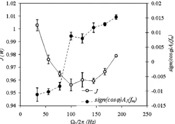
In order to characterize the robustness of the gradient estimator, we recorded J and sgn共cos兲AJ共fm兲 during 100 s
in an open-loop control experiment 共see Fig. 13兲. We re-peated this recording for different rotation frequencies⍀0of
the actuator. We display the average of J together with
FIG. 13. Upper figure: typical time series of the J function. Lower figure: J spectrum of the time series computed on a 4096-point sliding window. The modulation peak corresponding to the modulation frequency fm= 1 Hz is
sgn共cos兲AJ共fm兲 in Fig. 16. The measurements are
accom-panied with error bars that correspond to their root-mean square values. We can check that the algorithm is able to detect the minimum of J. However, the gradient magnitude is not well estimated around this minimum where it should go to 0.
C. Results and discussion
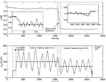
In a first experiment, we use the experimental procedure described in Fig. 15 and the relation共12兲, with U0= 12 m / s 共Fig. 17兲. At the beginning of the experiment, there is no forcing 共⍀=0兲 and J=Jref⯝0.98 W. After some times, we apply the modulated open-loop control with⍀0= 45 Hz and observe the decreasing共in less than 80 s兲 of the J function toward a value close to 0.96 W, which corresponds to the mean value we measured in open-loop control for ⍀0= 45 Hz共Fig. 12兲. Then we trigger the closed-loop control
and observe a new decrease of J, which finally begins to oscillate around a mean value close to 0.95 W. During this last step, the system is completely autonomous and no longer needs any external intervention. The mean value of the rota-tion⍀0increases as soon as the loop is closed and oscillates
around 100 Hz. One can underline that the mean value J corresponding to⍀0= 100 Hz in the open-loop experiment is
about 0.95 W, corresponding to the second plateau of the J function共Fig. 12兲. The large fluctuations of ⍀0 can be
ex-plained by the fact that the minimum of the J function is not well defined.
We now perform the same experiment with a slight dif-ference: after some times, we modify the free-stream
veloc-ity to check if the system is able to fit to these changing flow conditions and can identify and reach its new optimal state without any external intervention.
The experiment begins with no forcing共Fig. 18兲 leading to J = Jref⯝0.98 W. After a short time of modulated
open-loop control 共with ⍀0= 45 Hz兲, we start the
extremum-seeking control loop. Just like in the previous experiment,
J reaches the value 0.95 W while ⍀0increases before
fluc-tuating around the mean value⍀0= 100 Hz. After a 1600 s
recording, the free-stream velocity is lowered from
U0= 12 m / s to U0= 10 m / s 共Fig. 18兲 so that the drag
de-creases sharply and, consequently, J = DU0+Pestrongly
de-creases. The loop is still closed and the system reaches au-tonomously a new mean rotation speed ⍀0= 70 Hz around
which it fluctuates. The value of the J plateau is about 0.50 W. Finally ⍀ is set to 0 to turn the forcing off. J in-creases and reaches again its reference value about 0.51 W for U0= 10 m / s. The corresponding value of the J plateau is
about 0.51 W. This new plateau is higher than the value
FIG. 15. Description of the experimental procedure used for closed-loop control using the sinusoidal perturbations method.
FIG. 16. Open-loop control results about estimation of the gradient of J versus J at the mean rotation frequency⍀0of the actuator.
FIG. 17. Open-loop and closed-loop control experiment for U0= 12 m / s. Upper figure: J, fine continuous line; plateau of J, dashed line. Lower figure: rotation⍀0, continuous line; plateau of⍀0, dashed line.
FIG. 14. Sketch of the feedback closed-loop control using the sinusoidal perturbations method.
reached by the system in closed loop, which is the evidence of the efficiency of the loop, even if we cannot assert that it is exactly the optimal state.
The experimental results reported in this section show that the extremum-seeking closed-loop control strategy based on the sinusoidal perturbations method is efficient, us-ing our experimental procedure. In both experiments it makes the system able to evaluate its global power budget in real time共through the measurements of the J function兲 and then to identify and reach its optimal set point, which corre-sponds to the maximum power saving, without any external intervention. Finally, it appears that this adaptive control method allows the system to fit to variable flow conditions, such as the mean-flow velocity.
VI. CONCLUDING REMARKS
In this article, we report experimental results concerning open- and closed-loop control of a bi-dimensional turbulent separation, in order to reduce the drag of a bluff body. We first demonstrate the efficiency of moving walls to delay separation and then reduce the drag. The effect of a rotating cylinder placed on the edge of the bluff body is larger as the rotation is increased, which allows remarkable actuation for closed-loop experiments.
Next we try a proportional-integral algorithm to impose a predefined state on the system. In this case, the experimen-talist chooses a target value the system should reach and the drag measurement is used to build the instructions given to the motor. Using our experimental procedure, the system is actually able to reach its objective.
Then we propose an energy condition so that the system will search for the optimal state corresponding to the com-promise between the maximum drag reduction and the mini-mum electric power consumption. In this second set of ex-periments, we propose a real-time gradient method that can
be applied thanks to a sinusoidal perturbations method. It consists in modulating the input of the system before per-forming a spectral analysis of the output in order to evaluate the gradient of the function we want to optimize. Using the estimated gradient, we modify the input in real time so that the system reaches and oscillates around its optimal state. We demonstrate the efficiency of the algorithm by performing an experiment with time-dependent external conditions: the free-stream velocity is modified and the system reaches au-tonomously its new optimal state.
Both of the adaptive methods that are detailed in this study seem to be efficient since they make the system able to react in real time. As the proportional-integral algorithm re-quires little data processing, it is a rather fast method. But its main limitation lies in the fact that the set point the system reaches has to be defined a priori. On the contrary, the extremum-seeking scheme allows the system to identify its objective by its own in the general case in which a nonlinear plant presents an optimum. Since in this case the data pro-cessing is rather important共in particular because of the spec-tral analysis兲, this closed loop is much slower than the first one, but appears to be efficient.
From an academic point of view, we emphasize the fact that not many experiments in fluid mechanics attest to the real efficiency of active control in globally reducing the en-ergy consumption of a system. In this sense, our experiment is a very convincing illustration.
As a result, we believe that both of these methods are interesting for other applications and we demonstrate that they overcome the main difficulties associated with the closed-loop control of turbulent flows. Hence we are confi-dent that such adaptive schemes could be a powerful tool for some industrial applications. In particular, Beaudoin25 has recently used the same extremum-seeking control experi-mental procedure to reduce the drag of a simplified vehicle 共with a totally different type of actuator兲 with success.
ACKNOWLEDGMENTS
We would like to thank P. Rouchon and B. Protas for fruitful discussions. We also acknowledge the useful help of D. Pradal and D. Vallet in preparing the model for the experiments.
1T. R. Bewley, “Flow control: New challenges for a new Renaissance,”
Prog. Aerosp. Sci. 37, 21共2001兲.
2M. Gad-El-Hak, “Flow control,” Appl. Mech. Rev. 42, 261共1989兲. 3M. Gad-El-Hak and D. M. Bushnell, “Separation control: Review,” J.
Fluids Eng. 113, 5共1991兲.
4S. R. Munshi, V. J. Modi, and T. Yokomizo, “Aerodynamics and dynamics
of rectangular prisms with momentum injection,” J. Fluids Struct. 11, 873 共1997兲.
5B. Protas and J. E. Wesfreid, “Drag force in the open-loop control of the
cylinder wake in the laminar regime,” Phys. Fluids 14, 810共2002兲.
6D. Greenblatt and I. J. Wygnanski, “The control of flow separation by
periodic excitation,” Prog. Aerosp. Sci. 36, 487共2000兲.
7T. R. Bewley, P. Moin, and R. Temam, “DNS-based predictive control of
turbulence: An optimal benchmark for feedback algorithms,” J. Fluid Mech. 447, 179共2001兲.
FIG. 18. Open-loop and closed-loop control experiment with a change of the free-stream velocity during the experiment 共from U0= 12 m / s to
U0= 10 m / s兲. Upper figure: J, continuous line; J plateau, dashed line 共the
two windows in the main window are an enlargement of the beginning and the end of the signal兲. Lower figure: rotation ⍀0, continuous line;⍀0
8H. Choi, P. Moin, and J. Kim, “Active turbulence control for drag
reduc-tion on wall-bounded flows,” J. Fluid Mech. 262, 75共1994兲.
9N. Fujisawa, Y. Kawaji, and K. Ikemoto, “Feedback control of vortex
shedding from a circular cylinder by rotational oscillations,” J. Fluids Struct. 15, 23共2001兲.
10N. Fujisawa and T. Nakabayashi, “Neural network control of vortex
shed-ding from a circular cylinder using rotational feedback oscillations,” J. Fluids Struct. 16, 113共2002兲.
11M. Garwon, L. H. Darmadi, F. Urzynicok, G. Bärwolff, and R. King,
“Adaptive control of separated flows,” in Proceedings of the 2003 Euro-pean Control Conference, Cambridge, UK共2003兲.
12J. Kim, “Control of turbulent boundary layers,” Phys. Fluids 15, 1093
共2003兲.
13B. S. V. Patnaik and G. W. Wei, “Controlling wake turbulence,” Phys. Rev.
Lett. 88, 054502共2002兲.
14B. Protas and A. Styczek, “Optimal rotary control of the cylinder wake in
the laminar regime,” Phys. Fluids 14, 2073共2002兲.
15M. M. Zhang, L. Cheng, and Y. Zhou, “Closed-loop-controlled vortex
shedding and vibration of a flexibly supported square cylinder under dif-ferent schemes,” Phys. Fluids 16, 1439共2004兲.
16Y. Wang, G. Haller, A. Banaszuk, and G. Tadmor, “Closed-loop
Lagrang-ian separation control in a bluff body shear flow model,” Phys. Fluids 15, 2251共2003兲.
17C. M. Ho and Y. C. Tai, “Review: MEMS and its applications for flow
control,” J. Fluids Eng. 118, 437共1996兲.
18C. M. Ho and Y. C. Tai, “Micro-electro-mechanical-systems共MEMS兲 and
fluid flows,” Annu. Rev. Fluid Mech. 30, 579共1998兲.
19M. Krstić, I. Kanellakopoulos, and P. V. Kokotovic, Nonlinear and
Adap-tive Control Design共Wiley, New York, 1995兲.
20J. F. Beaudoin, O. Cadot, J. L. Aider, and J. E. Wesfreid, “Bluff-body drag
reduction by extremum seeking control,” J. Fluids Struct.共in press兲.
21M. Krstić and H. H. Wang, “Stability of extremum seeking feedback for
general nonlinear dynamic systems,” Automatica 36, 595共2000兲.
22A. Alvarez-Calderon, “Rotating cylinder flaps of V/STOL aircraft,” Aircr.
Eng. 36, 304共1964兲.
23B. Choi and H. Choi, “Drag reduction with a sliding wall in flow over a
circular cylinder,” AIAA J. 38, 715共1999兲.
24V. J. Modi, F. Mokhtarian, M. S. U. K. Fernando, and T. Yokomizo,
“Moving surface boundary-layer control as applied to two-dimensional airfoils,” J. Aircr. 28, 104共1991兲.
25J. F. Beaudoin, “Contrôle actif d’écoulement en aérodynamique