Two Bayesian methods for multipath propagation parameters estimation

(1)

HAL Id: hal-02141163

https://hal.archives-ouvertes.fr/hal-02141163

Submitted on 27 May 2019

HAL is a multi-disciplinary open access

archive for the deposit and dissemination of

sci-entific research documents, whether they are

pub-lished or not. The documents may come from

teaching and research institutions in France or

abroad, or from public or private research centers.

L’archive ouverte pluridisciplinaire HAL, est

destinée au dépôt et à la diffusion de documents

scientifiques de niveau recherche, publiés ou non,

émanant des établissements d’enseignement et de

recherche français ou étrangers, des laboratoires

publics ou privés.

Two Bayesian methods for multipath propagation

parameters estimation

Fabienne Porée, Olivier Rosec, Thierry Chonavel, Jean-Marc Boucher

To cite this version:

Fabienne Porée, Olivier Rosec, Thierry Chonavel, Jean-Marc Boucher.

Two Bayesian

meth-ods for multipath propagation parameters estimation.

ICASSP 2000 : IEEE International

Con-ference on Acoustics, Speech and Signal Processing, Jun 2000, Istanbul, Turkey.

pp.69 - 72,

�10.1109/ICASSP.2000.861866�. �hal-02141163�

(2)

TWO BAYESIAN METHODS FOR MULTIPATH PROPAGATION

PARAMETERS ESTIMATION

F. Pore'e,

0. Rosec,

T .

Chonavel and

J.M.

Boucher

ENST de Bretagne

Technopde de Brest Iroise, BP 832

29285 Brest cedex, France

ABSTRACT

In this paper we propose a bayesian approach for multipath channel time delay estimation when the signal is received by a square-law detector. Two different methods are presented. The first one is applied when t.he signal is supplied at the output of the detector. On cert,ain approximations, the derivation of the MAP (Maximum A Posteri- ori) estimator leads to optimize a l1-norm criterion. In the second method, the signal is observed after demodulation and matched-filtering. We introduce a Bernoulli-Gaussian model to account for the sparse properties of the channel impulse response and solve the deconvolution problem using Monte-Carlo simulations. Comparisons between both algorithms are presented on simulations. They show that the second method leads to more accurate estimators, while justifying the validity of the approximations used in t,he first one.

1. INTRODUCTION

Many problems can be modeled as a linear system where

the observed output signal r ( t ) is the convolution of the input signal e ( t ) with a sparse spike time series h ( t ) . De- pending on the.domain of application, the function h( t ) can be for instance the reflectivity sequence of a seismic trace

[ 8 ] , or a propagative channel multipath impulse response as in oceanic acoustic tomography [15]. In such cases, h ( t ) can be written as

P

h ( t ) = 1 a p S ( t - .PI, ( 1 ) p= 1

where a p and rP are respectively the attenuation and the delay associated to the p t h path, and P is the number of paths. In applications such as ocean acoustic tomography

[15], e ( t ) is known by the receiver. Then the problem of estimating the ( a p , ~ ~ ), p , ~ and possibly the number = l P of paths, can be addressed via maximum likelihood estimation (see e.g.

[a]

[9]). Unfortunately, the log-likelihood criterion

shows local maxima, and it requires the knowledge of the number of paths.

To overcome these limitations, we propose a bayesian approach [13] which allows to include information upon the parameters by means of a priori distributions. Here we take into account the fact that the paths amplitudes ( a p ) p = l , p

and the noise have gaussian distributions. In this work, we present two different deconvolution methods. The first one addresses the case where the only available signal is obtained a t the output of a square-law detector. On cer- tain approximations, the derivation of the MAP estimator leads to a very simple l1-norm criterion. In the second method the signal is complex-valued, and is obtained after demodulation and matched-filtering. We introduce a Bernoulli-Gaussian model to account for the sparse p r o p erties of h ( t ) and solve the deconvolution problem using Monte-Carlo simulations.

The reason for considering both approaches stems from the fact that the first method involves linear approximations of the non-linear transforms in the square-law detector. The simulation results demonstrate the superiority of the Bernoulli-Gaussian model. However we show that processing the signal a t the output of the quadratic receiver is quite robust to the above approximations, and thus can be used when only the output of the square-law detector is available.

The problem is presented in section 2 . In section 3 et 4 , the two different bayesian methods are developped. Results

and comparison are discussed in section 4.

2. FORMULATION OF THE PROBLEM

Let s ( t ) denote the transmitted signal, r ( t ) the received signal, and v ( t ) an additive gaussian white noise with variance cz, independent from h ( t ) . At the transmitter side s ( t ) is modulated by a carrier with pulsation w . Then, the received signal r ( t ) is in the form:

At the receiver side, r ( t ) goes through the square-law de- tector according to the scheme of the figure l , where 9 ( t ) = s ( - t ) is the impulse response of the matched-filter.

Let g ( t ) denote the complex signal obtained a t the out- puts of the matched-filters. It can also be written in the form:

(3)

2cosot

-2 sin'ot

Figure 1: Structure of the receiver.

p = 1

g p = o p cos(w.rP

+

4 )

+

i a p sin(wTp

+

4).

Finally, t,he sampled observation in the observation in-

P

d n ) = EPd. - .PI

+

b ( n ) , (4)

terval, say [I, NI,

x

= ( ~ ( n ) ) , = ~ , ~ , can be written

p = 1

where

b(

n ) is a complex circular gaussian random variable, with variance g i

_-

= 40; (g is normalized with g ( 0 ) = 1).

3. L1 N O R M D E C O N V O L U T I O N AT THE

O U T P U T OF THE R E C E I V E R

3.1. T h e received s i g n a l y ( t )

In this first approach we consider, as already in 1111, the case where t.he only available signal is obtained a t the output of t,he quadratic receiver, and denoted y ( t ) . With a view to getting a simple expression of this signal, we consider two approximations. First, the product terms between the signal of interest and the noise are neglected, which is generally justified because of t,he high SNR a t the output of the mat.ched filter. Moreover, the product terms associated wit.h two distinct paths are neglected, which is generally a sat.isfactory approximation when the autocorrelation function of s ( t ) is sharp. Then, y(t) can be written as:

d t ) = ( h

*

.)(t)

+

4 t )

P

= a p z ( t - TP)

+

c ( t ) , (5)

p = 1

with ~ ( t ) = g 2 ( t ) and a p = Iap12.

3.2. T h e I1-norm c r i t e r i o n

-4ssuming t.hat the noise b ( t ) and the attenuations c y p [12]

have gaussian dist,ributions:

a p

-

J W l U 3 , (6)

b ( t )

-

N O , g : ) , ( 7 ) a p

-

& ( 1 / 2 d ) , ( 8 )

€ ( t )

-

& ( 1 / 2 4 ) . (9)

it comes that aP and e ( t ) have exponential distributions:

Without prior information upon the time delays, we assume that they are uniformly distributed in the observation interval: rp

-

U [ ~ , N I .

Then, the posterior likelihood minimization problem is:

In order to optimize the criterion, the time scale is dis- cretized in the same way as in [3] [6]. Finally, we get the problem in the form

In this criterion, X = U : / & , S, is the matrix of convolu-

tion with the sampled

g ( t ) ,

y is the d a t a vector, and h is the vector of the amplitudes of the paths on the sampled time scale. Moreover let us remark that the spike train can be solved with higher resolution than the received d a t a sampling intervalle [3] [14].

Also, let us note that the criterion (11) as already been considered in the litterature. In [14], the l1-norm term

11

y

-

S,h is justified by the spike preservation properties, and the penalty term X

11

h

Ill

by the fact that h ( t ) is

sparse. Moreover, X appears as the weighting factor selected to balance the conflicting priorities of data accountability and addresssing the a priori assumption that h ( t ) IS . sparse

[IO]. But in such methods the choice of the value of the parameter X is often a problem. Here, the bayesian formu- lation of the problem leads to a simple interpretation of A, as the inverse of a signal to noise ratio. Thus, it is generally possible to estimate X in a simple way.

This criterion can be also rewritten in the form:

with

A = ( : ; ) , a n d c = (

K )

The minimization of the criterion (12) is implemented according to the algorithm presented in [I], that uses the simplex method applied to a linear programming formulation of the problem. Also, with a view to adaptative track- ing of time-varying channels parameters, the convex criterion

I/

c - Ah

Ill

can be minimized by means of a simple gradient algorithm.

4. B E R N O U L L I - G A U S S I A N

D E C O N V O L U T I O N

4.1. M o d e l p r e s e n t a t i o n

Instead of deconvolving the signal after quadratic detec-

tion, we consider here the complex signal at the output

of the matched filters. In this case, we are faced to a deconvolution problem in the presence of gaussian noise. T h e convolutional model ( 3 ) can be rewritten as:

(4)

When no prior is available upon

h

the deconvolution is equivalent to the maximization of the likelihood function given by:

where S, denotes the convolution matrix deduced from g . The maximum likelihood estimate is not an appropriate solution, although it can be shown that it is the minimum variance unbiased estimator.

A major drawback of maximum likelihood deconvolution is that it does not take into acount the fact that

h(n)

is a sparse sequence of arrival time. A possible way to reg- ularize the problem is to introduce a Bernoulli variable q to

indicate the presence of a path. Then

h(n)

can be modeled

by a Bernoulli-Gaussian process defined by:

where

q = P ( q ( n ) = 1) = 1 - P ( q ( n ) = 0) (17)

is the prior probability of finding a path a t each sample n.

Stricly speaking a pure Bernoulli-Gaussian is obtained when

a: = 0. However, as the likelihood of a Dirac distribution is not defined we introduce a non-zero variance a:

<<

a:. In geophysics this model is commonly used to characterize the reflectivity of the subsurface, and a; describes small hetero- geneity in the sedimentary layers 141. In nuclear science

ai

models some background disturbance noise a t the receiver.

4.2. The MCMC approach

I n that framework, the problem is to study the post.erior likelihood p ( h , qlx). Using Bayes rule and omitting the

constant t.erm p ( 3 ) this density can be writ.ten as:

P(h, qlx) P(Xlh)P(hlq)P(q). ( 18)

After some easy calculations the posterior log-likelihood becomes:

with D = diag(q). Let us not.ice that given a vector q,

L

is a quadrat.ic function of

h

and so its maximum can be ob-

tained in closed form. Unfortunately the st,udy of

C

for the

2 N possible q sequences is computationnally untractable as soon as N becomes large.

To overcome this difficulty it is possible t.0 use simulation methods. For the application we are interested in, sup- pose we are able to generat.e a sequence of independent samples

{(hem),

q")), m = 1 , . . .

,

M } according to

p((h,

q)lX).

Then we can use these samples to make inference on the missing variables such as calculating conditionnal expecta- tions q q l ~ ] and

qhI1EJ.

Therefore our problem comes down to the simulation

of

(h,q)

according to their posterior distribution. However

generating high dimension variables remains a difficult task as soon as the distributions are non-standard. Here the convolution introduces time dependency of the missing variables conditionally on the observation, and no direct simu-

lation scheme is possible. One way of solving this problem

is to use MCMC methods. The basic principle is to gener- ate a Markov Chain whose equilibrium distribution is the target distribution. The most popular MCMC algorithms as well as details concerning their convergence properties can be found in [13].

4.3. The Gibbs sampler

One simulation scheme is to simulate the missing variables one sample a t a time. Indeed it can be shown (see [5]) that conditionally on { h ( j ) , q ( j ) , j

#

n}, (h(n),q(n)) can

be written as a mixture of gaussian distributions. This motivates the choice of a Gibbs sampler. The algorithm proceeds as follows:

1. Initialization : random choice of

(h('),q('))

;

2. At iteration m

5

M , for n = 1 , . . .

,

N

:

e choose site i ;

simulate

(h(i),q(i))

according to

P(h(4,

s(9ln,

hb),

q ( j ) , j

#

2 ) .

At each iteration, the sites are visited using a random per- mutation of (1, .. . , N}. The behavior of the algorithm can be divided into two periods: first a burning period of

MO

iterations and then a steady state period where it can be assumed that the drawn sampled are distributed according to their posterior distribution.

Then, we calculate for each sample 1

5

n

5

N M

Then we use the following decision rule:

if Q(n)

>

0.5 set {(n) = 1 and &(n) = Q ( n ) H ( n ) e else set G(n) = 0 and

h(n)

= 0 .

5 . RESULTS

We now apply these two methods to numerical data. Let

s ( t ) be a M.L.S. (Maximium Length Sequence) [12] of length

n = 2' - 1 = 511 symbols with values kl/@. The auto-

correlation of the M.L.S. is a triangular shape, carried by the interval [-I<, K], where I< is the symbol duration. We assume that y ( t ) is sampled a t a rate 6 = K / 6 .

We simulate two arrival times 7 1 and 7 2 with amplitudes

1, for a SNR equal to 30 dB, ie a: = The results are

presented for 2 values of the difference

1

7 1 - 7 2

I.

Fig-

ure 2 shows an example of the signals obtained at different locations of the detector.

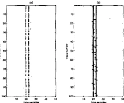
For each scenario, the performances are tested on 100 traces, corresponding to 100 independent realizations of the

(5)

6. CONCLUSION

11 MCMC

-

I

i-1 - i-2

I

I< K / 2 I i / 2

PO, 100 96 100 100

PO2 91 88.5 98.5 97.5 - 0 5 a ' 8 " " "

0 5 10 15 20 25 30 35 40 I5 50

3 , , , , , , , ~,

Figure 2: (a) Real part of ~ ( t ) ; (b) Imaginary part of g ( t ) ;

(c) Output real signal y ( t ) .

noise. Figure 3 represents the image of the results obtained with each method.

The 21-norm method is implemented using standard Nag fortran routines 171. The parameter X is chosen equal to

l/2aE. For the Bernoulli-Gaussian deconvolution algorithm, the model parameters are respectively U: - = 4.10-3, uf = 1,

ri

= and '7 = 0.04. We run the Gibbs sampler for

M = 500 iterations and discard the first 100.

Figure 3: Results obtained on the 100 traces with

I

TI - 7 2

I=

IC/2: (a) Z1-norm method ; (b) MCMC method.

In this paper we have presented two methods for time delay estimation. We have seen that a t the output of the square- law detector a very simple approximate MAP criterion can be considered, that yields good results in terms of path detection and delay estimation. Moreover when the complex data a t the output of the matched-filter are available, bet- ter accuracy can be achieved via MCMC simulations of the parameters posterior distribution.

7. REFERENCES

[l] I. Barrodale and F.D.K. Roberts. An improved al-

SIAM

gorithm for discrete 11 linear approximation.

Numer. Anal., 10(5):839-848, Oct. 1973.

superimposed signals using the em algorithm.

Trans. on A .S.S.P., 36(4):477-489, 1988.

[3] J-J. Fuchs. Multipath t.ime-delay detection and esti-

mation. ZEEE Trans. S.P., 47(1):237-243, Janv. 1999.

[4]

M.

Lavielle. Bayesian deconvolution of bernoulli-

gaussian processes. Signal Processing, 33:67-79, 1993.

[5] M. Lavielle. A stochastic algorithm for parametric and

non-parametric estimation in the case of incomplete data. Signal Processing, 42:3-17, 1995.

Multipath time delay estimation using regression stepwise procedure. IEEE Trans.

S.

P.,

46(1):191-195, January 1998.

[7] The Numerical Algorithms Group Limited. The Nag

Fortran Library Manual, Mark 1 4 , 1st edition, April

1990.

[8] J.M. Mendel. Maximum-likelihood deconvolution : a

journey into model-based signal processing. Springer-

Verlag, 1990.

Active estimation of a multipath propagation channel with a bayesian strat- egy. Traitement du signal, 10(3):201-213, 1993.

[IO] M. O'Brien, A. N. Sinclair, and S.

M.

Iiramer. Re- covery of a sparse spike time series by 11 norm decon-

volution. ZEEE Trans. S.P., 42( 12):3353-3365, Dec.

1994.

[ll] F. Poree, T. Chonavel, and T. Terre. Multipath time- delay detection and estimation for ocean acoustic to-

mography: a bayesian approach. In Oceans'99 MTS/

IEEE Proceedings, volume 3, pages 1587-1590, 1999.

[la] J . G. Proakis. Digital Communications. Mac Graw

Hill, second edition, 1989.

[13] C. P. Robert. The bayesian choice. Springer-Verlag,

New-York, 1994.

[14] H. Taylor, S. Banks, and F. McCoy. Deconvolution with the 11 norm. Geophys., 44(1):39-52, 1979. [15] C. Wunsch W. Munk, P. Worcester. Tomography

[2] M. Feder and E. Weinstein. Parameter estimation of

IEEE

[6] Tze Fen Li.

[9] V. Nimier and G. Jourdain.

Acoustic Oceanic. Cambridge University Press, 1995.

Table 1: Detection results.