Measurements and calibration method for WLAN indoor path loss modelling

HAL Id: hal-02379345

https://hal.archives-ouvertes.fr/hal-02379345

HAL is a multi-disciplinary open access archive for the deposit and dissemination of sci-entific research documents, whether they are pub-lished or not. The documents may come from teaching and research institutions in France or abroad, or from public or private research centers.

L’archive ouverte pluridisciplinaire HAL, est destinée au dépôt et à la diffusion de documents scientifiques de niveau recherche, publiés ou non, émanant des établissements d’enseignement et de recherche français ou étrangers, des laboratoires publics ou privés.

Measurements and calibration method for WLAN

indoor path loss modelling

Rida Tahri, Valery Guillet, Jean-Yves Thiriet, Patrice Pajusco

To cite this version:

Rida Tahri, Valery Guillet, Jean-Yves Thiriet, Patrice Pajusco. Measurements and calibration method for WLAN indoor path loss modelling. IEE Sixth international conference on 3G and beyond, Nov 2005, Washington, United States. pp.1 - 4. �hal-02379345�

MEASUREMENTS AND CALIBRATION METHOD FOR

WLAN INDOOR PATH LOSS MODELLING

R. Tahri, V. Guillet, J. Y. Thiriet and P. Pajusco

France Télécom 6, avenue des Usines - BP 382 - 90007 Belfort, France { rida. tahri, valery. guillet, j ean-yves. thiriet, patrice. pajusco }@francetelecom.co m

Keywords: Indoor measurements, WLAN.

Abstract

propagation, modelling,

For indoor Wireless LAN systems planning, an accurate propagation modelling is required. Semi-empirical models represent an efficient approach to the coverage prediction. Based on measurement results, the model parameters are derived. In this paper we present the influence of the measurements points choice on the accuracy of the parameters estimation and thus on the model robustness.

1 Introduction

Over the last few years, the market for wireless service has grown at an unprecedented rate. The commercial success achieved by the introduction of cellular mobile radio telephones has generated strong interest in the development of other wireless communications systems. Recently, there has been an increasing interest in providing wireless local area networks (WLAN) working in the 2.4 GHz ISM unlicensed band. The performance of this system depends on the radio propagation environment. For planning indoor wireless LAN systems working around 2.4 GHz, the signal propagation characteristics prediction is thus needed. These characteristics can be used to determine the optimum location of the base station antenna for a desired coverage within a building. They can also be used to determine signal to interference ratio for frequency planning.

The paper is organized as follows: section 2 provides the formulation and the definition of all the coefficients which will be used in our statistical study, section 3 describes the results of a statistical study undertaken on simulations. Section 4 presents the validation of conclusions obtained at paragraph 3 by applying the results to a series of measurements

2

Description of the problem

Thanks to its performance (fast computation time and relatively good accuracy), the Multi-Wall model [3,4] is applied for WLAN indoor coverage predictions. lt proved better performance with optimised parameters. This is a

semi-empirical approach based on fixing semi-empirical parameters for the attenuation produced by the obstacles in the building. This path loss model is given by the following analytical formula:

L

Where:

/J ₊

L

a

d is the distance between the transmitter and the receiver [m].

ki is the number of penetrated walls of type i

Atti is the loss of wall of type i [dB]

� is a constant loss [dB]

A multiple regression analysis method [2,5] is used to predict a, � and the different attenuation parameters (from measurement data).

Such estimation requires the undertaking of an extensive series of measurements. However, this is not always possible because of the high cost of required experiments. lt is therefore necessary to perform the tuning of the model parameters choosing a limited number of measurement points. We thus present in this work, the impact of the measurement points choice on the model robustness and accuracy.

An important issue in regression analysis is assessing its overall quality. An analysis of residuals or errors is a useful way of evaluating how good the regression is.

The goodness of the regression analysis can be assessed using the coefficient of determination R2 _{which measures the}

proportion of variation in L explained by a regression model. Indeed for n measurements of the path loss L and for p variables thought to affect all the measured values of L, the multiple regression model (1) that relates an individual value Li of L to the p variables can be expressed by:

p

L i = /JO +

I

j�l

Xi i are the elements of the data matrix X (made up in our

case by log(d) and ki). The parameters �i, are the regression

coefficients corresponding to the p variables; and Ei is the

error or residual. �o is a constant which can account for all other unconsidered variables. The predicted value of the dependent variable Li, can be expressed by:

p

Li = j3 o +

L

The coefficient of determination is then defined as follows: n

I

(L;

(4)

I

Where L is the mean value of L, and n the number of points used for tuning. The ratio R2 _{must lie between zero and}

unity. When R2_{=1, all variation has been explained but if it is}

equal to zero, the regression model does not explain anything. However R2 _{is a statistic which we calculate for a sample of}

points. We can also define another coefficient which gives a statistic for the whole population. lt is named the adjusted coefficient of determination Ra and given by:

n

I

n

_{- I}

(5)

n

-

_p

I

Another statistical test dealing with residuals is the F-test, which is (for p independent variables and n observations) expressed by: n

I

I

n

-

p (6)

p

I

The tabulated value of F p.n-p.a for a given level of significance

a is compared to the calculated F. If the computed F is greater than the tabulated value it can then be concluded that the regression results are significant.

Furthermore, for evaluating the robustness of the regression model it is also necessary to check the significance of the partial regression coefficients �i- This is done by means of the t-test. The appropriate statistic of this test for the jth variables, is

(7)

Where eij are the diagonal elements of the matrix (X'TX'r1_.

X'= [ l ,X] is deduced from the matrix of measurement data X. a is a root mean square estimation of the error. This error is defined as the difference between the reference path loss values (given by measurements or by an accurate ray tracing model [l]) and those estimated by multiple regression using (1). The diagonal elements of the matrix a2_(X'rX'y1 _represent

also the regression parameters variance.

As in the F-test, the computed ti should be greater than the tabulated În-p,a for a level of significance a. More details for all

this statistical coefficients are given in [5].

In the following paragraph we will use the statistical coefficients defined above, to study the influence of the choice of the calibration points on the stability and accuracy of the regression model.

3 Statistical analysis and simulation results

As it is difficult to perform a measurement campaign with several thousand points we have chosen to use an accurate ray tracing model to have a very large number of data to analyze. The ray tracing model [l] includes transmission and reflection. These simulated path loss values are then used as "measurements" data for a regression analysis.

The simulation was conducted within a typical office building in Belfort city. lt was performed in the 2.4GHz frequency band. The simulation was taken with the transmitter at one location. The reception locations were taken in different rooms of building.

Both transmitter and receiver used an omnidirectional antenna. Three different materials are present: concrete, concrete with windows and plaster.

The simulation points realized will be used as a reference sample for our study.

From these reference points, 6 different samples of points ( designated "by configuration") were selected for testing calibration strategies. The resulting path loss is then used to estimate (by multiple regression) the parameters of the model (1).

From the parameters estimated in each configuration we have calculated using (1) the path loss on the entire environment and compare deviation RMSE (the error is defined as the difference between reference values losses and those estimated by multiple regression using (1)). We have also calculated the adjusted coefficient of determination for the entire environment.

For the six configurations the criteria in the choice of the measurement points is different. That results in a different number of combinations for each configuration.

The points belonging to the same combination undergo the same number of transmission per material (in our environment there are three materials). In other words it is the set of the identical (k1 , k2, k3) lines of measurements data

matrix X, with k1 (resp. k2, k3) is the number of penetrated

walls of type 1 (resp. 2, 3).

Both the overall and partial quality tests have been applied to the regression model calibrated with each sample of simulation points.

Table 1 summarizes the number of different combinations, and the number of simulation points used to compute the statistics for each configuration. lt shows also the different regression parameters ti values, the RMSE and the adjusted coefficient of determination values, for the six studied configurations.

From table 1, it can be seen the great influence of the choice of calibration points on the accuracy and the robustness of the model, even if the number of measurement points is the same.

Indeed it can be seen that for the first configuration the RMSE was found to be 10.96 dB, and the adjusted

coefficient of determination Ra was 0.4 (i.e. only 40% of the

path loss is explained by model). In this case the t1 value

corresponding to the Att1 variable is equal to 0.74 (for a level

of significance a=_{l % the tabulated value of t100• l% is 2.326)}

Although the number of points in the first configuration is the larger, the t1 value becomes higher than t1oo.1% only starting

from the 3rd configuration for which the number of points is 448 and the number of different combinations becomes equal to 8. lt can also be seen that the RMSE decreased from 10.96 dB to 2.37dB, and the coefficient of determination increased from 0.4 to 0.98 when the number of different combinations increased from 4 to 21.

Although the number of points is the same, the choice of the points has a great influence on the accuracy and the robustness statistics of the model. With a reduced number of points but a large number of different combinations, a sample can be as representative as a sample with all the points. lt makes possible to have a better conditioned matrix (less identical lines k1, k2, k3).

Now we make the same study for four other configurations but for these cases with a different number of points for each configuration.

The simulation points for each configuration are selected in the reference sample in order to take a number of combinations by configuration equal to that of the reference configuration.

The number of points by combinations increases from 2 to 5 for the four configurations which increases the number of points from 46 to 105. The reference configuration counts 452 simulation points. Table 2 shows the evolution of the different regression parameters ti values, the RMSE, the Fisher factors "F" and the adjusted coefficient of determination values, for the four studied and the reference configurations.

From table 2 we can observe the stability of the RMSE and the adjusted coefficient of determination (respectively -3.27dB and - 0.96) for the forth configuration. The results obtained for the F values, considering the level of significance a= _{1 %, are all significant (i.e. F is greater than}

2.53 which is the tabulated value of F4•₄o,₁% =2.53, it

decreases when the number of points increases). The F value increases statistically (proportionally with n) from 212 to 451 when the number of points (n) increases from 46 to 102. The ti values for all variables and for the fourth configuration are also all significant ti>2.465 (when 2.465 is the tabulated value of t1%,3o , it decreases when number of points

increases).

W e can note nevertheless a small decrease in the ti value corresponding to the variables Att2 and Att3 between the third

and the forth configurations even if the number of points increases from 86 to 102. That can be due to the increase of the number of points by combinations which implies an increase of data matrix X lines correlated between them. W e can thus conclude that it is not an increase in the number of points in a calibration sample which increases the precision and the robustness of the model but good selected measurement points. With a sufficient number of combinations and representative sample of the varions reception locations in an environment, we can carry out a good calibration of the model with few points. Indeed, we can note in table 2 that with 46 points we carry out a comparable RMSE to that with 450 (resp. 3.27 dB and 3.04 dB). With only 46 points we explain 96% of path loss by regression model.

In the next paragraph we will try to validate the conclusions of this paragraph by applying them to a propagation measurements campaign in an office building.

Configuration description tj value of the model parameters dB] Analysis configuration number of combinations number of points cte Attl Att2 Att3 log(d) RMSEfdB Ra

1 4 486 4.89 0.74 3.75 4.6 4.21 10.96 0.4 2 6 462 6.81 2.2 7.04 5.84 5.02 5.83 0.8 3 8 448 17.36 3.27 7.54 7.14 12.6 4.27 0.89 4 11 448 20.33 4.9 16.6 9.9 8.59 4.19 0.94 5 18 455 24.64 6.17 21.68 12.66 9.02 3.99 0.95 6 21 452 25.91 5.04 21.99 13.57 10.29 2.37 0.985

Table 1: Influence of the number of combinations on the overall and partial multiple regression qualities (statistical regression analysis for six simulated configurations having the same number of points).

Confü?uration descriotion ti value of the model oarameters [dB] Analvsis confi!!Uration number of combinations number of points cte Attl Att2 Att3 loe(d) RMSE [dB] Ra F

1 21 46 9.65 2.4 9.2 5.01 3.32 3.27 0.96 212 2 21 67 12.3 2.7 11. 7 7.26 4.0 3.27 0.96 369 3 21 86 12.13 3.3 12.21 7.4 3.79 3.29 0.96 422 4 21 102 12.23 3.8 12.12 7.3 4.01 3.29 0.96 451 ail points 21 450 34.0 6.3 29.0 16.0 12.69 3.04 0.97

Table 2: Influence of the number of points on the overall and partial multiple regression qualities (statistical regression analysis for four simulated configurations having the same number of combinations).

4 Application to the measurements results

Field strength measurements were carried out in an office building in Belfort city. Measurements have been realized in the 2.4GHz frequency band using 802-l lb/g equipments and a software developed by France Telecom for data acquisition.

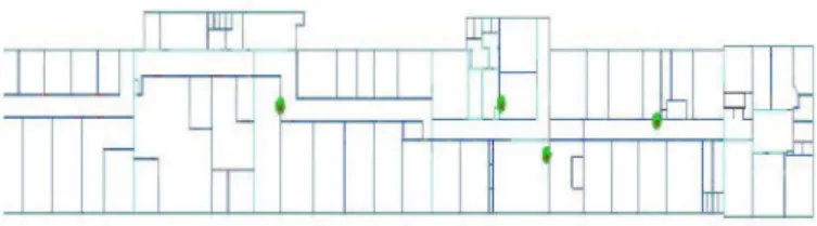
The transmitters were placed at four locations within the building. Figl shows the locations of the transmitters in the environment where the measurements were carried out.

Figure 1: Location of the transmitter antenna in the

measurements environment - (lOOmx 18.5m).

Both transmitters and receiver use an omnidrectionnal antenna. The transmitters are placed at a height of 2.5m near the ceiling (ceiling height was about of 2.88 m). The locations of reception points were at a height of 1.2m. The measurements were processed in line of sight (LOS) and non line of sight (NLOS).

Internai walls were made of 7 cm thick plasterboard with 3 cm thick wooden doors. The outer walls are made of 44 cm thick concrete with double-glazing. Floor is made of concrete. Most of the furniture is made of agglomerated wood and metallic cupboards. The building had a rectangular shape, with a S-shaped corridor separating the different rooms.

In order to remove fast fading effect, several field strength measurements, around the considered reception point, are

performed and averaged. For averaging the measurements period at each point is equal to 20s. From the 350 measured values four configurations are selected with the same number of combinations and different number of points.

The number of points par combinations increases from 2 to 5 which increase the number of points from 77 to 148.

Table 3 shows a stability of the adjusted coefficient of determination (-0.62) and the RMSE (-5.3).

The F value is always greater than the tabulated value (for a level of significance a= _{1 %, 6 variables and 60 points F}

1 %_. 6_• 60

is equal to 2.37). The F value increases statistically from 34.6 to 80 when the number of points increases from 77 to 148. The ti corresponding to the regression variables are greater than the tabulated value except for Att3 which falls bellow the

acceptable 11 %,60 =2.37 and consequently could not be

considered as influent in the regression model.

As we said in the last paragraph we can note that with only 77 points we carry out a comparable RMSE to that with 350 points (resp. 5.3 dB and 4.96 dB). With 77 points we explain 69% of path loss by regression model while we explain the same quantity with 145 points.

5 Conclusion

The calibration of propagation models is presented in many articles, but none interested in the impact of the measurement points selection on the robustness of the final result.

In this paper, statistical study of the multiple regression analysis was presented. Numerical results show that it is not an increase in the number of calibration points which increases the performances of the model. With a reduced number of points, a representative calibration points sample of the environment which provides a data matrix with better properties for parameters estimation allows a good model robustness and accuracy.

Confieuration description tj value of the model parameters [dB] Analysis

confieuration number of combination number of points loe(d) Attl Att2 Att3 Att4 cte RMSE[dB] F Ra

1 38 77 7.16 4.05 4.7 0.5 2.4 26 5.3 34.6 0.69 2 38 104 7.49 4.91 5.04 0.32 2.33 29 5.4 45.6 0.7 3 38 128 7.7 6.3 5.5 0.51 2.69 32 5.35 60 0.72 4 38 148 8.5 6.6 5.9 1.00 2.8 34 5.22 80 0.73 ail measurements 350 350 1.3 12.29 12.2 1.3 6.9 44 4.96 225 0.79

Table 3: Statistical regression analysis for four measured configurations in France telecom building (validation of the

conclusion established with simulated configurations)

References

[l] L. Chaigneaud, V. Guillet and R. Vauzelle ''A 3D ray­

tracing tool broadband wireless systems" IEEE Vehic.

Tech. Conf, Atlantic city, Oct. 2001

[2] Y. Dodge and V. Rousson ''Analyse de régression

appliquée II DUNOD, 2ème édition, 2004.

[3] J. M. Keenan and A. J. Motley "Radio coverage in

buildings" Br. Telecom. Tech. J. Vol. 8 No. 1 19-24 Jan. 1990

[4] N. Papadakis, A. Economou, J. Fotinopoulou and P. Constantinou "Radio Propagation Measurements and

Modelling of indoor Channels at 1800 MHz" Wireless Persona/ Comm.9, 95-111 1999 Kluwer Academic Publishers.

[5] A. M. D. Turkmani and A. F. de Toledo "Modelling of

radio transmission into and within multi-storey buildings at 900, 1800 and 2300MHz" IEE Proceedings-1, Vol. 140, No. 6, 462-470, Dec. 1993