HAL Id: hal-00931846
https://hal.inria.fr/hal-00931846
Submitted on 15 Jan 2014
HAL is a multi-disciplinary open access
archive for the deposit and dissemination of
sci-entific research documents, whether they are
pub-lished or not. The documents may come from
teaching and research institutions in France or
abroad, or from public or private research centers.
L’archive ouverte pluridisciplinaire HAL, est
destinée au dépôt et à la diffusion de documents
scientifiques de niveau recherche, publiés ou non,
émanant des établissements d’enseignement et de
recherche français ou étrangers, des laboratoires
publics ou privés.
Distributed Optimal Planning: an Approach by
Weighted Automata Calculus
Eric Fabre, Loïg Jezequel
To cite this version:
Eric Fabre, Loïg Jezequel. Distributed Optimal Planning: an Approach by Weighted Automata
Calculus. 48th IEEE Conference on Decision and Control, Dec 2009, Shanghai, China. pp.211-216.
�hal-00931846�
Distributed Optimal Planning:
an Approach by Weighted Automata Calculus
Eric Fabre*, Lo¨ıg Jezequel**
Abstract— We consider a distributed system modeled as a
possibly large network of automata. Planning in this system consists in selecting and organizing actions in order to reach a goal state in an optimal manner, assuming actions have a cost. To cope with the complexity of the system, we propose a distributed/modular planning approach. In each automaton or component, an agent explores local action plans that reach the local goal. The agents have to coordinate their search in order to select local plans that 1/ can be assembled into a valid global plan and 2/ ensure the optimality of this global plan. The proposed solution takes the form of a message passing algorithm, of peer-to-peer nature: no coordinator is needed. We show that local plan selections can be performed by combining operations on weighted languages, and then propose a more practical implementation in terms of weighted automata calculus.
Index Terms— factored planning, distributed planning,
op-timal planning, discrete event system, distributed constraint solving, distributed optimization, weighted automaton, K-automaton, string to weight transducer, formal language theory
I. INTRODUCTION
A planning problem [1] consists in optimally selecting and organizing a set of actions in order to reach a goal state from a given initial state. These “states” correspond to tuples
(vi)i∈I of values, one per variable Vi, i∈ I, and the actions
read and write on subsets of these variables. Expressed in these general terms, one easily guesses that a planning problem “simply” amounts to finding a path from an initial state to a (set of) goal state(s) in an automaton. In reality, the problem is more complex in several respects. First of all, the underlying automaton that encodes the problem is generally huge : the state space explodes, due to its vector nature, and actions operate on few components of the state vector, so a single action results in a huge number of transitions. There-fore, finding a path to the goal in such a huge automaton is not a trivial task and requires dedicated algorithms. Secondly, there exist planning problems of different difficulties. Some are more on the side of constraint solving: they admit few complex solutions, or even none, and one should dedicate his efforts to finding one solution, or to proving that there is no solution at all. Other problems are more accessible, in * E. Fabre is with the DistribCom team, INRIA Centre Rennes - Bretagne Atlantique, Rennes, France, [email protected]
** L. Jezequel is with ENS Cachan Bretagne, Rennes, France, [email protected]
This work was partly supported by the FAST program (Franco-Australian program for Science and Technology), Grant 18616NL, and by the European Community’s 7th Framework Programme under project DISC (DIstributed Supervisory Control of large plants), Grant Agreement INFSO-ICT-224498. This work was also supported by the joint research lab between INRIA and Alcatel-Lucent Bell Labs.
the sense that one can easily prove the existence of many solutions. The difficulty then amounts to finding the best one in an efficient manner, where “best” means that some criterion should be minimized, for example the number of actions in the plan, or the total cost of the plan, assuming each action involves some cost. The present paper addresses this second family of problems.
In order to address planning problems of growing size and complexity, several research directions have been recently explored. They essentially try to make use of the locality of actions, i.e. the fact that an action involves a small number of variables. One can for example take advantage of the concurrency of actions: when two actions are simultaneously firable and involve different sets of variables, they need not be ordered in a plan. This results in search strategies that han-dle plans as partial orders of actions rather than sequences, which reduces the search space [2], [3]. A stronger trend is known as “factored planning”, and aims at solving planning problems by parts [5], [6], [7], [8]. Formally, one can imagine that the action set is partitioned into subsets, each subset representing an “agent.” So each agent can only influence part of the resource set. The idea is then that one should build a plan for each agent, which corresponds to a smaller planning problem, and at the same time ensure that all such local plans are compatible, i.e. can be assembled to form a valid global plan. The difficulty is of course to obtain this compatibility of local plans: this is where the sparse interaction graph of agents is exploited, and where one may obtain a complexity gain.
The results presented here elaborate on this idea, but adopt a radically new perspective on the problem. Specifically, we assume that agents are sufficiently small to enable the handling of all local plans. We then focus on the
dis-tributed computations that 1/ will select local plans of each
agent that can be extended into (or that are projection of) a global plan, and 2/ will at the same time select the tuple of local plans (one per agent) that corresponds to the best global plan. As a side-product, we also obtain global plans that are partially ordered sets of actions.
Our approach first encodes the planning problem as a reachability problem in a network of automata, one automa-ton per agent (section II). We then make use of classical tools in formal language theory, distributed constraint solving [10], [11], [9], distributed optimization [13] (section III), and weighted automata calculus [16], [17] (section IV) to solve the problem. Taken separately, none of these tools is original, but their assembling certainly is, and we believe this opens a promising research direction about planning problems.
II. PLANNING IN NETWORKS OF AUTOMATA
A. From planning to distributed planning
The definition of a planning problem assumes first a finite
set of state variables {Vi}i∈I ! VI, taking values in finite
domainsDi. The initial state is a specific tuple (vi)i∈I and
we assume here a set of goal states in product form ×iGi
with Gi ⊆ Di. The second ingredient is a finite collection
of actions {ak}k∈K. An action ak usually involves a small
subset of variables V(ak) ⊆ VI. To be firable, ak must
read specific values on (some of) theV(ak), which form the
preconditions of ak. The firing of ak writes specific values
on (some of) the variablesV(ak), the so-called effect of ak.
In this paper, to avoid non-central technical complications,
we assume that each ak both reads and writes on all its
variablesV(ak). Finding an optimal plan consists in selecting
and organizing actions to go from the initial state (vi)i∈I
to one of the goal states of G = ×i∈IGi, and at the
same time minimize a criterion like the number of actions for example. This is made more formal below. Planning problems are generally expressed in different formalisms: STRIPS or PDDL assume binary variables, while SAS+ [5] or the related notion of Domain Transition Graph [4] assume multi-valued variables. Here we are closer to this second family.
To make this setting distributed, we partition the variable
set VI into subsets VIn, with $nIn = I, corresponding to
the “agents”An (one could equivalently partition the action
set). AgentAn is provided with all the actions ak restricted
to its variables VIn, ak|VIn, such thatV(ak)∩VIn &= ∅. Agent
An represents the restriction of the global planning problem
to the subset of variables VIn. Since actions are now split
into different agents, we introduce below a standard product formalism that synchronizes agents on these shared actions and allows us to recover the global planning problem from its restrictions. This way of splitting a planning problem into parts is standard and has been adopted by several “factored planning” approaches [5], [6], [7], [8], [12]. It is generally used to build global plans by parts, starting by some agent, looking for a local plan in this agent, and then trying to progressively extend it with a compatible local plan of another agent, and so on. Here, the compatibility of local plans corresponds to an agreement to jointly perform or reject some shared actions (this is formalized below).
In this paper, we adopt a different perspective. First of all, we look for a distributed planning approach and abandon the idea of a coordinator in charge of assembling the proposed local plans into a global one. We rather assume that the agents themselves are in charge of computations, relying on message exchanges, and that they only handle local information (typically sets of local plans), not global one. Secondly, rather than a search for one possible global plan (which assumes many backtrackings in the assembling of agent proposals), the method we propose is rather based on a filtering idea : it explores all local plans of an agent, and removes those that can not be the restriction of a valid global plan. Finally, beyond this filtering idea, the procedure
we propose implements as well a distributed optimization function that will compute (all) the optimal global plan(s). To our knowledge, this is the first approach to optimal factored planning.
We proceed by formalizing the notion of agent as a weighted automaton, and the notion of plan as a word in the language of this automaton.
B. Weighted automata and their languages
Let (K, ⊕, ⊗, ¯0, ¯1) denote the so-called tropical
commuta-tive semiring (R+
∪{+∞}, min, +, +∞, 0). Following [16], a weighted automaton (WA), or equivalently a string to
weight transducer, is a tupleA = (S, I, F, Σ, cI, cF, c) where
S is a finite set of states, among which I, F ⊆ S represent
initial and final states respectively, Σ is a finite alphabet
of actions, cI : I → K \ {¯0} and cF : F → K \ {¯0} are
weight/cost functions on initial and terminal states. The last
parameter c : S×Σ×S → K is a weight or cost function over
all possible transitions of A, with the convention that only
transitions in T = c−1(K\{¯0}) are possible in A (transitions
of infinite cost are impossible). Given a transition t ∈ T ,
we denote by (s−(t), σ(t), s+(t)) its three components in
S× Σ × S. A path π = t1...tn is a sequence of transitions
such that s+(t
i) = s−(ti+1), 1 ≤ i ≤ n − 1. We define
s−(π) = s−(t
1), s+(π) = s+(tn), σ(π) = σ(t1)...σ(tn)
and for the cost of this path c(π) = c(t1) ⊗ . . . ⊗ c(tn),
i.e. the sum of transition costs. The path π is accepted by
A, denoted π |= A, iff s−(π) ∈ I and s+(π) ∈ F . The
language ofA is defined as the formal power series
L(A) = !
u∈Σ∗
L(A, u) u (1)
where coefficients are given by
L(A, u) = "
π|= A u = σ(π)
cI[s−(π)] ⊗ c(π) ⊗ cF[s+(π)] (2)
L(A, u) is the weight of the action sequence (or word) u, and it is thus obtained as the minimum weight over all
accepted paths ofA that produce u, with the convention that
L(A, u) = +∞ (i.e. ¯0) when no such path exists. The word
u is said to belong to the language ofA iff L(A, u) &= ¯0.
One can associate a transition function δ : S× Σ → 2S
to A by δ(s, σ) = {s#,∃(s, σ, c, s#) ∈ T }, which extends
naturally to state sets S#⊆ S by union and to words u ∈ Σ∗
by composition. We also denote δ(s) =∪σ∈Σδ(s, σ). A is
said to be deterministic when |I| = 1 and δ is a partial
function over S× Σ, i.e. from any state s there is at most
one outgoing transition carrying a given label σ.
A WA can be considered as an encoding of a planning problem with action costs. Optimal planning then consists in finding the word(s) u of minimal weight in the language L(A), or equivalently the optimal accepted path(s) in A, which can be solved by traditional graph search. In the
se-quel, we examine the case whereA is large, but obtained by
combining smaller planning problems (called components), one per agent.
C. From distributed planning to (networks of) automata
We represent an agentAnas a WA. Its state space encodes
all possible values (vi)i∈Inon its variables, and its transitions
define how actions modify these values. Transition costs represent how much the agent must spend for a given action. The goal of agent is defined by its subset F of final states. The interaction of two agents is defined by sharing some actions, which formally takes the form of a product of WA.
Let A1,A2 be two WA, Ai = (Si, Ii, Fi, Σi, cIi, cFi, ci)
with Tias associated transition sets, their productA = A1×
A2= (S, I, F, Σ, cI, cF, c) is defined by S = S1× S2, I =
I1× I2, F = F1× F2, Σ = Σ1∪ Σ2, cI = cI1◦ p1⊗ cI2◦
p2, cF = cF1◦ p1⊗ cF2◦ p2 where the pi: S1× S2→ Si
denote the canonical projections. For transition costs, one has c((s1, s2), σ, (s#1, s#2)) = c1(s1, σ, s#1) ⊗ c2(s2, σ, s#2) if σ ∈ Σ1∩ Σ2 c1(s1, σ, s#1) if σ &∈ Σ2 and s2= s#2 c2(s2, σ, s#2) if σ &∈ Σ1 and s1= s#1 ¯0 otherwise (3)
The first line corresponds to synchronized actions : the two
agents must agree to perform shared actions of Σ1∩ Σ2,
in which case action costs are added. By contrast, actions carrying a private label remain in the product as private actions, where only one agent changes state (next two lines). We now model a distributed planning problem as a product
A = A1× ... × AN, which can be seen as a network of
interacting agents. The objective is to find the/a path π from
I = I1× ... × In to the global objective F = F1× ... × FN
that has minimal cost inA. Equivalently, we look for a word
u in the language of A that has minimal weight L(A, u).
We will actually look for an N -tuple of words (u1, ..., uN),
one word ui per componentAi, where each ui corresponds
to the canonical projection of u on (the action alphabet of)
agent Ai. Such local paths πi are said to be compatible.
The next section explains how to compute an optimal tuple of compatible local plans without computing optimal global plans.
III. DISTRIBUTED OPTIMAL PLANNING BY(WEIGHTED)
LANGUAGE CALCULUS
A. Basic operations on weighted languages
Let us first define the product of weighted languages
(WL). For a word u ∈ Σ∗ and Σ# ⊆ Σ, we denote by
u|Σ" the natural projection of u on the sub-alphabet Σ#. Let
L1,L2be two WL defined as formal power series on Σ1, Σ2
respectively, their product is given by
(L1×LL2)(u) = L1(u|Σ1) ⊗ L2(u|Σ2) (4)
Proposition 1: ForA = A1× ... × AN one hasL(A) =
L(A1) ×L...×LL(AN).
Proof: The result is well known if weights are
ig-nored [10], [14]. Regarding weights, let us consider the case of two components, without loss of generality. Let
u ∈ (Σ1∪ Σ2)∗ such that its projections ui = u|Σi have
non vanishing costs : L(Ai, ui) &= ¯0. Let πi be an accepted
path inAi such that σi(πi) = ui. By definition ofA1× A2,
one can interleave π1 and π2 into a path π |= A such that
σ(π) = u. Conversely, let π|= A such that σ(π) = u. Since
transitions of A are pairs of transitions of A1 andA2, the
canonical restriction of π to theAi part yields a πi |= Ai
such that σi(πi) = ui. As a consequence, the⊕ in (2) splits
into a product of two sums, one for each component, which
yieldsL(A, u) = L(A1, u1) ⊗ L(A2, u2).
The second operation we need is the projection of a WL
L defined on alphabet Σ on a subset Σ# ⊆ Σ of action
labels. As for regular languages, this amounts to removing the non desired labels, but here we combine it with a cost optimization operation over the discarded labels :
∀u#∈ Σ#∗, Π
Σ"(L)(u#) =
" u∈Σ∗, u|Σ"=u"
L(u) (5)
Proposition 2: Let u be an optimal word ofL, i.e. L(u) = '
v∈Σ∗L(v), then u# = u|Σ" is an optimal word of L# =
ΠΣ"(L), i.e. L#(u#) = 'v"∈Σ"∗L#(v#). And conversely, an
optimal word u# of L# is necessarily the projection on Σ# of
an optimal word u ofL.
Proof: Direct consequence of (5).
Proposition 2 has an important meaning for distributed
planning. Consider the set of global plans L(A) and its
projections ΠΣi(L(A)) on the action sets of all components.
Then an optimal local plan ui in ΠΣi(L(A)) is necessarily
the projection of an optimal global plan u ∈ L(A) : ui =
u|Σi. And the latter induces optimal local plans uj = u|Σj
in all the other projected languages ΠΣj(L(A)), j &= i.
Moreover, if the optimal local plan ui is unique in every
ΠΣi(L(A)), then these local plans are necessarily the
pro-jection of the same u, i.e. they are compatible (by definition). In summary, our objective is to compute the projections
ΠΣi(L(A)) on the action alphabets of components Ai, and
then select the optimal words in these local languages. It turns out that these projected languages can be obtained
without computing L(A), as we show below. B. Distributed planning
Theorem 1: LetL1,L2 be weighted languages on Σ1, Σ2
respectively, and let Σ1∩ Σ2⊆ Σ#, then
ΠΣ"(L1∧ L2) = ΠΣ"(L1) ∧ ΠΣ"(L2) (6)
Proof: Again, the result is standard on languages when
weights are ignored [9]. To take weights into account, assume
for simplicity that Σ#= Σ
1∩Σ2. The proof is then similar to
the one of Prop. 1 : for any two words ui∈ Li, i = 1, 2, such
that u1|Σ" = u2|Σ", one will have a joint word u inL1∧ L2,
and vice-versa. It is then sufficient to notice that in (6) the
sum⊕ that removes the extra labels of (Σ1∪ Σ2)\Σ# in the
left-hand side projection can be split into a product of two
independent sums, one removing labels of Σ1\Σ# in the u1
terms, and another one removing labels of Σ2\Σ# in the u2
terms. This gives the right-hand side of (6).
Theorem 1 is central to derive distributed constraint solv-ing methods [12] (useful here to select compatibles local
plans), as well as distributed optimization methods [13] (useful here to derive the local views of optimal global plans). These approaches are actually two facets of a more general theory developed in [9]. We combine them here to design a distributed method for optimal planning. For a matter of simplicity, we illustrate the concepts on a simple example.
Consider a planning problem defined asA = A1×A2×A3
whereAi is defined on the action alphabet Σiand such that
Σ1∩ Σ3⊆ Σ2. This assumption states that every interaction
ofA1andA3 involvesA2, or equivalently thatA1 andA3
have conditionally independent behaviors given a behavior of
A2. One can graphically represent this assumption by means
of an interaction graph (Fig. 1). An interaction graph has
componentsAi as nodes; edges are obtained by recursively
removing redundant edges, starting from the complete graph.
The edge (Ai,Aj) is declared redundant iff either Σi∩Σj =
∅, or it is included in every Σk along an alternate path from
Ai toAj in the (remaining) graph.
1
A
2A
3A
Fig. 1. The interaction graph ofA = A1×A2×A3when Σ1∩Σ3⊆ Σ2.
Consider the derivation of ΠΣ1[L(A)]. From
Proposi-tion 1, one hasL(A) = L(A1) ×LL(A2) ×LL(A3). Then
ΠΣ1[L(A)]
= ΠΣ1[ L(A1) ×LL(A2) ×LL(A3) ]
= L(A1) ×LΠΣ1[ L(A2) ×LL(A3) ]
= L(A1) ×LΠΣ1∩Σ2[ L(A2) ×LL(A3) ]
= L(A1) ×LΠΣ1∩Σ2[ L(A2) ×LΠΣ2∩Σ3[L(A3)] ] (7)
The second equality uses Theorem 1 with Σ# = Σ
1 ⊇
Σ1∩ (Σ2∪ Σ3), and the fact that ΠΣ1[L(A1)] = L(A1).
For the third equality, observe that languageL = L(A2) ×L
L(A3) is defined on the alphabet Σ2∪ Σ3. So ΠΣ1(L) =
ΠΣ1[ΠΣ2∪Σ3(L)] = ΠΣ1∩(Σ2∪Σ3)(L). This is where our
assumption comes into play to obtain Σ1∩ (Σ2∪ Σ3) =
Σ1∩ Σ2. For the fourth equality, one replaces first ΠΣ1∩Σ2
by ΠΣ1∩Σ2◦ΠΣ2. The derivation of ΠΣ2[L(A2)×LL(A3)] =
L(A2) ×L ΠΣ2∩Σ3[L(A3)] is again a direct application
of Theorem 1, and reproduces the derivation of the third equality.
Equation (7) reveals that the desired projection ΠΣ1[L(A)]
can be obtained by a message passing procedure, following
the edges of the interaction graph. The message fromA3 to
A2 is ΠΣ2∩Σ3[L(A3)]. It is combined with the knowledge
ofA2 and the result is projected on Σ1∩ Σ2to produce the
message fromA2 toA1. A symmetric message propagation
rule would yield ΠΣ3[L(A)], and one can also prove that
ΠΣ2[L(A)]
= ΠΣ1∩Σ2[L(A1)] ×LL(A2) ×LΠΣ2∩Σ3[L(A3)] (8)
So the two incoming messages at A2 are sufficient to
compute ΠΣ2[L(A)]. The interest of this message passing
strategy is triple: the procedure is fully distributed (no coordinator is needed), it only involves local information, and it has low complexity, in the sense that only two messages per edge are necessary (one in each direction). While the product generally increases the size of objects, one can expect the projection to reduce it, and thus save in complexity (this still has to be quantified more precisely, however).
A full theory allows one to extend this simple example to systems which interaction graph is a tree (and beyond, with more complications) [9]. C. Example !!" "!# "!" #!# c,1 !!" !!# 3
A
d,5 !!# b,0 a,1 "!" #!"A
1A
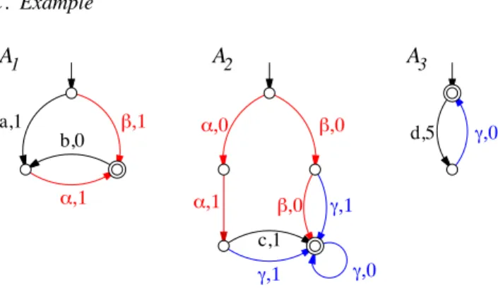
2 #!#Fig. 2. A network of 3 interacting weighted automata.
Consider the distributed system A = A1 × A2 × A3
where the three componentsAi are WA depicted in Fig. 2
(assuming cI = cF = 0). A1 andA2 share actions {α, β},
and A2,A3 share action {γ}, which corresponds to the
ineraction graph in Fig. 1. One hasL(A1) = 1 · β + 2 · aα +
2 ·βbα+3·aαbα+..., L(A2) = 0 ·ββγ∗+ 1 ·βγγ∗+ ... and
L(A3) = (n≥0n· (dγ)n. Observe that the minimal words
in these language are β, ββγ∗ and ', respecively, and that
they are not compatible.
Let us follow (7) to compute ΠΣ3[L(A)]. The message
sent by A1 to A2 is Π{α,β}[L(A1)] = 1 · β +(n≥1(1 +
n)· (' + β)αn, which will kill all solutions with two β in
L(A2): at most one β can be performed in A1. Specifically,
composed with L(A2) this message yields 2 · βγγ∗ + 5 ·
αα(c + γ)γ∗, which is also Π
Σ2[L(A1) ×LL(A2)], i.e. the
vision fromA2of whatA1andA2 can perform together to
reach their goals. Projected on γ, this yields 2· γγ∗+ 5 · ',
the message fromA2 toA3. Observe that the 5· γγ∗part is
discarded by the optimization step. Finally, composing this
message withL(A3) yields the desired ΠΣ3[L(A)] = 5 · ' +
(
n≥0(7 + 5n) · (dγ)n+1. This reveals (Proposition 2) that
the best plans or words inL(A) have cost 5, and require A3
to do... nothing!
Following exactly (7) and (8) yields the other projections
ΠΣ1[L(A)] = 5·aαbα+ 7 ·β and ΠΣ2[L(A)] =
(
n≥0[(5 +
5n) · α2c + (7 + 5n)
· βγ + (10 + 5n) · α2γ]γn. The minimal
word in each Πi[L(A)] is unique, and all of them have
cost 5, which yields the triple (aαbα, α2c, ') as an optimal
(factored) plan of cost 5. These three words are of course
compatible. Notice that component A1 has to go twice
through its local goal to help A2 and A3 reach their own
IV. IMPLEMENTATION INTO WEIGHTED AUTOMATA CALCULUS
A. Recoding primitive operations
Languages of WA are generally infinite objects, so they can not be handled as such in practice. Fortunately, one
starts computations with the regular languages L(Ai), and
the two primitive operations product×L and projection Π.
both preserve the regularity. Therefore one possibility to perform the distributed computations of section III is to replace every regular language by its finite representation as a WA. Specifically, one can choose to represent every regular language by its minimal deterministic weighted automaton (MDWA), provided it exists. The minimality is interesting to reduce the complexity of products and projections, and minimality is well defined for deterministic WA. Dealing with deterministic automata reduces as well the complexity of basic operations. But it has another important advantage for optimal planning applications: there is only one path representing a given word of the language, therefore all sub-optimal (and thus useless) paths for this word are removed in the determinization step.
Consider two minimal deterministic WA A and A#. The
product of their languagesL(A)×LL(A#) can be represented
by M in(A ×A#). One already has L(A ×A#) = L(A) ×
L
L(A#) by Proposition 1, and A × A#is deterministic.
There-fore only a minimization step (M in) is necessary, and there exist polynomial minimization algorithms for deterministic WA (not described here for a matter of space):One proceeds with a generic weight pushing procedure, followed by a standard minimization step [17].
Difficulties appear with the projection. Let A be a
de-terministic WA on alphabet Σ, its projection on Σ# ⊆ Σ
is obtained as for non-weighted automata, by first perform-ing an epsilon-reduction, then determinizperform-ing the result. The epsilon-reduction collapses all transitions labeled by Σ” =
Σ\Σ#. Specifically, one obtainsA# = (S, I#, F#, Σ#, c#
I, c#F, c#)
where the new transition function c# satisfies
c#(s, σ#, s#) = "
π : s−(π) = s, s+(π) = s" σ(π)∈ σ"Σ”∗
c(π) (9)
The initial and final cost functions are modified in a similar manner; again we refer the reader to [17] for details.
a,1 c,0 c,0 b,1 a,0 b,0
Fig. 3. A weighted automatonA that can not be determinized. The true difficulty lies in the determinization step : not all
weighted automata can be determinized. A counter-example
is provided in Fig. 3. The point is that in a deterministic WA, a unique path (and therefore a unique and minimal
weight) is associated to any accepted sequence of Σ∗. In
A, the accepted sequences are c{a, b}∗, and one either
pays for the a or for the b, according to the path selected for the first c. The weight of an accepted sequence w is
thus min(|w|a,|w|b). Intuitively, a deterministic automaton
recognizing this language must count the a and the b in order to determine the weight of a word. And so it can not be finite. A sufficient conditionfor determinizability is the so-called twin property:
Definition 1: InA, two states s, s#∈ S are twins iff, either
!u ∈ Σ∗such that s, s#∈ δ(I, u), i.e. they can not be reached
by the same label sequence from the initial states, or∀u ∈
Σ∗ : s ∈ δ(s, u), s#∈ δ(s#, u), one has
" π, σ(π) = u s−(π) = s+(π) = s c(π) = " π", σ(π") = u s−(π") = s+(π") = s" c(π#)
A has the twin property iff all pairs of states are twins.
In other words, when states s, s# can be reached by the
same label sequence, if it is possible to loop around s and
around s# with the same label sequence u, then these loops
must have identical weights.
The twin property can be tested in polynomial time [16]. It is clearly preserved by product, but unfortunately not by projection. See the counter-example above (Fig. 3) where
one of the (c, 0) would be a (d, 0). ThenA would have the
twin property. But after projection on{a, b} the property is
obviously lost. Therefore, in order to perform computations on WA, we have to assume that the twin property is preserved
by all projections. Otherwise there is no guarantee that the
determinization procedure would terminate. Notice however that, strictly speaking, this is not an obstacle to computations since the latter can be performed with any compact represen-tative of a given WL. In an extended version of this work, we show how to get rid of the twin property by a partial determinization.
The determinization procedure of a WA A elaborates on
the classical subset construction for the determinization of standard automata, which may have an exponential
complex-ity. For u∈ Σ∗ and s∈ S, let us define
C(u, s) = "
π : σ(π) = u, s−(π)∈ I, s+(π) = s
cI(s−(π)) ⊗ c(π), (10)
and C(u) = 's∈SC(u, s). So C(u, s) is the minimal
weight among paths that start in I, terminate in s and
produce the label sequence u. States of Det(A) take the
form q = (A, λ) where A ⊆ S is a subset of states, and
λ : A→ R+\{¯0}. The initial state of Det(A) is q
0= (I, λ0)
with λ0(s) = C(', s)4C(') = C(', s)−C('). Given u ∈ Σ∗
accepted byA, the unique state q = (A, λ) reached by u in
Det(A) is such that : A = δ(I, u), as usual, and one has
λ(s) = C(u, s)4 C(u) = C(u, s) − C(u). So λ(s) is the
(positive) residual over the best cost to produce u when one wants also to terminate in s. There is an obvious recursion
determining the new state q# = (A#, λ#) obtained by firing
the complete details of the algorithm, and for a termination proof when the twin property is satisfied.
B. Example
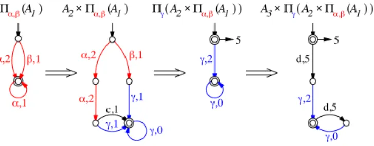
Let us reconsider the example in Fig. 2. Fig. 4 illustrates
the propagation of messages from A1 to A3, that was
described in terms of language computations in section III-C.
Observe that the message from A2 toA3 (3rd automaton)
now has a termination cost of 5 at the initial state. This
corresponds to the path α2c, that yields the empty string
' after projection on label γ. The rightmost automaton
corresponds to ΠΣ3[L(A)]. Its optimal path to a terminal
state is the empty string and has cost 5, the cost of an optimal global plan. !!$ A3 A1 !!# 5 A2 !!$ d,5 !!# "!$ #!" "!" A1 !!# c,1 !!" !!" #!" "!$ A2 A1 d,5 A1 A2 5 "!$ $%&%%%%%%%%%%%%%%%%%%%%%%' "!#
$%%%%&%%%%' $%%%%&%%%%'"!# $%&%%%%%%%%%%%%%%%%%%%%%%'! $%%%%&%%%%'"!# ! $%%%%&%%%%'"!#
Fig. 4. Propagation of messages fromA1toA3.
Performing (7) and (8) in terms of WA computations completes the derivation of the MDWA representing the
projected languages ΠΣi[L(A)] (Fig. 5). The optimal path in
each of them appears in bold lines. These paths are unique, are associated to the same optimal cost of 5 (Proposition 2), and yield the triple (aαbα, ααc, ') as best factored plan.
"!$ A c d A a,1 !!$ #!" 5 6 "!" b,0 A "!$ a,b 1 d,5 d,5 !!# "!$ !!( !!) !!( c,1 #!" "!#!
$%%%%%%%%%%&%%%' $%%%%%%%%%%&%%%'"!#!!! $%%%%%&%%%'!!
Fig. 5. The 3 MDWA representing the projected languages ΠΣi[L(A)].
V. CONCLUSION
We have described a distributed optimal planning proce-dure, based on a message passing strategy and on weighted automata calculus. To our knowledge, this is the first ap-proach combining distributed planning to distributed op-timization. The standpoint adopted here is unusual with respect to the planning literature, in the sense that one does not look for a single solution, but for all (optimal) solutions. This is made possible by several ingredients: working at the scale of small components makes computations tractable, looking for plans as tuples of local plans introduces a partial order semantics that implicitly reduces the trajectory space,
and finally representing the trajectory space as a product of local trajectory spaces is generally more compact.
The limitations we have mentioned, namely the potential exponential complexity of determinization, and the possi-bility that determinization could not be possible at all, can easily be overcome. First of all because there is no necessity to perform computations with the minimal deterministic WA representing a weighted language : Any compact rep-resentative of this language can be used. Secondly, when determinization is not possible, one can perform a partial determinization (that will be described in an extended version of this work). Another controversial aspect may be that we aim at all solutions, which may be impractical in some cases. Again, classical approximations (handling subsets of the most promising plans for example) can be designed. We are currently working on these aspects, on a detailed complexity analysis and on the validation of this approach on classical benchmarks.
Acknowledgement : The authors would like to thank Philippe Darondeau for fruitful discussions about this work.
REFERENCES
[1] Dana Nau, Malik Ghallab, Paolo Traverso, “Automated Planning: Theory & Practice,” Morgan Kaufmann Publishers Inc.,San Francisco, CA, USA, 2004.
[2] Sarah Hickmott, Jussi Rintanen, Sylvie Thiebaux, Lang White, “Plan-ning via Petri Net Unfolding,” in Proc. of the 20th Int. Joint Conf. on Artificial Intelligence (IJCAI-07).
[3] B. Bonet, P. Haslum, S. Hickmott, S. Thiebaux, “Directed Unfolding of Petri Nets,” in Proc. of the Workshop on Unfolding and Partial Ordered Techniques (UFO-07), associated to 28th Int. Conf. on Application and Theory of Petri Nets and Other Models of Concurrency, 2007. [4] Yixin Chen, Ruoyun Huang, Weixiong Zhang, “Fast Planning by
Search in Domain Transition Graphs,” AAAI-08, 23rd Conference on Artificial Intelligence, 2008.
[5] Ronen I. Brafman, Carmel Domshlak, “Factored Planning: How, When, and When Not,” AAAI-06, 21st Conference on Artificial Intelligence, Boston, MS, August 2006.
[6] Ronen I. Brafman, Carmel Domshlak, “From One to Many: Planning for Loosely Coupled Multi-Agent Systems,” ICAPS-08, 18th Interna-tional Conference on Automated Planning and Scheduling, Sydney, Australia, September 2008.
[7] Eyal Amir, B. Engelhardt, “Factored Planning,” 18th Int. Joint Con-ference on Artificial Intelligence (IJCAI’03), 2003.
[8] Jaesik Choi, Eyal Amir, “Factored planning for controlling a robotic arm: theory,” 5th Int. Cognitive Robotics workshop (CogRob 2006), 2006.
[9] E. Fabre, “Convergence of the turbo algorithm for systems defined by local constraints,” INRIA research report no. PI 4860, May 2003. [10] R. Su, W.M. Wonham, J. Kurien, X. Koutsoukos, “Distributed
Diag-nosis for Qualitative Systems,” in Proc. 6th Int. Workshop on Discrete Event Systems, WODES02, pp. 169-174, 2002.
[11] Rong Su, “Distributed Diagnosis for Discrete-Event Systems,” PhD Thesis, Dept. of Elec. and Comp. Eng., Univ. of Toronto, June 2004. [12] Rina Dechter, “Constraint Processing,” Morgan Kaufmann, 2003. [13] Judea Pearl, “Fusion, Propagation, and Structuring in Belief
Net-works,” Artificial Intelligence, vol. 29, pp. 241-288, 1986.
[14] C. Cassandras, S. Lafortune, “Introduction to Discrete Event Systems,” Kluwer Academic Publishers, 1999.
[15] J. Berstel, “Transductions and Context-Free Languages,” Electronic Edition, May 2007.
[16] Mehryar Mohri, “Finite-State Transducers in Language and Speech Processing,” Computational Linguistics, 23:2, 1997.
[17] Mehryar Mohri, “Weighted automata algorithms,” In Werner Kuich and Heiko Vogler, editors, Handbook of weighted automata. Springer (to appear), 2009.