Automated medical scheduling : fairness and quality

Automated Medical Scheduling: Fairness and Quality

Thèse

Émilie Picard-Cantin

Doctorat en informatique

Philosophiæ doctor (Ph. D.)

Québec, Canada

Automated Medical Scheduling :

Fairness and Quality

Thèse

Émilie Picard-Cantin

Sous la direction de:

Claude-Guy Quimper, directeur de recherche Mathieu Bouchard, codirecteur de recherche

Résumé

Dans cette thèse, nous étudions les façons de tenir compte de la qualité et de l’équité dans les algorithmes de confection automatique d’horaires de travail. Nous découpons ce problème en deux parties.

La modélisation d’un problème d’horaires permet de créer des horaires plus rapidement qu’un humain peut le faire manuellement, puisqu’un ordinateur peut évaluer plusieurs horaires simultanément et donc prendre des décisions en moins de temps. La première partie du problème étudié consiste à améliorer la qualité des horaires en encodant des contraintes et des préférences à l’aide de modèles mathématiques. De plus, puisque la création est plus rapide à l’aide d’un ordinateur, il est plus facile pour un ordinateur de trouver l’horaire ayant la meilleure qualité lorsque les règles et préférences sont clairement définies.

Toutefois, déterminer les règles et préférences d’un groupe de personne n’est pas une tâche facile. Ces individus ont souvent de la difficulté à exprimer formellement leurs besoins et leurs préférences. Par conséquent, la création d’un bon modèle mathématique peut prendre beaucoup de temps, et cela même pour un expert en création d’horaires de travail. C’est pourquoi la deuxième partie de cette thèse concerne la réduction du temps de modélisation à l’aide d’algorithmes capable d’apprendre un modèle mathématique à partir de solutions données comme par exemple, dans notre cas, des horaires de travail.

Abstract

In this thesis, we study the ways to take quality and fairness into account in the algorithms of automatic creation of work schedules. We separate this problem into two subproblems. The modeling of a scheduling problem allows a faster creation of schedules than what a human can produce manually. A computer can generate and evaluate multiple schedules at a time and therefore make decisions in less time. This first part of the studied problem consists in improving the quality of medical schedules by encoding constraints and preferences using mathematical models. Moreover, since the creation is faster, it is easier for a computer to find the schedule with the highest quality when the rules and the preferences are clearly defined. However, determining the rules and preferences of a group of people is not an easy task. Those individuals often have difficulties formally expressing their requirements and preferences. Therefore, the creation a good mathematical model might take a long time, even for a scheduling expert. This is why the second part of this thesis concerns the reduction of modeling time using algorithms able to learn mathematical models from given solutions, in our case schedules.

Contents

Résumé iii

Abstract iv

Contents v

List of Tables vii

List of Figures viii

Remerciements xi

Introduction 1

1 Medical Scheduling: The Problem 3

1.1 What is a medical schedule? . . . 3

1.2 Industrial context . . . 4

1.3 The importance of automated scheduling . . . 7

1.4 Related problems . . . 8

1.5 Balancing a schedule . . . 10

1.6 Other balancing problems . . . 13

1.7 Other constraint acquisition problems . . . 14

2 Combinatorial Optimization 17 2.1 Constraint Programming . . . 18

2.2 Mixed integer programming . . . 29

2.3 Flow networks . . . 34

2.4 Markov chains . . . 37

3 The Balance Constraint Family 38 3.1 Introduction . . . 38

3.2 The constraints . . . 39

3.3 The complexity of achieving domain consistency . . . 40

3.4 Decompositions . . . 45

3.5 A filtering algorithm for AtMostBalance* . . . 55

3.6 Application to the Balanced Academic Curriculum Problem . . . 64

3.7 Application to the Shift Scheduling Problem . . . 67

4 Distribution of events in a Cyclic Schedule 71

4.1 Introduction . . . 72

4.2 Distribution metric . . . 74

4.3 Two linear optimization models . . . 76

4.4 Application to the Shift Scheduling Problem . . . 82

4.5 Application to the Car Sequencing Problem . . . 87

4.6 Discussion . . . 90 4.7 Conclusion . . . 91 5 Constraint Acquisition 92 5.1 Introduction . . . 93 5.2 Listing Candidates . . . 95 5.3 Probabilities . . . 96 5.4 Constraint Dominance . . . 100 5.5 Classifier . . . 101 5.6 Soft Constraints . . . 102 5.7 Branch-and-bound . . . 105 5.8 Monotonicity . . . 106

5.9 Bounding and filtering specific constraints . . . 108

5.10 Comparing brute force statistical and solution counting algorithms . . . 113

5.11 Comparing branch-and-bound and brute force statistical algorithms . . . 117

5.12 Conclusion . . . 122

Conclusion 124

List of Tables

2.1 Domain consistency applied to a small set of constraints . . . 21

2.2 Example of an unbalanced schedule . . . 24

3.1 Example of a medical schedule for a single physician where two out of three tasks are assigned. . . 39

3.2 Summary of the complexities for the filtering algorithms of the balancing constraints . . . 45

3.3 Balanced Academic Curriculum Problem . . . 67

3.4 Results for the shift scheduling problem. . . 70

4.1 Percentage of solutions of each type for each model. . . 86

4.2 Percentage of instances for each type of solution and each model for the Car Sequencing problem with 100 cars . . . 89

4.3 Percentage of instances for each type of solution and each model for the Car Sequencing problem with 200 cars . . . 89

4.4 Percentage of instances for each type of solution and each model for the Car Sequencing problem with 25 cars . . . 90

5.1 Results for Counting and Statistical with a single positive example by instance . . . 117

5.2 Results for SubsetFocus. Number of instances for which the initial constraint was ranked first, second, third or was not found. . . 121

5.3 Results for Sequence. Number of instances for which the initial set of parameters was ranked first, second, third or was not found. . . 123

List of Figures

1.1 Two representations of the same schedule with 3 employees and 2 tasks (day

and night shifts) . . . 4

1.2 Two different scenarios for the distribution of workloads among three physicians over a scheduling horizon of four days. . . 11

1.3 Two different scenarios for the distribution of task types for a physician over a scheduling horizon of four days. . . 11

1.4 Two different scenarios for the same physician with two tasks, emergency room and surgery. . . 12

1.5 Each pattern is repeated once showing the effect of repeating a poorly distributed pattern. . . 12

1.6 Two scenarios with different spacings. The first schedule has one spacing of length 2 and one of length 0. The second schedule has two spacings of length 1. 12 2.1 Different versions of a search tree depending on branching order and if filtering is applied. . . 20

2.2 Automaton A . . . 25

2.3 Unfolded version of the automaton of Example 4 for sequences of n = 6 characters. 27 2.4 Automaton corresponding to Sequence([Y1, . . . , Yn], 1, 1, 3, [0, 1]) . . . 28

2.5 Representation of the problem A ~X = ~b when separating matrix A into two submatrices . . . 33

2.6 Simple directed graph with a source s, a sink σ and two nodes n1 and n2. . . . 34

2.7 Same directed graph as Figure 2.6 with capacities. . . 35

2.8 Residual network corresponding to the flow in Figure 2.7. The arc (n1, σ) has been split into two arcs since the initial capacity was not used fully. We can still push two units of flow on the arc or we can take back the one unit that has been pushed already. . . 36

3.1 Automaton for Decomposition 5 . . . 52

3.2 Graph G for the constraint AtMostBalance*([X1, X2, X3, X4], B, V = {1, 2}) with arc capacities. . . 57

3.3 Residual graph G0 _{after applying the maximum flow on graph G. . . . 58}

3.4 Residual graph G00 _{after applying the modifying path on the residual graph G}0_{. 58} 3.5 Standard model . . . 65

3.6 AtMostBalance* model . . . 65

3.7 Deviation model . . . 66

3.8 GCC +Deviation model . . . 66

3.10 Decomposition 3 model for the shift scheduling problem . . . 68

3.11 Decomposition 4 model for the shift scheduling problem . . . 69

3.12 AtMostBalance* model for the shift scheduling problem . . . 69

4.1 Typical medical schedule for four days, two tasks and two physicians. . . 73

4.2 Boolean schedule for one of the two physicians of Figure 4.1, all tasks considered. A dark box means the physician is assigned to at least one task for the day. . 73

4.3 Scenarios for a 4-day cyclic schedule with two worked days and two days off. Scenario A consist of two consecutive worked days and Scenario B alternates between worked days and days off. . . 74

4.4 Each pattern is repeated three times showing the cycling effect of repeating a poorly distributed pattern. . . 74

4.5 The quality of an individual spacing of length bij is given by this partially quadratic function. The penalty for a spacing smaller then the threshold L is always maximum and a spacing larger then the ideal length Im is not penalized. 75 4.6 Complete graph for scenario B of Figure 4.3 where thicker arcs represent the flow circulating in the graph. We have Λ1 = Λ3 = 1, Λ2= Λ4= 0, y13= y31= 1 and yij = 0 otherwise. . . 76

4.7 Multiple sub-graphs optimization model for the distribution of worked days over the scheduling period. . . 77

4.8 Single graph optimization model for the distribution of worked days over the scheduling period. . . 80

4.9 Time comparison between M and S for the scheduling problem. The largest confidence interval observed on resolution time for these instances is ±52 seconds, 99% of the time. . . 86

4.10 Objective value comparison between M and S for the scheduling instances. The worst confidence interval observed on objective value for these instances is ±0.003, 99% of the time. . . 87

4.11 Complete distribution model for the Car Sequencing problem. . . 88

4.12 Time comparison between M and S for the Car Sequencing instances (25 cars). The worst confidence interval observed on resolution time for these instances is ±80 seconds, 99% of the time. . . 90

4.13 Objective value comparison between M and S for the Car Sequencing instances (25 cars). The worst confidence interval observed on objective value for these instances is ±0.005 , 99% of the time. . . 91

5.1 Task-oriented schedule . . . 93

5.2 Markov chain for Sequence([X1, . . . , Xn], 1, 2, 3, ~z = [0, 1]) when p0 = 5/6and p1 = 1/6. The state σ is reached when reading a sequence that violates the constraint Sequence. The transitions are labeled "characted read: transition probability". . . 99

5.3 Visual representation of dominance for the Sequence constraint. . . 101

5.4 Graphical representation of the Markov chain corresponding to the hard constraint Sequence([X1, . . . , Xn], 0, 1, 3, ~z = [0, 1]) with p0 = 5/6 and p1 = 1/6. The transitions are labeled "characted read: transition probability". . . . 103

5.5 Markov chain for SoftSequence([X1, . . . , Xn], V, 0, 1, 3, ~z = [0, 1]) when p0 =

5/6and p1 = 1/6. The transitions leading to new violations are split into two

arcs: the portion of considered violations (β) and the portion of non-considered violations (1 − β). The transitions are labeled "characted read: transition

probability". . . 104 5.6 Number of incorrectly classified instances in percentage for each method and

each number of examples . . . 118 5.7 Number of incorrectly classified instances in percentage after false negatives

have been removed . . . 118 5.8 Comparison between the branch-and-bound and the brute force for learning

parameters of SubsetFocus. . . 120 5.9 Comparison between the branch-and-bound and the brute force for learning

Remerciements

Bien que le doctorat soit le travail de l’étudiant gradué, la recherche doctorale et la rédaction de la thèse est rarement accessible sans appui ni soutien. Je ne compte pas les heures que j’ai mises sur cette thèse, puisque ce serait probablement démoralisant, toutefois je ne suis pas la seule à avoir consacré du temps à ce projet de recherche. J’aimerais remercier dans cette section les gens sans qui cette thèse n’existerait pas aujourd’hui.

Merci à PetalMD notre partenaire industriel, tout particulièrement Jason Pierre Sweeney et François-Pierre Bouchard, de m’avoir donné la chance de travailler sur un projet concret et passionnant. Cette collaboration m’aura permis non seulement d’apprendre sur l’optimisation des horaires de travail mais également d’acquérir de l’expérience en entreprise lors de mes études.

Merci à mon directeur de recherche, Claude-Guy Quimper. Tu étais là chaque fois que j’en avais besoin, que ce soit pour répondre à mes questions ou m’encourager lorsque je manquais de motivation. Tu as toujours eu une passion pour notre projet, même quand je doutais de l’importance de nos résultats. Merci d’avoir collaboré avec moi pendant toutes ces années et de toujours avoir accordé de l’importance à mon opinion. Dès la première rencontre, je me suis sentie comme ta collègue et non seulement une étudiante. Merci de m’avoir donné la chance de voyager et d’aller présenter nos résultats de recherche à l’international. Finalement, merci d’être un directeur de recherche incroyable. Je crois que peu d’étudiants ont la chance de travailler avec quelqu’un comme toi durant leurs études et je te remercie d’avoir cru en moi dès le départ et d’avoir misé sur notre projet.

Merci à mon co-directeur et collègue, Mathieu Bouchard. Il n’est pas facile d’arriver dans une équipe et d’avoir le tac de ne pas écraser d’orteils tout en se faisant une place. Merci pour ta patience quand tu m’expliquais de nouveaux concepts que je n’arrivais pas à saisir. Merci d’avoir consacré de ton temps personnel à notre projet au fil des années. Merci d’avoir été un ambassadeur pour notre projet au sein de l’entreprise lorsque je ne pouvais pas l’être. Finalement, merci d’être un collègue formidable avec qui j’ai pu faire des boutades et avoir des fous rires. Ce fut un réel plaisir de travailler avec toi.

Beldiceanu, d’avoir pris le temps de lire ma thèse. Merci également pour l’intérêt marqué que vous avez porté à mon projet de recherche. J’ai beaucoup apprécié discuter avec vous de mon projet.

Merci à mon conjoint, Alexandre Guay-Langlois, d’avoir partagé avec moi toutes mes victoires et tous mes échecs. Je ne serais pas là où j’en suis aujourd’hui sans ton dévouement et ta patience.

Introduction

Medical professionals or physicians occupy different types of tasks such as surgery, emergency room tasks, patient consultation, on call, etc. Medical tasks are important and some require to be covered 24 hours a day, 365 days a year. Creating schedules for physicians is crucial to maintaining a high quality service of health care providers. However, those schedules should satisfy administrative rules, such as the maximum number of hours per day per person, and physicians’ availability. The best schedules also satisfy physicians’ preferences on assignment as much as possible. Physicians are grouped together for scheduling, either by hospital or by specialty. The manager of each group is in charge of creating the working schedules. This administrative task can take hours to accomplish. This physician’s time could be better used helping patients.

For this reason, PetalMD was founded in 2009 with the main goal of lightening administrative tasks for physicians. Their motto: Put the focus back on what matters most : patients.1

One of PetalMD’s product, PetalScheduling, allow the creation of schedules. It also allows physicians of a group to access their schedule at any time from multiple devices and trade tasks with other physicians. Even though PetalScheduling facilitated the creation of medical schedules, the automatic scheduling tool could only assign tasks sequentially. Therefore, the tool could get stuck by poor choices.

In 2012, PetalMD joins forces with Université Laval to further improve their scheduling tool using mathematical modeling. This collaboration between the university and the industrial partner allowed the funding of the work presented in this thesis by means of the BMP2_bursary.

The major part of the research was done on site at PetalMD’s headquarters.

In this thesis, we study the scheduling of medical tasks to physicians. As explained in Section 1, this particular scheduling problem is complex. The set of rules restricting the schedules are numerous and often contradictory. The set of objectives determining the quality of the schedules are also plentiful and conflicting.

Manually creating a single schedule satisfying the physicians while assigning the important

1

https://www.petalmd.com

2

medical tasks can take days. We study how mathematics and computer science can be used to automate medical scheduling and therefore save time and money. Since computers can create a complete schedule in a few minutes, we also study how the quality of schedules can be improved by automating the scheduling process.

More specifically, we tackle two different objectives.

1. Reducing the time required for the generation of a medical schedule. 2. Improving the quality of the produced schedule.

We propose mathematical models and algorithms to encode the different scheduling problems and we explain how the models can be solved. All proposed approaches are applied to an industrial problem provided by PetalMD, our industrial partner and expert in medical scheduling.

The work presented in Chapter 4 was implemented in PetalMD’s scheduling tool and is now being used to improve the quality of medical schedules. The algorithms proposed in Chapter 5 were coded and given to the industrial partner. In a future version of PetalMD’s software, the algorithms can be used to improve the work of the scheduling experts.

Chapter 1 describes the scheduling problem, explains the importance of automated scheduling, and presents more specific objectives in scheduling such as balancing solutions. Chapter 2 introduces concepts related to mathematical modeling which are needed to fully understand the contributions of this thesis. Finally, the contributions are presented in the remaining chapters. Our contributions address two different goals : modeling specific problems of medical scheduling to automate the production of schedules and learning mathematical models from given solutions to automate the mathematical modeling.

The results presented in Chapter 3 were published [28] in the proceedings of the International Conference on Constraint on Principles and Practice of Constraint Programming in fall 2014. In this chapter, we study how solutions (e.g. the physicians’ workload) can be balanced in the general context of constraint programming (see Section 2.1 for notions on constraint programming). We study a more specific context of balancing solutions in Chapter 4 where all constraints of the mathematical model must be linear. Chapter 5 gathers the work of two papers : the first [92] was published in the proceedings of the 22nd International Conference on Constraint on Principles and Practice of Constraint Programming (CP 2016) in fall 2016, the second [93] was published in the proceedings of the 23rd International Conference on Constraint on Principles and Practice of Constraint Programming (CP 2017) in fall 2017. In this last chapter, we study how mathematical models can be learned from manually created solutions, in our case schedules.

Chapter 1

Medical Scheduling: The Problem

In this chapter, we discuss what is a medical schedule and what sets it apart from other types of schedules. We explain what criteria separate a favorable schedule from a poor one. We point out how the use of automated scheduling can improve the schedules and why this is important in medical scheduling. Note that our problem and our solutions are highly shaped after observations made on PetalMD’s database, a collection of medical schedules spanning over a few weeks to several months.

1.1

What is a medical schedule?

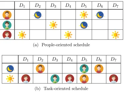
A medical schedule is the association of medical tasks with physicians and it can be represented as a table. There are two ways to look at a schedule: the people-oriented schedule that show the schedule of a group of employees, and the task-oriented that show the assignment of a set of tasks. Both types of schedule can be illustrated in a table where the columns represent the periods of the schedule, such as weeks, days or work shifts. In the people-oriented schedule, the employees are placed on the rows of the table and the assigned tasks are placed in the cells. In the task-oriented schedule, the tasks are on the rows and the employees are in the cells.

The tasks of a medical schedule can be general such as night and day shifts. They can also be more refined such as on-call tasks, clinic hours with patients, planned surgeries, emergency room tasks, research, etc. The length of a task can be an hour to a few days. We refer to the time over which the schedule spans as the horizon of the schedule. Figure 1.1 illustrates both representations for the same schedule with day and night shifts with a horizon of seven days.1

Note that the schedule in Figure 1.1 is incomplete, meaning that some of the tasks are not yet assigned. This is common for schedules in PetalMD’s database as explained in Section 1.2.

1

Sun and moon icons were created by katemangostar (https://www.freepik.com/free-photos-vectors/ winter). People avatars used in the current thesis were created by Freepik (https://www.freepik.com/ free-photos-vectors/people).

D1 D2 D3 D4 D5 D6 D7

(a) People-oriented schedule

D1 D2 D3 D4 D5 D6 D7

(b) Task-oriented schedule

Figure 1.1: Two representations of the same schedule with 3 employees and 2 tasks (day and night shifts)

However one chooses to represent a schedule, building a schedule requires assigning tasks to employees, or resources in general. Some tasks may require more than one employee to be considered fully assigned and some tasks may be defined for a subset of days only. The person in charge of making the schedule is called a planner.

1.2

Industrial context

There are conditions to meet to obtain a valid schedule which are constraints that cannot be violated. From observations made on PetalMD’s database, we can regroup the constraints of our context into five constraint families. Each instance in PetalMD’s database is made of a subset of the following constraints with different parameters. The general mathematical expressions encoding the constraints below are given in Section 4.4.

1. Unavailabilities and skills: determine if an employee is unavailable or unskilled for a given task. In Figure 1.1 for example, the third employee ( ) might not be skilled to execute the tasks occurring during the night shifts. Consequently, he is never assigned at night.

2. Exclusive constraints: forbids a group of employees to be assigned simultaneously (on the same time period) to a task from set T1 and a task from set T2. In Figure 1.1, each

employee is assigned to a single task each day.

3. Limiting constraints: determine the limit on the number of tasks a group of employees can be assigned within a subset of tasks. In Figure 1.1, each employee has no more than

1-night shift over 4 consecutive days. Moreover, the second employee ( ) has no more than 1-night shift over 7 consecutive days.

4. Variety limiting constraints: determine the limit on the number of different subsets of tasks a group of employees can be assigned to. For example, the following constraint is satisfied in Figure 1.1: “The last employee ( ) must be assigned to at most one task every 7 days.” This means that the employee is either assigned night shifts or day shifts but never both.

5. Employee limiting constraints: determine the limit on the number of employees from a team E that can be assigned to a subset of tasks T . The following constraint is satisfied in Figure 1.1: “The night shift ( ) should be assigned to at most 2 different employees.” Indeed, only the first two employees ( and ) are assigned to night shifts.

As it happens often in medical scheduling, the constraints are sometimes contradictory, meaning it is impossible to satisfy all constraints at once. There are two ways to obtain a solution in this context. Either we relax some of the constraints and allow some violations, or we create a partially filled schedule satisfying all constraints but leaving some tasks unassigned. PetalMD, our industrial partner, has observed that violations of constraints are not accepted by the employees of their clients. In our opinion, the reason for this rejection is that the scheduling tool used is not able to justify why one physician should work on a Saturday instead of another physician when both assignments would result in the violation of a constraint. The company has observed on the other hand that violations made by the planner are accepted more easily. PetalMD has chosen to create a partially filled schedule when building their business model and the planner needs to complete the schedule manually. Therefore, a valid schedule in our context is a schedule satisfying all constraints simultaneously. Moreover, we want to reduce as much as possible the number of tasks to assign manually. In addition to simplifying the planner’s task, most of the medical tasks are very important and need to be assigned. For example, shifts in an emergency room are vital. This is an other reason for maximizing the number of assigned tasks in the creation of a schedule.

In addition to the constraints that define the validity of a schedule, there are preferences (objectives) that determine the quality of a schedule. Violating preferences does not create an invalid schedule. For this reason, we do not consider them part of the constraints of the problem. However, we want to find a schedule satisfying the maximum number of preferences. The preferences are different from one client to another, or one employee to another. Some people might prefer not to work on Mondays. Others might prefer to work long days if they can avoid working on the week-ends, etc. In this thesis, we focus on preferences that concern the fairness of the schedule. A fair schedule would for example assign the same workload or the same task types to all employees.

Number of assigned tasks When constraints are contradictory, our first preference (objective) is to maximize the number of tasks that are assigned in the schedule.

Balance Planners want to produce well-balanced schedules. They want the assigned tasks to be spread over the horizon and spread over the employees. Moreover, employees must have a diversity of tasks assigned to them. Balancing workload in a schedule is a way to produce a fair schedule for all employees. There are multiple ways to define the balance of a schedule, Section 1.5 explains in more details what they are and how we study them in this thesis.

Workload targets Employees might have workload targets’ preferences. For example, one employee might want to have a total of 10-night shifts and 35-day shifts over the scheduling horizon. Usually, the targets are conflicting with one another and it is impossible to satisfy them all at once. Therefore, we want to create a schedule as close as possible to the targets. The workload targets are another way of determining what is a fair schedule, since they are often dictated by internal rules. For example, a senior employee might have a smaller target while a junior might have a larger target.

The preferences can be contradictory. For example, it is generally easier to balance a schedule with fewer assigned tasks since there is more room in the schedule to move assignments around. Thus, maximizing the balance and maximizing the number of assigned tasks are two conflicting objectives. When optimizing multiple objectives, one needs to make compromises. The management of multiple objectives in an optimization problem is called multi-objective optimization.

There are many different ways to deal with multi-objective optimization problems. One can use lexicographic order by defining a total order of preference on the objectives. To compare two solutions, we compare them according to the first objective. If both solutions have the same objective value for this first objective, we compare the solutions according to the second objective, and so on.

There is also the optimal Pareto frontier technique, which separates solutions into two categories : the dominated solutions and the non-dominated solutions. A solution B is dominated by a solution A if it has a lower objective value for all objectives. The non-dominated solutions form the optimal Pareto frontier, where they each dominate another solution according to at least one objective. Therefore, from a mathematical point of view, all solutions of the Pareto frontier are equivalent. The planner can then choose one solution form the Pareto frontier and at the same time choose which compromises to make.

We do not study multi-objective techniques in this thesis, but the proposed optimization models of Chapter 4 are built so the multi-objective technique can easily be changed.

1.3

The importance of automated scheduling

In this thesis, we focus on improving the quality of physicians’ schedules by using automated scheduling. There are many advantages to automated scheduling.

1. It is faster. While a human tests a single schedule, a computer can test several thousands. 2. The obtained schedules are of better quality. If a computer can test thousands of

schedules, it can find better solutions than a human can imagine.

3. It is cheaper than manual scheduling. 10 hours of machine time is less expensive than one hour of the physician’s time.

4. It is easier. When building a schedule using a pre-configured automated scheduling system, the planner requires close to no scheduling expertise.

There are of course some drawbacks to automated scheduling.

1. It requires a high-level mathematical knowledge to configure the scheduling system. 2. It requires a certain degree of vulgarization so the planner without mathematical

knowledge can use the system.

3. It requires a solver that can efficiently solve the given models.

4. The quality and validity of a solution are often not obvious to the planner.

While developing and maintaining an automated scheduling system is costly, it is preferable when a large number of schedules are created. In the case of PetalMD for example, thousands of clients on the platform create a few schedules a year. Overall, manually creating the schedules costs a lot more than the system.

PetalMD’s scheduling tool is not accessible to all of the company’s clients. Each new client who wants to use the scheduling tool must contact the customer service and talk with an expert that will create a mathematical model corresponding to the client’s problem. In other words, the expert looks at the previous schedules that the client manually created and must deduce the real constraints of the problem. The clients rarely have the necessary training to verbalize their constraints. We can, however, suppose that any client is able to say if a given schedule is valid or not.

The process of adding constraints to the scheduling tool is complicated and require a great deal of time for both the client and the company. To reduce the time induced by the addition of new clients to the scheduling tool and to enable the clients to create their own mathematical

models, we need to supply them an improved scheduling tool that can guide them through the process.

We study two different aspects of automated scheduling: mathematical modeling to automatically create schedules and constraint acquisition which automatically builds the mathematical model from given schedules. Mathematical modeling is the process of writing the problem (tasks, employees, constraints, and goals) with mathematical expressions. Then, a software called solver usually solves automatically when possible the given mathematical model and returns one or more solutions. We propose mathematical models in Chapters 3 and 4 to optimize the balance in schedules. Constraint acquisition is the process of learning from a set of positive solutions, in our case valid schedules, the constraints that created the examples. The acquired information can then be used to automatically create a mathematical model that can in turn automatically produce new solutions (valid schedules). We present techniques to learn the mathematical model from given schedules in Chapter 5. We focus on learning parameters for global constraints (see Section 2.1.5 for the definition of a few global constraints), this ensures a more efficient modeling process. However, we do not study how to optimize a learned model.

1.4

Related problems

We have introduced a global scheduling problem, but there are several other problems in medical scheduling. Hall [52] presents in his book Handbook of Healthcare System Scheduling some of the more important categories of problems.

An important and widely studied problem in medical scheduling is the nurse scheduling problem (NSP). It consists of assigning shifts to nurses that have different skills while satisfying preferences as much as possible. Multiple papers study this problem, such as Ogulata et al. [81] who propose an integer programming model. Tsai et al. [107] address this problem with a two-stage mathematical model using a genetic algorithm. The first stage finds schedules satisfying the constraints and optimizing the preferences, and the second stage assigns the schedules to the nurses while re-optimizing. Brucker et al. [34] propose another two-stage model using a greedy local search to build the final schedule. Qu and He [95] propose a two-stage approach combining constraint programming and variable neighborhood search. The constraint programming model finds high-quality shift sequences and the variable neighborhood search is used to improve the obtained solution. Burke et al. [35] address a multi-objective version of the NSP also using a hybrid model, this time combining integer programming and variable neighborhood search. In both cases, the mathematical model is used to find a solution satisfying the constraints of the problem and the variable neighborhood search is used to improve the solution so it satisfies the preferences as much as possible. The operating room scheduling problem has for goal to assign operating room times to surgeons.

Some instances consider elective surgeries, which can be planned in advance, others consider emergency surgeries, which occur randomly and must be performed quickly. The solution must sometime consider room availability and post-surgical resource constraints. Among the most recent papers, Fei et al. [44] propose a branch-and-price method that combines a branch-and-bound algorithm with a column generation technique. Lamiri et al. [59] address the problem with a Monte Carlo optimization method that uses both Monte Carlo simulation and mixed integer programming. Beliën and Demeulemeester [17] address the combined nurse and operating room scheduling problem using integer programming with column generation. The patient appointments in ambulatory care problem assigns time periods to patients in a walk-in context while complying with resource availability and preferences. The major difficulties of this problem lie with the no-shows, the random arrivals, and the fluctuating degrees of urgency of patients’ needs. Gupta and Wang [49] use a Markov decision process to model the appointment booking problem for a primary-care clinic, which they combine with heuristics.

The bed assignment and management problem consists of assigning beds to patients while minimizing the number of unoccupied beds and minimizing the number of waiting patients. Therefore, the goal is to synchronize discharges with admissions as much as possible. Moreover, bed management must take into account other hospital requirements and it should not delay surgeries and other provided care. Bekker and Koeleman [9] propose a quadratic programming model to compute the ideal number of per day admissions. This data is used to create guidelines and practical scenarios that hospital managers can use. Li et al. [64] use model based on queuing theory and goal programming to optimize bed allocation in a hospital in a two-stage approach. The queuing theory is first used to determine typical features of the hospital. From those results, they build a multi-objective model based on goal programming. The On-call Scheduling Problem consists of assigning night shifts to physicians while satisfying skill and staffing requirements and satisfying the preferences as much as possible. Wang et al. [111] solve this problem using genetic algorithms, while Sherali et al. [105] use mixed integer programming (see Chapter 2.2) coupled with heuristics.

The workload distribution among physicians or nurses problem aims to assign equal workloads to physicians or nurses. Beaulieu et al. [7] impose lower and upper limits on the number of shifts a physician can do in the form of linear constraints. All the linear constraints combined ensure that tasks are distributed over the physicians. Lanzarone et al. [60] minimize the deviation from the capacity of a nurse, the maximum number of patients a nurse should be assigned to by his/her contract, with the help of a quadratic cost function. One version of this problem, the balancing nursing workload problem, can be found in CSPLib2_{. Mullinax and Lawley [79]}

assign patients to nurses in a neonatal intensive care unit divided into multiple zones. To

2

ensure a fair distribution, they minimize the difference between the maximum and minimum workloads for each zone in an integer linear program. Schaus et al. [103] tackle this problem using a constraint programming model while Ku et al. [57] solve it by incorporating constraints taken from Schaus et al.’s model inside a mixed integer quadratic programming model. Often in the literature, the medical scheduling problem is divided into subproblems, for each type of tasks. In this thesis, we address the physician scheduling problem as a whole and we do not separate the different tasks.

1.5

Balancing a schedule

The quality of a medical schedule can make a difference in the quality of medical care provided [66]. For example, physicians are prone to make mistakes when they are overworked. However, while the quality of a physician’s schedule is important, it is even more important that certain tasks are covered. In other words, it is more important that certain tasks, such as emergency room tasks, are assigned to the proper number of physicians.

One important quality feature of a schedule is the balance. There are several ways to define the balance of a schedule. We present three of those definitions here. The first two are addressed in Chapter 3 with balancing constraints. The last balance definitions are addressed in Chapter 4 with linear optimization models.

1.5.1 Uniform workloads

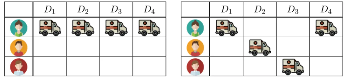
One type of balance is the uniform distribution of tasks among all the employees. In other words, in this context we want all employees to have the same amount of work. Therefore, the problem consists of determining workload targets for each employee and creating schedules for which the workloads are as close as possible to the predetermined targets. This can be applied to all tasks at the same time or to a certain type (clinic, on-call, emergency room, surgeries, etc.). For example, suppose we want to distribute emergency room tasks between three physicians on a horizon of four days. Figure 1.2 illustrates two distributions scenarios : Scenario A where all emergency room tasks are assigned to the first physician and Scenario B where only the first physician is assigned more than one task. Since we are distributing four tasks among three physicians, at least one physician must be assigned two tasks. Therefore, Scenario B represents an optimal distribution of the workloads.

1.5.2 Uniform variety

Another type of balance is the uniform distribution of each task to an employee. It is similar to uniform workloads, but we want to assign the same amount of each task to an employee. For example, suppose we have three tasks, emergency room ( ), surgery ( ), and research ( ),

D1 D2 D3 D4

(a) Scenario A: Workloads poorly distributed

D1 D2 D3 D4

(b) Scenario B: Workloads well distributed

Figure 1.2: Two different scenarios for the distribution of workloads among three physicians over a scheduling horizon of four days.

to assign to a physician over an horizon of four days. 3 _{If we assign the maximum number of}

tasks each day, then we have a similar situation to the balance of uniform workloads. Figure 1.3 illustrates two scenarios for the balance of task types : Scenario A where only the first task is assigned and Scenario B where each task is assigned once except one ( ) which is assigned twice.

D1 D2 D3 D4

(a) Scenario A: Poorly distributed

D1 D2 D3 D4

(b) Scenario B: Well distributed

Figure 1.3: Two different scenarios for the distribution of task types for a physician over a scheduling horizon of four days.

1.5.3 Uniform distribution

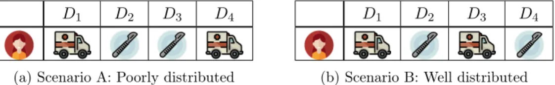
Another way to define balance is over time. Here, we want to evenly distribute an employee’s tasks over the scheduling horizon, meaning that we want the distance between each couple of consecutive tasks to be the same. Consider a four-day scheduling example with one employee and two types of tasks, emergency room ( ) and surgery ( ). We want a schedule where the emergency room tasks are as evenly distributed over the scheduling horizon as possible. After removing symmetries, there are two different scenarios as illustrated in Figure 1.4. Even though Scenario A seems to be well distributed, Scenario B is a better long-term choice because we might need to create multiple successive schedules. This becomes obvious if we repeat each scenario, as in Figure 1.5. Scenario A creates clusters of emergency room tasks at the junction of the two schedules while no clusters are created by Scenario B.

Since we want to spread the emergency room tasks as much as possible in the scheduling period, we want to maximize the number of days (or other time periods) between two emergency tasks. Let us consider the scenarios of Figure 1.4 without the surgery tasks. We refer to the days between two considered tasks as a spacing. Maximizing the number of days between emergency

3

D1 D2 D3 D4

(a) Scenario A: Poorly distributed

D1 D2 D3 D4

(b) Scenario B: Well distributed

Figure 1.4: Two different scenarios for the same physician with two tasks, emergency room and surgery.

D1 D2 D3 D4 D5 D6 D7 D8

(a) Scenario A: Poorly distributed

D1 D2 D3 D4 D5 D6 D7 D8

(b) Scenario B: Well distributed

Figure 1.5: Each pattern is repeated once showing the effect of repeating a poorly distributed pattern.

tasks is equivalent to maximizing the length of each spacing. The spacings of both scenarios are illustrated in Figure 1.6 using arcs.

(a) Scenario A: Poorly distributed (b) Scenario B: Well distributed

Figure 1.6: Two scenarios with different spacings. The first schedule has one spacing of length 2 and one of length 0. The second schedule has two spacings of length 1.

For a given schedule, we know the number of assigned emergency room tasks and we can compute the ideal length of the spacings. For example, with a scheduling horizon of 4 days and 2 assigned emergency tasks, the ideal situation is illustrated with Scenario B where emergency room tasks alternate with other tasks or days off. Thus, the ideal length is one day.

To identify if the tasks of a schedule are well distributed or not, we can use a metric computing the difference between the actual spacings’ length in the schedule and the ideal length. There are several possible metrics. For instance, one can compute the absolute distance between the minimum length and the ideal length. Or, one can compute the sum over the squared distances between each spacing length and the ideal length. We propose a metric to compute the quality of a schedule according to its distribution in Chapter 4 and we also propose two models to optimize the distribution of events during the creation of a schedule.

1.6

Other balancing problems

Balancing solutions have other applications than medical scheduling. For instance, in the balanced academic curriculum problem4 _{(BACP) proposed by Castro and Manzano [37], the}

goal is to assign periods of time to courses while distributing the workload over all the periods in order to create a balanced curriculum. There are multiple papers that study the distribution of events or the balancing of solutions in one form or another. Here is a short list of important problems on balancing schedules and workloads.

The exam timetabling problem consists of assigning time slots and rooms to exams. One of the earliest paper published on this problem is proposed by Broder [33]. One of the goals is generally to space out the exams as much as possible in a non-cyclic scheduling period. Al-Yakoob et al. [2] propose models with hard and soft constraints limiting the clusters of exams, thus maximizing the distribution of exams across the scheduling horizon. MirHassani [75] defines three categories of undesirable situations and classifies them in order of student’s depreciation. The objective is to minimize the number of undesirable situations of each category with weighted sums encoding their priority. McCollum et al. [74] impose a limit of one exam per x consecutive days. Each additional exam counts for one in a penalty function. In addition to this objective, their model includes the minimization of the number of two consecutive exams and the number of days with two exams.

Another related problem is the balanced academic curriculum problem 5 _{(BACP). The goal of}

BACP is to assign courses to time periods, following a set of administrative rules, in a way that ensures the academic load is as similar as possible between periods. Castro and Manzano [37] compare a constraint programming approach to an integer programming approach. They show that the combination of a constraint programming model with clever heuristics is able to solve more instances than an integer programming model. Hnich et al. [53] propose a hybrid model composed of constraint programming and integer programming to solve the balanced academic curriculum problem. Their approach is separated into two phases in order to take advantage of both resolution techniques strengths. Lambert et al. [58] also tackle the problem with a hybrid approach, this time using a combination of constraint programming and genetic algorithms. Monette et al. [76] build on the constraint programming model proposed by Hnich et al. [53]. Among their contributions, they present a heuristic for value ordering and other balance criteria. Chiarandini et al. [39] study a generalized version of the balanced academic curriculum problem. They propose new objective functions which are better adapted to this new problem and they test their models on real-life instances from the University of Udine, Italy.

The distribution of events in a schedule makes sure that the spaces between those events are as

4

prob030 in CSPLIB (www.csplib.org)

5

equal as possible. The problem of balancing workloads among employees consists in assigning the same number of events to every employee. Both problems aim at equalizing quantities and are therefore related. Hence, models for the workload balancing problem can be used to distribute events in a schedule if combined with a model to compute the distance between events.

Workload balancing among employees is also studied for the traveling workers problem or the crew drivers problem. Beaumont [8] studies the problem of finding cyclic patterns for work days and days off for traveling workers. The rostering horizon is split into non-overlapping 30-day sub-horizons. The objective is to have the same amount of worked days for each of the 30-day sub-horizons. To achieve this goal, they compute the ideal number of worked days (target) per 30 days and minimize the absolute deviation from the 30-day target for each sub-horizon. Bianco et al. [30] minimize the maximum workload in the rostering problem of crew drivers to distribute the workload. This technique has for drawback that all workloads smaller than the maximum workload are ignored while they could still be distributed.

Ásgeirsson and Sigurðardóttir [4] study two different distribution situations in the self-scheduling problem: the spreading of the understaffed and overstaffed shifts in order to avoid the concentration of over/under-staffing on a single shift and the spreading of unfulfilled requests among the workers. Both of these situations are tackled by implementing piecewise linear penalty functions increasing the cost of deviations.

1.7

Other constraint acquisition problems

We presented multiple papers addressing the balancing of solutions and the distribution of events in Sections 1.5 and 1.6. Now we present important papers studying the second subject of this thesis: constraint acquisition. There exist multiple approaches to constraint acquisition, the process of learning the constraints of a model from its solutions.

Bessiere et al. in [24, 25, 29, 40] propose an algorithm named ConAcq learning constraint networks from positive and negative solutions using version space learning. Version space learning defines the search space for the constraint network as a set of constraint network candidates (hypothesis). Each hypothesis not satisfied by all positive examples is removed. ConAcq encodes each example as a set of clauses where the atoms are taken from the constraint vocabulary of the library of constraints. A solution to the corresponding satisfiability problem is, therefore, an admissible constraint network.

O’Connel et al. [80] present an interactive version space algorithm, which creates a first version space from examples given by the user. From one of the hypotheses, the system builds a qualifying example. The user accepts or rejects it, and the version space is updated accordingly. The algorithm terminates when the version space contains a single hypothesis.

Bessiere et al. [23] offer an active learning system named QuAcq. QuAcq adds one constraint at a time in the network by presenting partial queries, which are classified by the user as positive or negative. QuAcq chooses queries that satisfy the constraints in the current network and violate at least one constraint in the library until no such queries exist. Arcangioli and Lazaar [3] propose an improvement on QuAcq called MultiAcq that detects multiple violated constraints from a negative example instead of the single violated constraint returned by QuAcq.

Beldiceanu and Simonis [15, 12] introduce the Constraint Seeker, that includes a web-based interface that allows a user to search for a global constraint in the Global Constraint Catalog [13] using positive and negative examples. The user is considered to have a good comprehension of the constraint in natural language but he/she does not know the corresponding constraint in the Global Constraint Catalog. Moreover, the variables on which the constraint is applied are unknown. Beldiceanu and Simonis [16, 11] propose a constraint acquisition tool they refer to as Model Seeker. This tool builds a satisfaction model from positive examples using constraints from the global constraint catalog. The Model Seeker creates a list of candidates, all global constraints satisfying the examples, by generating sequences and matching them against the global constraints using the Constraint Seeker. The candidates are ordered according to their pertinence, which is computed using multiple criteria, such as solution density and constraint popularity. A dominance check is performed to remove redundant constraints. One criterion is the number of assignments that satisfy the constraint. If this number is small, that indicates that the solutions come from a small subset of possible assignments. This is more likely to occur if the constraint was imposed.

Bessiere et al. [21, 22], Bartak et al. [5], and Charnley et al. [38] study the acquisition of implied constraints from a CSP in order to improve the resolution time. Bessiere et al. [20] use the examples to remove redundant constraints from the model during the constraint acquisition phase.

Kiziltan et al. [55], Little et al. [65], and Lopez and Lallouet [68] study the translation of a problem description written in natural language into a formal model.

Machine learning techniques can also be used to learn part of a model. Bonfietti et al. [31], Bartolini et al. [6], and Lombardi et al. [67] train neural networks or decision trees to recognize a solution to a problem and then embed the trained neural network or the trained decision trees into a global constraint. This constraint restrains the solver to return a solution that would be classified as a positive example by the neural network or the decision trees.

Campigotto et al. [36] and Kolb [56] study the acquisition of the utility function of the optimization model.

parameters are specific to a problem and determine the context in which the constraint is used. Suraweera et al. [106] propose a system that learns parameters for template constraints previously defined from historical schedules. Their system can learn parameters for three types of constraints :

1. An implication of assignments which imposes that a given variable is equal to a given value when a set of variables take specific values,

2. A conjunction of simple inequalities on real variables which imposes lower and upper bounds on given variables,

3. Nested implication constraints defining a decision tree.

Some of the challenges addressed by Suraweera et al. include the detection of variables’ domains and the scope of the constraint.

Chapter 2

Combinatorial Optimization

The goal of the current thesis is to improve the quality of medical schedules. We use mathematical modeling to encode the objectives and rules of a schedule in Chapter 4. We give the model to a solver which solves it and returns a feasible solution, a valid schedule. We also use mathematical modeling to compute probabilities in Chapter 5. The scheduling rules and objectives of Chapter 4 and the probability computation of Chapter 5 are both combinatorial problems, which we describe in the current chapter.

There are two large families of optimization problems: the ones with continuous (real) variables and the ones with integer variables. The latter is called Combinatorial Optimization and consists of finding an optimal solution among a finite or countable infinite set. Therefore, the optimal solution is a combination of possible discrete values.

In this chapter, we introduce the basic concept of optimization problems and different types of problems such as constraint satisfaction problems and mixed integer programs. We also present resolution techniques for these problems: search trees, filtering, the Simplex method, etc.

Section 2.1 presents a resolution technique for combinatorial problems. Section 2.1.1 explains the difference between the mathematical models of a satisfaction problem and an optimization problem. Sections 2.1.2, 2.1.3, and 2.1.4 describe how the solutions of a satisfaction or optimization problem can be found by ingeniously exploring assignments. Different constraints and their configuration are presented in Section 2.1.5. The literature on how to count the solutions of a given constraint is detailed in Section 2.1.6. Section 2.2 presents problems with both integer and real variables and describes how matrix properties can be used to solve them efficiently. A specific problem, called flow network, is introduced in Section 2.3 as a mathematical model because it has the matrix property discussed in Section 2.2. Finally, another mathematical model, called Markov chains, is described in Section 2.4 as an efficient mathematical tool to compute probabilities, which we use later in Chapter 5.

2.1

Constraint Programming

Constraint programming (CP) is a technique to solve combinatorial problems of all sorts: scheduling, vehicle routing, networks, and more. The general idea of constraint programming is that one encodes a problem using mathematical formulation and a solver uses this model to find a solution. The basic problem in constraint programming is called constraint satisfaction problem (CSP), see Section 2.1.1 for a definition. The usual form of a CSP was introduced by Montarini [77] and Mackworth [70]. Multiple generalizations of the usual CSP have been proposed afterward, such as the constraint optimization problem (COP) [19, 43].

As explained in the Handbook of Constraint Programming [19], constraint programming is part “mathematical programming”, where one needs to encode a problem with a mathematical model and use a solver to find a solution, and part “computer programming”, where one needs to program a search strategy to find the solution. Both the quality of the model and the quality of the search strategy are important in constraint programming to have an efficient solving method.

2.1.1 Satisfaction and optimization problems

Constraint programming solves constraint satisfaction problems, which are defined by variables, domains, and constraints. While an assignment [X1, . . . , Xn]determines the values

assigned to each variable, the domain of a variable X, noted dom(X), is a set of values that can be assigned to X. A constraint C([X1, . . . , Xn]), where n is called arity of C, is a relation

over the set of variables [X1, . . . , Xn], called the scope of C, restricting the values that they

can take simultaneously.

A constraint satisfaction problem (CSP) is composed of a set of variables [X1, . . . , Xn] and

a set of constraints C. The goal is to find an assignment ~X satisfying all constraints in C simultaneously. Such an assignment is called feasible point, feasible assignment, or feasible solution and F the set of all assignments satisfying C is called feasible set.

A well-known constraint satisfaction problem is the Boolean satisfiability problem or simply the SAT problem. A SAT problem is defined by ~X = [X1, . . . , Xn] ∈ {true, false}n, a set

of Boolean variables, and Φ( ~X), a Boolean formula. A valid assignment ~X evaluates Φ( ~X) to true. A literal Li is a variable in {X1, . . . , Xn, ¬X1, . . . , ¬Xn}. The Boolean formula

of a SAT problem is generally formulated as a list (conjunction) of disjunctive expressions C = {c1, . . . , cm} called clauses. In other words, each clause is a disjunction of literals,

cj = Lj1∨ · · · ∨ Ljdj, and a valid assignment ~X ensures that all clauses evaluates to true

simultaneously.

3-SAT is a specific case of SAT where each clause has exactly three (3) literals. Both SAT and 3-SAT are NP-hard problems. We use 3-SAT in Chapters 3 and 5 to demonstrate that

two other problems are also NP-hard. For more information about SAT or 3-SAT, the reader is referred to Chapter 34 of Cormen et al. [41].

Adding the optimization of an objective function f([X1, . . . , Xn]) to a constraint satisfaction

problem creates a constraint optimization problem (optimization problem or COP). The goal is to find a feasible assignment [X1, . . . , Xn]that optimizes the value of f([X1, . . . , Xn]). For

complement information, the reader is referred to the Handbook of Constraint Programming [19]. The objective function of a COP can be any function: exponential, quadratic, linear, transcendental, etc. In this thesis, we often use linear functions since they correspond directly to many real problems and they represent the intuitive choice in most cases. Moreover, solving a problem with a linear objective is easier since the function is convex.

In an optimization problem, an assignment ~X = [X1, . . . , Xn]is locally optimal if it is the best

solution among all other solutions close to ~X. The distance between solutions is computed using metrics (such as the Euclidean distance) or transformation operators. ~X is said to be globally optimal if there are no better solutions than ~X. When solving an optimization problem, one wants to find a globally optimal solution ~X. The convexity of the objective function and the feasible set has a huge impact on the complexity of solving the optimization problem.

A set of points S ⊆ Rn _{is convex if for every pair x, y ∈ S we have z ∈ S for every}

z = λx + (1 − λ)y, 0 ≤ λ ≤ 1.

A function f : S → R, where S is a convex set, is said to be convex in S if for every pair x, y ∈ S

f (λx + (1 − λ)y) ≤ λf (x) + (1 − λ)f (y), 0 ≤ λ ≤ 1.

Convex optimization problems are optimization problems for which both the objective function and the feasible set are convex. The locally optimal solutions of these problems are also globally optimal. Solving a non-convex problem is hard since the solver might not be able to distinguish a locally optimal solution from a globally optimal one. Therefore, working with convex problems is a better choice when it is possible. More information on convex optimization problems can be found in [84].

2.1.2 Search tree

To find a solution to a satisfaction problem or an optimal solution for an optimization problem, we can use a search tree. The general idea is to explore all possible assignments by temporarily adding constraints to the problem, often of the form of an equality beween a variable and a constant. This equality fixes the variable to its value. While other forms of constraints can also be used, this thesis only consider such equality constraints. We create the search tree as

follows. The nodes represent the partial assignments for which some variables have been fixed and some are still free. The root of the tree is the partial assignment where all variables are still free. Usually, we fix one variable per level in the tree and we travel the tree from top to bottom and from left to right. This means that we visit the children of a node before its neighbor. This technique is called depth-first search.

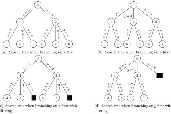
Example 1. Suppose that we want to find all solutions to the constraint X + Y ≤ 8 with dom(X) = {3, 4} and dom(Y ) = {1, 4, 8}. Figure 2.1 illustrates two different branching trees for this problem.

0 1 3 y= 1 4 y = 4 5 y = 8 x= 3 2 6 y= 1 7 y = 4 8 y = 8 x = 4

(a) Search tree when branching on x first

0 1 3 x= 3 4 x = 4 y= 1 2 6 x= 3 7 x = 4 y = 4 2 6 x= 3 7 x = 4 y = 8

(b) Search tree when branching on y first

0 1 3 y= 1 4 y = 4 5 y = 8 x= 3 2 6 y= 1 7 y = 4 8 y = 8 x = 4

(c) Search tree when branching on x first with filtering 0 1 3 x= 3 4 x = 4 y= 1 2 6 x= 3 7 x = 4 y = 4 X y₌ 8

(d) Search tree when branching on y first with filtering

Figure 2.1: Different versions of a search tree depending on branching order and if filtering is applied.

The search tree grows exponentially with the number of variables and the number of values in the domains. For example, suppose we have n variables and if all domains contain m values. In the worst case, the total number of leaves is mn _{and the total number of nodes in the tree}

is _n X i=0 mi= m n+1_{− 1} m − 1 ,

which is also in Θ(mn_{). Some of these nodes do not lead to solutions and removing them could}

greatly reduce the resolution time. This pruning can be achieved by filtering values which do not participate in valid assignments.

2.1.3 Filtering and constraint propagation

To cut branches that do not lead to solutions in the search tree, we can test and remove the values that are inconsistent with the constraints of the problem at each node of the tree. To determine if a value v ∈ dom(Xi)is inconsistent for a given constraint, we test whether there

is an assignment with the current domains that assigns v to Xiwhile satisfying the constraint.

An assignment ~α satisfying a constraint C and such that αi = vand αi ∈ dom(Xi) for all i is

a domain support for the value v ∈ dom(Xi) and for the constraint C.

A constraint C([X1, . . . , Xn]) is said to be domain consistent if and only if for every variable

Xi there exists a domain support for each value v ∈ dom(Xi) and constraint C. A set of

constraints C is said to be locally consistent if all constraints in the set are domain consistent. A filtering algorithm for a constraint C( ~X) is a specific algorithm for the constraint that removes values from the domains of ~X until C has the desired consistency, in our case domain consistency.

We can apply the filtering algorithms of the constraints on each node of the search tree to remove all values that do not have a support and obtain local consistency. This cuts out branches that do not lead to solutions and reduces the time required to find the solutions. Constraint propagation is a technique that calls the filtering algorithms of a set of constraints in order to obtain local consistency. There are various constraint propagation algorithms. The most popular propagation algorithm, called AC-3, was proposed by Mackworth [70]. It achieves local consistency on a constraint set where all constraints have an arity of 2. Mackworth [71] proposed an extended version of the algorithm that achieves local consistency for constraint sets with arbitrary arities. The idea is to keep a list of all potentially inconsistent constraints. Every time a filtering algorithm modifies the domain of the variable Xi, we add all

constraints that have Xi in their scope. The algorithm stops when the list is empty, meaning

we have obtained local consistency, or when a domain is empty, meaning the problem has no solution.

Example 2. Let dom(A) = dom(B) = {1, 2, . . . , 10}. Suppose we have the constraints A + 3B = 12 and AB ≥ 10. When we apply domain consistency to this set of constraints, we obtain the results in Table 2.1.

Filtered constraint dom(A) dom(B) {1, 2, . . . , 10} {1, 2, . . . , 10} A + 3B = 12 {3, 6, 9} {1, 2, 3}

AB ≥ 10 {6, 9} {2, 3}

A + 3B = 12 {6} {2}

2.1.4 Branch-and-bound

When using a search tree to explore the solutions of an optimization problem, we can use the objective function to prune the search space. The idea is to not only filter the infeasible assignments, but also the suboptimal assignments.

We consider a general minimization problem where all variables must take positive integer values. The branch-and-bound requires an algorithm that can compute a lower bound on the given problem, where some of the variables might be fixed. This algorithm is called at each node of the search tree. The search tree gives us an upper bound on the objective value when a first feasible solution is found since any optimal solution must have an objective value lower or equal to any feasible solution. Other techniques such as approximation algorithms can also find upper bounds, refer to Chapter 35 of Cormen et al. [41] for more information. We keep track of the incumbent solution, the best-observed solution. All nodes of the search tree for which the lower bound is greater than the upper bound of the incumbent solution can be discarded since they can only lead to worst feasible solutions.

Ideally, the branch-and-bound algorithm stops when the lower bound is equal to the upper bound because this means we have found a feasible solution with the minimal objective value. In other words, when all unexplored nodes have a worst lower bound than the objective value of the incumbent solution, the incumbent solution is optimal. In larger problems, proving the optimality of an incumbent solution might be time-consuming or even impossible. In that case, a gap can be defined representing the allowed difference between both bounds. Note that even if the gap is not equal to zero, the current best solution might be optimal but we have no proof of optimality. In general, one considers a feasible solution to be optimal if the gap is small enough.

The quality of the bound is very important since a tighter bound cuts more branches of the search tree. The lowest value possible for the upper bound is the value of the objective function at its global optima. So the lower the bound, the closer to solving the problem we are and the harder it is to compute the bound. Therefore, there is a compromise to be made between the tightness of the bound and the complexity of the computation.

To this branch-and-bound technique, we can add strategies to improve the resolution time by reducing the number of expanded nodes. One of the well-known search strategies is called best-first search. The main idea is that we explore the node with the lowest lower bound first, since it has the highest potential in leading to the minimal objective value. Let N1 and N2

be two nodes of a branch-and-bound tree for a minimization problem and let Li be the lower

bound of node Ni. By definition of the lower bound, we have that all children Nj of a node

Ni are such that Lj ≥ Li. Therefore, if we have L1 < L2, then the best-first search technique

2.1.5 Global constraints

An elementary constraint is a constraint whose arity is constant. A global constraint is a constraint whose arity is a parameter. Let C([X1, . . . , Xn], [a1, . . . , am])be a global constraint

where [X1, . . . , Xn]are integer variables denoted in upper case and [a1, . . . , am]are parameters

denoted in lower case. For example, Sum([X1, . . . , Xn], a) is the global constraint and an

instantiation is X1 + X2 = 4 with parameters a = 4 and n = 2. In general, we use global

constraints to encode a complex relation between variables that requires multiple elementary constraints.

It is often possible to rewrite a global constraint using only simple constraints. A decomposition for a global constraint C( ~X, ~a) is a set C of simpler constraints such that an assignment ~α is a solution of C if and only if it is a solution of C( ~X, ~a). It is usually better to use the global constraint since it comes with a set of specialized filtering algorithms that reduce the search space by removing impossible assignments early on while using a decomposition might lead to a filtering loss. For instance, AllDifferent(X, Y, Z) on the domains dom(X) = dom(Y ) = dom(Z) = {1, 2} detect the lack of solution while the decomposition X 6= Y, Y 6= Z, X 6= Z is locally consistent. Moreover, some decompositions introduce new variables that are not fixed when the variables of the initial problem are fixed, which can also lead to filtering loss. However, since the filtering algorithms of certain global constraints are computationally demanding, we sometimes prefer to use decomposition even when they are less efficient with the filtering. Therefore, there is a compromise to be made between the required filtering time and the desired filtering level.

The most interesting global constraints are those for which there exists a filtering algorithm running in polynomial time. In general, these algorithms are based on well-known problems such as network flows, shortest paths, dynamic programming, etc.

Usually, there exist multiple valid decompositions for a single global constraint. A decomposition A is said to be stronger than a second decomposition B if the constraint propagation on A removes a superset of values than the constraint propagation on B.

In the rest of this thesis, we will need the following global constraints. Multiple global constraints are applied to a subset of values that we encode with a vector of parameters ~

z. We have that zv = 1 if the value v is in the set and zv = 0 otherwise. In other words,

the vector ~z is the bit set encoding of a set. For that reason, by abuse of notation, we will consider ~z sometimes as a binary vector, sometimes as a set of values.

AllDifferent([X1, . . . , Xn]) [100] ensures that the variables [X1, . . . , Xn] take distinct

values. This constraint can model a set of tasks that must be executed by different employees, where Xi is the employee assigned to the task i and dom(Xi) is the set of employees that can