HAL Id: hal-02315471
https://hal.archives-ouvertes.fr/hal-02315471
Submitted on 14 Oct 2019
HAL is a multi-disciplinary open access
archive for the deposit and dissemination of
sci-entific research documents, whether they are
pub-lished or not. The documents may come from
teaching and research institutions in France or
abroad, or from public or private research centers.
L’archive ouverte pluridisciplinaire HAL, est
destinée au dépôt et à la diffusion de documents
scientifiques de niveau recherche, publiés ou non,
émanant des établissements d’enseignement et de
recherche français ou étrangers, des laboratoires
publics ou privés.
To cite this version:
T-H. Hubert Chan, Arnaud Guerqin, Mauro Sozio. Fully Dynamic k -Center Clustering. 2018
World Wide Web Conference, Apr 2018, Lyon, France. pp.579-587, �10.1145/3178876.3186124�.
�hal-02315471�
Fully Dynamic k-Center Clustering
∗
T-H. Hubert Chan
†University of Hong Kong Hong Kong [email protected]
Arnaud Guerquin
LTCI, Télécom ParisTech University Paris, France
Mauro Sozio
‡LTCI, Télécom ParisTech University Paris, France
ABSTRACT
Static and dynamic clustering algorithms are a fundamental tool in any machine learning library. Most of the e�orts in developing dynamic machine learning and data mining algorithms have been focusing on the sliding window model (where at any given point in time only the most recent data items are retained) or more simplistic models. However, in many real-world applications one might need to deal with arbitrary deletions and insertions. For example, one might need to remove data items that are not necessarily the oldest ones, because they have been� agged as containing inappropriate content or due to privacy concerns. Clustering trajectory data might also require to deal with more general update operations.
We develop a (2 + )-approximation algorithm for the k-center clustering problem with “small” amortized cost under the fully dynamic adversarial model. In such a model, points can be added or removed arbitrarily, provided that the adversary does not have access to the random choices of our algorithm. The amortized cost of our algorithm is poly-logarithmic when the ratio between the maximum and minimum distance between any two points in input is bounded by a polynomial, while k and are constant. Our theo-retical results are complemented with an extensive experimental evaluation on dynamic data from Twitter, Flickr, as well as trajec-tory data, demonstrating the e�ectiveness of our approach.
ACM Reference Format:
T-H. Hubert Chan, Arnaud Guerquin, and Mauro Sozio. 2018. Fully Dynamic k-Center Clustering. In WWW 2018: The 2018 Web Conference, April 23–27, 2018, Lyon, France. ACM, New York, NY, USA, 9 pages. https://doi.org/10. 1145/3178876.3186124
1 INTRODUCTION
With over 6000 tweets per second being posted on Twitter, Google processing over 40000 queries every second, and more than 400 hours worth of youtube videos uploaded every minute, there is an urgent need to develop dynamic machine learning and data mining
∗This research was partially supported by a grant from the PROCORE France-Hong
Kong Joint Research Scheme sponsored by the Research Grants Council of Hong Kong and the Consulate General of France in Hong Kong under the project F-HKU702/16.
†This research was partially supported by the Hong Kong RGC under the grants
17217716.
‡This research was partially supported by French National Agency (ANR) under
project FIELDS (ANR-15-CE23- 0006).
This paper is published under the Creative Commons Attribution 4.0 International (CC BY 4.0) license. Authors reserve their rights to disseminate the work on their personal and corporate Web sites with the appropriate attribution.
WWW 2018, April 23–27, 2018, Lyon, France
© 2018 IW3C2 (International World Wide Web Conference Committee), published under Creative Commons CC BY 4.0 License.
ACM ISBN 978-1-4503-5639-8/18/04. https://doi.org/10.1145/3178876.3186124
algorithms. Most of the e�orts in this direction have been focusing on the sliding window model of computation [6, 7], where at any given point in time only the most recent data items are retained, or more simplistic models.
However, in many real-world applications one might need to deal with arbitrary deletions and insertions. For example, one might need to remove data items that are not necessarily the oldest ones, because they have been� agged as containing inappropriate content or due to privacy concerns. The latter case has increasingly become commonplace, due to the ‘right to be forgotten’ principle. Clustering trajectory data might also require to deal with more general update operations than those modeled by the sliding window model.
Clustering algorithms provide a fundamental tool in any machine learning library. There have been increasing e�orts in recent years to study clustering problems from both a theoretical and practical point of view [6, 8, 11, 12].
In our work, we consider a fully dynamic adversarial model, where points can be added or removed arbitrarily, provided that the adversary does not have access to the random choices of our algorithm. Moreover, our algorithm does not know the update op-erations in advance. We focus on the k-center clustering problem with a long-term goal of studying other machine learning and data mining problems in a fully dynamic environment. We develop a (2 + )-approximation algorithm for the k-center clustering prob-lem, which requires “small” expected amortized cost under the fully dynamic adversarial model. In particular, the expected amortized cost is poly-logarithmic when the ratio between the maximum and minimum distance between any two points in input is bounded by a polynomial, while k and are constant. We also prove that the run-ning time of our algorithm is concentrated around its expectation with high probability.
Our theoretical results are complemented with an extensive ex-perimental evaluation on dynamic data from Twitter, Flickr, as well as trajectory data, demonstrating the e�ectiveness of our approach. We also evaluate our algorithm against the approach proposed in [6] for the same problem, under the sliding window model. Our experimental evaluation shows that our algorithm delivers clus-tering solutions with lower maximum radius than [6], although this comes at the price of a slightly worse average running time and more space. Another advantage of our algorithm is that it is e�cient under a fully adversarial model, in contrast with [6] which works under the sliding window model.
The rest of the paper is organized as follows. We discuss the related work in Section 2, while Section 3 introduce the neces-sary de�nitions and notations. In Section 4 we present our main algorithm, while its theoretical analysis is provided in Section 5. Section 6 contains an experimental evaluation of our algorithm
against the state-of-the-art approaches on real-world data. Finally, Section 7 contains our conclusion and future work.
2 RELATED WORK
There have been increasingly more e�orts in studying clustering algorithms from both a practical and theoretical point of view, in recent years [1–3, 6, 8, 11–13]. One of the� rst dynamic clustering algorithms has been presented in [4], where the authors developed an 8-approximation algorithm for the case with only insertions. A (2 + )-approximation algorithm was later developed by [14] building on the results of [4]. In the same work, the authors also studied the case with outliers (where a limited number of points can be deleted from the input) for which they developed a (4 + )-approximation algorithm.
The literature for clustering in the streaming model is rich. We mention the work in [10], where the authors give the� rst single-pass constant approximation algorithm for k-median which has been improved later on in [5].
The work that is most relevant to ours is [6], where the authors studied the k-center clustering problem under the sliding window model. They developed a (6+ )-approximation algorithm requiring O(k ·log ) time per update (on average), where is an upper bound on the ratio between the maximum and minimum distance between any two points in input. The algorithm requires O(k ·log ) space. They studied their algorithm mainly from a theoretical point of view. One of the contributions of our work is an experimental evaluation of the algorithm in [6] on real-world data.
Observe that our algorithm requires O(N ·log( )) space where Nis an upper bound on the maximum number of points occurring at any point in time, while the algorithm proposed [6] requires O(k ·log( )) space. However, in our case cluster membership can be tested in O(1) time, while all points in a same cluster C of a given point can be produced in time O(|C|). This is an appealing property when monitoring sensor data or trajectories evolving over time. Another advantage of our algorithm is its approximation guarantee which is a factor of 2 + . Observe that any approximation ratio less than 2 would imply P = NP [9]. Moreover, as proved in [6] any algorithm with an approximation ratio of less than 4 requires (N13) space. Table 1 summarizes the two algorithms in terms of
approximation guarantee, average running time, space requirement and query time.
3 NOTATION AND DEFINITIONS
We study the k-center clustering problem, which is formally de�ned as follows.
De�nition 3.1 (k-Center Clustering). We are given a set S of points equipped with some metric d and an integer k > 0. We wish to�nd a set C = {c1, . . . ,ck} of k points (centers) so as to minimize the quantity maxx 2Sd(x,C), where d(x,C) = minc 2Cd(x,c).
Observe that a set of centers de�nes a partition of S (cluster-ing) into k sets. We consider the following adversarial model of computation.
Adversarial Model. We assume the adversary� rst� xes a (possibly countably in�nite) sequence O of operations, where for each t 2 N, the operation ot 2 X ⇥ { , +} consists of a point xt 2 X in the metric space and a� ag to indicate whether it is an insertion (+) or deletion ( ). By naturally extending the metric space to X ⇥ N, we can assume without loss of generality that at most one copy of a point is inserted in the sequence. We also assume that any point to be removed has been inserted earlier on. The algorithm does not know the sequence O in advance. However, we assume that any randomness used by the algorithm is generated after the adversary �xes the sequence. We refer to this adversarial model as the fully dynamic model.
4 ALGORITHM
To illustrate the main ideas of our algorithm, we start describing a simple (2+ )-approximation for k-center, > 0. Let be a guess for the value of an optimum solution. We pick one point c1arbitrarily from X and we create a cluster C1containing c1as well as all points in X1being within distance 2 from c1. The ith cluster, 1 < i k is built as follows. If X \ [i 1
j=1Cjis empty we let Ci be the empty set and we stop. Otherwise, we pick one point xifrom X \ [i 1j=1Cj, arbitrarily. We then create a new cluster Ci with xi as center and containing all the points in X \ [t 1
i=1Cj within distance 2 from xi. It can be shown that if is equal to the value of an optimum solution, then such an algorithm gives a 2-approximation. This follows from the fact that if k clusters have been formed and X \ [kj=1Cj is not empty, then there are k + 1 points whose pairwise distance is greater than 2 , which implies that k clusters with radius at most cannot be formed. This would contradict our assumption on . If the value of an optimum solution is not known, we would run the previous algorithm for any in = {(1 + )i : dmin (1 + )i (1 + ) · dmax,i2 N}, where dmaxand dmindenote the max and min distance between any two points in X, respectively. Observe that if is too small, we might not be able to cluster all points, which might result in a set of unclustered points U . The smallest which allows to partition all points in X (i.e. [k
j=1Cj=X) gives a (2 + )-approximation.
A simple (but ine�cient) incremental algorithm can be derived from the previous algorithm as follows. At any point in time, for each in , we maintain the following invariant. We either main-tain k + 1 points (k of which are centers) whose pairwise distance is greater than 2 or a clustering of all the points with maximum radius 2 . The former property guarantees that there cannot be any clustering with maximum radius . For each in , we wish to maintain the same set of clusters that would be computed using the algorithm discussed above. Whenever a new point x is inserted, we proceed as follows. Let in and let C1, . . . ,Ck,Ube the corre-sponding clusters with centers c1, . . . ,ck, respectively. We insert x in cluster Ciif it is within distance 2 from ci. Otherwise, if there is no such a center, we insert x in U . This is repeated for each in , which ensures that the invariant is maintained. Such an algorithm gives a (2+ )-approximation with amortized cost O(k ·1· logdmax
dmin)
and O(|X | · 1· logdmax
approximation avg. run. time space model x2 C? list all s.t. x, 2 C FD 2(1 + ) k2· log( ) N·log( ) Fully Dynamic O(1) |C| SW 6(1 + ) k· log( ) k·log( ) Sliding Window O(k) k· N
Table 1: Summary of our algorithm (FD) and the one proposed in [6] (SW).
Now, suppose that points are deleted uniformly at random. If none of the k centers are deleted, the invariant is not violated. Otherwise, we might have to re-cluster all the points in order to maintain the invariant. However, the probability to remove any such a point isk
nwhile the cost of reclustering is at most k ·n, where nis number of points. Therefore, the expected amortized cost of such a randomized algorithm is O(k2· 1· logdmax
dmin). Unfortunately,
such an algorithm might not be e�cient if deletions are not random. To overcome this problem we equip the algorithm with some randomness, so that it would be e�cient even in the case with adversarial deletions. For each in , we create and maintain a set of clusters C1, . . . ,Ck as follows. Let X be the current set of points. The� rst center c1is chosen uniformly at random from X and a cluster C1is built, as in the previous algorithm. For 1 < i k, ciis chosen uniformly at random from X \ [i 1j=1Cj. When a center ciis deleted, we re-cluster only the points in A = [kj=iCj[ U, which requires at most k · |A| operations. Observe that the probability that ci is selected as center is at most |A|1 , as each of the points in A were possible candidates when ciwas selected. In other words, the probability of selecting ci as center is inversely proportional to the cost of handling the deletion of ci (times k). Let o1, . . . ,om be a set of update operations which are� xed by the adversary before the execution of the algorithm, where oi =(x, +) if x is added at step i or oi = (x, ) if x is removed. Consider the operation oi =(x, ). The algorithm maintains the following invariant: the probability of x being a center, when oiis executed, is inversely proportional to the cost of handling the deletion of ci. This suggests that the expected amortized cost is somehow limited. The analysis of the expected amortized cost of the algorithm is non-trivial, in that, deletions and insertions might intertwine arbitrarily. More e�orts are needed to show that the amortized cost is concentrated around its expected value. A theoretical analysis of the algorithm is presented in Section 5. A formal description of the algorithm together with its pseudocode is given in Sections 4.1-4.4. In particular, Algorithms1 and 2 show the pseudocode of the procedures handling deletions.
Observe that the variant where we re-cluster all the points when-ever a center is deleted might not be e�cient. In particular, the adversary might be able to force a given point to become center and then repeatedly remove and insert back such a point. Each such an update operation would then incur in a total cost of k · n, where n is the current number of points.
4.1 Data Structure for Dynamic Clustering
We shall denote with dminand dmaxthe minimum and maximum distance between any two points that are ever inserted, respectively. We allow the set of update operations to be countably in�nite, however, we assume that dminand dmaxalways provide a lower or
upper bound on the minimum and maximum distance between any two points, respectively.
We start describing the algorithm assuming that dminand dmax are known in advance, while discussing the more general case in Section 4.4. Let := {(1 + )i : dmin (1 + )i dmax,i2 N}, and denote := | | = O(1 · logdmax
dmin ). For each 2 , with respect
to the current set X of points, we maintain a data structure L consisting of the following components and invariants:
• A list S = {c1,c2, . . . ,c } of k centers such that for all x, 2 S , d(x, ) > 2 .
• A collection C = {C1,C2, . . . ,C } of disjoint clusters such that for all i 2 [ ], for all x 2 Ci, d(x,ci) 2 .
• A set U = X \ ([i 2[ ]Ci) of unclustered points such that for all i 2 [ ], for all x 2 U , d(ci,x) > 2 . Moreover, we require that U , ; implies that = k.
Observe that we can store the data structure L using O(|X |) space such that for any x 2 X, it takes O(1) time to return the cluster containing x and decide whether x is one of the centers in S .
4.2 Arbitrary Insertions
Inserting a new point x is straightforward. For each 2 consider the data structure L = (S , C ,U ), where = |S | = |C |. First check whether there is ci 2 S such that d(x,ci) 2 . If this is the case insert x into the cluster Ci. If no such ciis found and < k, then set c +1:= x and C +1:= {x}. Otherwise, if there is no such ciand = k insert x into U .
4.3 Arbitrary Deletions
Maintaining L to support deletion of some point x is slightly trickier. The easy case is when x < S is not one of the centers, and so the point x can simply be removed from its cluster in O(1) time. However, when x = ci for some i, then we need to rebuild the data structure for the remaining points in ([j iCj) [ U .
4.4 All Pieces Together and Practical Aspects
The� rst step of the algorithm consists of initializing the L ’s, for each in , so that S = C = U ;. Then, the algorithm waits for an update operation o. If o = (x, +) then the insertion procedure is executed, otherwise the deletion procedure depicted in Algorithm 1 and Algorithm 2 are executed. Observe, that the invariants discussed in Section 4.1 are always maintained. There-fore, a (2 + )-approximation for the k-center clustering problem is given by the clustering C with 2 being smallest such that U is the empty set.
For ease of presentation, we made the assumption that dminand dmaxare known in advance. In practice, this might not always be the case. If they are not known, one could compute dminand dmax
Algorithm 1 Point Deletion
1: procedure Delete(L = (S , C ,U ),x) .Removes x and modi�es L accordingly.
2: if x < S then
3: Remove x from the cluster in C or U . 4: return
5: |S |
6: Let {c1,c2, . . . ,c } S . 7: Let {C1,C2, . . . ,C } C . 8: Let i 2 [ ] such that x = ci. 9: Xb ([j iCj} [ U
10: (bS, bC, bU) R���R������(bX , , k i +1)
11: S {c1,c2, . . . ,ci 1} bS . does list concatenation 12: C {C1,C2, . . . ,Ci 1} Cb
13: U bU 14: return
Algorithm 2 Random Re-clustering
1: procedure R���R������(X, ,k) .Produces k centers (picked randomly) with pairwise distance > 2 , the corresponding clusters with radius 2 , and a set U of unclustered points.
2: U X
3: 0
4: while U , ; and < k do
5: + 1
6: Pick c from U , uniformly at random. 7: C {x 2 U : d(x,c ) 2 } 8: U U \ C
9: return (S {c1,c2, . . . ,c }, C {C1,C2, . . . ,C },U ) . If U , ;, then the optimal cluster radius is larger than . for the�rst k inserted points, while updating them throughout the execution of the algorithm. Observe that whenever dminor dmax change, one would need to compute S , C , and U for each in that is missing. Removing such an assumption makes the algo-rithm more e�cient in practice, without a�ecting the theoretical guarantees on the expected amortized cost.
We shall refer to our algorithm as F����D��C����. In the next section, we shall prove strong theoretical guarantees on the ex-pected amortized cost of our algorithm, while showing that its amortized cost is close to its expected value with high probability.
5 AMORTIZED ANALYSIS
We analyze the expected amortized cost of the deletion operation for the data structure L . In Section 5.1, we perform a warmup analysis for the case in which a deletion operation removes a random point uniformly at random. In Section 5.2, we extend the analysis to the case of arbitrary insertions and deletions.
5.1 Warmup: Random Deletions
Observe that a deletion is costly only when one of at most k centers is removed. Hence, we readily have the following lemma.
L����5.1. For the removal of a uniformly random point, the Delete operation in Algorithm 1 has expected cost O(k2).
P����. Observe that the cost is O(nk) when a center in S is removed, where n = |X | is the number of current points stored in the data structure; otherwise, the cost is O(1). Since the probability that a center is removed is at mostk
n, it follows that the expected
cost is O(k2). ⇤
5.2 Arbitrary Insertions and Deletions
For t 2 N, we use the superscript t to indicate the state of the data structure at the end of the t-th step. For instance, we use Xt to denote the set of points that are currently stored in the data structure L after step t, and we let nt:= |Xt|.
Intuition of Charging Scheme. Each Insert operation on the data structure L has cost O(k) for every in . However, in order to pay for the cost of the Delete operations, we shall charge an extra cost of k2for each Insert operation that will be stored as a credit for future Delete operations. When a Delete operation is called, its cost will be paid for with (i) some of the credits stored (denoted by Ft), and (ii) possibly some extra cost (denoted by Zt). Observe that a Delete operation is expensive only if one of the centers in S is removed. The following formal description de�nes Ftand Zt explicitly.
Formal Description of Charging Scheme. We describe our charg-ing scheme in details as follows. Suppose at step t, we have either of the following operations:
(1) Insert(L ,x). A credit of k2is stored at the point x that is inserted. In this case, de�ne Zt=Ft := 0.
(2) Delete(L ,x). If the point x to be deleted is not one of the centers, then the cost is O(1), and we set Zt = Ft := 0. Otherwise, suppose the point x to be deleted is the center ci out of the current centers. Then, in this case, the rebuild cost is O(k · |bX|), where bX := (([j iCj) [ U ) \ {x} are the points that need to be reclustered. Our charging scheme pays a cost of k for each point u 2 bX. Speci�cally, we decompose the reclustering cost k · |bX| = Ft+Zt in the following way, and we will analyze Ft and Ztseparately.
(a) Denote Xnew := {u 2 bX : when ci was chosen as the center, the point u is not yet inserted}. De�ne Ft := k · |Xnew|. In this case, for each u 2 Xnew, we will use k of the credits stored at u to pay for the cost; hence, this cost will not contribute towards Zt. We shall prove in Lemma 5.2 that we will always have enough credits stored at the points in Xnewto pay this way.
(b) Denote Xold := {u 2 bX : when ci was chosen as the center, the point u is already inserted}. De�ne Zt := k · |Xold|. Hence, for each such point u 2 Xold, we will incur a cost k that contributes towards Zt.
Observe that such a point u can be reclustered many times after its insertion. Apart from the initial times that can be paid in case 2(a), for each subsequent reclustering in some step , its reclustering cost will be counted towards the corresponding Z .
L���� 5.2 (C������ ���R �����������N �� P�����). Fix t 2 N. Suppose at is the number of insertions from the beginning up to (and including) step t. Then, with probability 1, we haveÕt=1F at·k2. P����. Observe that at·k2is the total number of credits received by the points inserted up to step t. In order to show the required inequality, it su�ces to show that the k2credits stored at each inserted point u will be enough to pay for its reclustering cost under case 2(a) in the charging scheme.
Suppose at the moment when u was inserted, the centers were {c10,c02, . . . ,ck0} and the clusters were {C10, . . . ,Ck0} together with the unclustered set U0. Suppose r 2 [k] is the largest index such that u 2([j rC0j) [ U0.
Then, the credits stored at u will be consumed only when the points in W := {c01, . . . ,cr0} are removed in some subsequent steps. Since there are at most k such centers in W , and k credits are consumed from u whenever such a center in W is removed, we can conclude that the k2credits stored at u will be enough. This completes the proof of the lemma. ⇤
For each t 2 N, we also write Zt := Õk
i=1Zit, where Zitis the extra cost incurred when the center ci is deleted (at the beginning of step t). Observe that for a� xed t, there is at most one i 2 [k] such that Zt
i is non-zero.
L���� 5.3 (B�������E ����������). For each t 2 N, E[Zt] k2.
P����. Recall that Zt := Õk
i=1Zit, where Zit is the extra cost incurred when center ci is deleted. Hence, it su�ces to prove that E[Zit] k. Observe that ciis a random object.
Observe that the centerciwas chosen in line 6 of some invocation of Algorithm 2. We useUito denote the setU in line 6 at the moment when ci was chosen. Again, observe that Ui is a random object.
We next analyze E[Zt
i|Ui] using the randomness used in line 6. Observe that when the point to be deleted is ci only points in Ui contribute towards Zt
i. However, some points in Uicould have been deleted by time t. Let bU ✓ Uidenote the points that still remain at the beginning of step t.
Therefore, Zt
i is non-zero only if the point xt 2 bUto be deleted at step t was chosen as the center in line 6, which happens with probability at most 1
| bU | (conditioning on Ui). Therefore, it follows that E[Zt
i|Ui] | bU |1 · k · |bU| = k. At this point, we would like to remind the reader that Ztonly accounts for the reclustering cost in case 2(b) of the description. For points that are inserted after ci was chosen as the center, their reclustering costs are paid using the credits stored in themselves as in case 2(a) of the formal description of the charging scheme.
Taking expectation of the random variable E[Zt
i|Ui] gives E[Zit]
k, as required. ⇤
T������5.4. For any > 0, for any sequence of T 2 N in-sert/delete operations, the F����D��C���� algorithm maintains a (2 + )-approximation solution for the k-center problem, while requir-ing O(log · k2T) expected time and O(log · |N |) space under the
fully dynamic model, where N := maxt 2[T ]|Xt|. Clustering member-ship can be tested in O(1) time, while producing in output all points in the cluster C of a given point requires O(k + |C|) time.
P����. The algorithm always maintains all the invariants dis-cussed in Section 4.1. Therefore, the clustering C where is small-est such that U is the empty set, gives a (2 + )-approximation. For any given in , the total cost due to deletion operations in L is ÕT
t=1O(Ft+Xt). Lemmas 5.2 and 5.3 imply that its expectation is at most O(k2T). We conclude the proof by recalling that there are | | = O(log ) values of . ⇤ High Probability Statements. Lemma 5.3 implies that any se-quence of T insert/delete operations on a data structure has ex-pected cost O(k2T). We next show that with high probability, the cost is also O(k2T). As seen in the proof of Lemma 5.3, our analysis is based on the randomness used in line 6 of Algorithm 2.
Suppose N is an upper bound on the number of points stored by the data structure at any time. For n N, consider the random variable nthat takes value n with probabilityn1 and value 0 with probability 1 1
n. As in the proof of the well-known Cherno� bound, we analyze the moment generating function of nto prove measure concentration results. L���� 5.5 (M�����G ���������F ������� �� ). For n N and 0 N1, E[e n] e +34· 2N. P����. For 0 N1, we have E[e n] = (1 1 n) + 1 n· e n (1) exp(e nn 1) (2) e +34· 2n (3) e +34· 2N, (4) where (2) comes from 1 +x ex, and (3) comes from the inequality ex 1 + x +34· x2for 0 x 1. ⇤ L����5.6. Suppose N is an upper bound on the number of points stored by the data structure L at any time, and� x any i 2 [k]. For any 0 k N1 and T 2 N, we have E[e Õt 2[T ]Zit]
eT ( k+34· 2k2N ).
P����. We prove the statement by induction on T . The base case T = 0 holds trivially. We next consider step T + 1. Let F be the sigma-algebra generated by the random variables (Zt
i : t 2 [T]) together with the indicator variables (It
j : j 2 [k],t 2 [T]), where Ijt=1 i� a new center cjis picked in step t.
We next de�ne a random object UT +1. At the beginning of step T + 1, consider the center ci and the moment when it was picked in some previous step. Observe that ci was picked in line 6 of some invocation of Algorithm 2. De�ne UT +1to be the set U in line 6 at that moment. Observe that some points in UT +1could be deleted from the time ci was picked as the center to the beginning of step T + 1. Denote bU ✓ UT +1as the points that still remain at the beginning of step T + 1.
Similar to the proof of Lemma 5.3, we show that conditioning on the history (F and UT +1), the random variable ZT +1i is stochas-tically dominated1by k ·
| bU |; note that this trivially holds if the (T + 1)-st operation is an insertion, because ZiT +1equals 0 in this case.
We next argue why this is also true when the (T +1)-st operation is a deletion. Observe that conditioning on the history F and UT +1, we know exactly in which step the current center ci was picked, namely, the largest i t such that It
i =1. Therefore, conditioning on F andUT +1, the current center ciis a uniformly random point in b
U. Therefore, it follows that the center ciis deleted in stepT +1 with probability at most 1
b
U, which incurs a cost of k · |bU| when this event happens. Hence, conditioning on F and UT +1, ZiT +1is stochasti-cally dominated by k · | bU |, as required. Hence, from Lemma 5.5, we have for 0 N1, E[e Z
T +1
i |F ,UT +1] e k+34· 2k2N.
Finally, the inductive step is completed by considering the fol-lowing conditional expectation:
E[e Õt 2[T +1]Zit|F ,UT +1] = e Õt 2[T ]Zit · E[e ZiT +1|F ,UT +1]
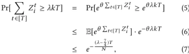
e Õt 2[T ]Zit · e k+34· 2k2N. Then, taking expectation and using the induction hypothesis com-pletes the induction proof. ⇤ L����5.7. Suppose N is an upper bound on the number of points stored by the data structure L at any time, and� x any i 2 [k]. For any 2, Pr[Õt 2[T ]Zit kT] e (
T N).
P����. Using the standard method of moment generating func-tion as in the proof of the Cherno� bound, we choose = 1
k N in the following: Pr[’ t 2[T ] Zit kT] = Pr[e Õt 2[T ]Zit e kT] (5) E[e Õt 2[T ]Zit] · e kT (6) e ( 7 4 )T N , (7)
where (6) follows from Markov’s inequality and (7) follows from Lemma 5.6 and the choice of = 1
k N. ⇤
The following theorem follows from Theorem 5.4 and Lemma 5.7. T������5.8. Let N be an upper bound on the number of points at any point in time (|Xt| N , for all t). For any > 0, for any sequence of T 2 N insert/delete operations the F����D��C���� algorithm maintains a (2 + )-approximation solution for the k-center problem. Moreover, the probability that the total time exceeds (log · k2T) is at mostlog · ke (NT), for any 2, under the fully dynamic
model. The algorithm requires O(log · N ) space.
1A random variable Z is stochastically dominated by a random variable Y if for all
real x, Pr[Z x] Pr[Y x].
6 EXPERIMENTS
All our experiments have been carried on a machine equipped with two Intel(R) Xeon(R) CPU E5-2660 v3 running at 2.60GHz and with 250Go of DDR3 SDRAM. The Twitter dataset we used as well as our implementation in C of our algorithm have been made publicly available2. Observe that for each tweet we retain only its timestamp and its GPS coordinates, due to privacy concerns. We evaluate the algorithms under a wide range of values for k, and the length of the sliding window W . In all experiments the default values are k = 20 and = 0.1, unless otherwise speci�ed. For our randomized algorithm, each result is the average among ten runs, unless otherwise speci�ed.
6.1 Datasets
We consider some datasets that are publicly available, as well as a dataset that we collected from Twitter.
Twitter. We collected geotagged tweets by means of the Twitter API. We were able to collect 21M tweets between 9/09/2017 and 20/10/2017. Each tweet is associated with GPS coordinates, such as longitude and latitude, as well as, a timestamp.
Flickr. The Yahoo Flickr Creative Commons 100 Million (YFCC100m) dataset3is a dataset containing the metadata of 100 Million picture posted on Flickr under the creative common licence between 2011 and 2015. Each picture is associated with GPS coordinate and a timestamp. We used the metadata of 47M pictures that possessed both a valid timestamp and GPS coordinate.
Trajectories. This dataset contains trajectories performed by all the 442 taxis running in the city of Porto, in Portugal4. Each tra-jectory consists of a set of two-dimensional points, each one being associated with a timestamp.Trajectories are updated every 15 sec-onds, with most of the trajectories consisting of at most 500 points. The dataset contains 83M two-dimensional points, in total leading to 83M updates.
Table 2 summarizes the statistics of the datasets considered in our experimental evaluation.
6.2 Distance Measures
Depending on the dataset at hand, we consider di�erent distance measures. In the case of Twitter and Flickr, we compute the great circle distance between two GPS coordinates [15]. For the trajecto-ries we use the symmetric Hausdor� distance [16], which is de�ned as follows. Let P and Q be two sets of points in the Euclidean space. H(P, Q) := max
p 2Pminq 2Qd(p,q) where d is the Euclidean distance. The symmetric Hausdor� distance between two trajectories P and Q is de�ned as bH(P, Q) = max(H(P, Q), H(Q, P)). All the distance measures considered in our experiments are metrics.
6.3 Dynamic Model of Computation
In the case of Twitter and Filckr, we evaluated the algorithms under the sliding window model [6, 7]. In this case, if a point is inserted at time t, it will be removed at time t +W , where W is the duration of
2https://github.com/fe6Bc5R4JvLkFkSeExHM/k-center 3http://yfcc100m.appspot.com/
4https://archive.ics.uci.edu/ml/datasets/Taxi+Service+Trajectory+-+Prediction+
Name Source Type #Updates Twitter twitter.com 2D points 42M
Flickr yfcc100m.appspot.com 2D points 96M Porto taxi trajectories archive.ics.uci.edu Trajectories 83M
Table 2: Dataset statistics.
the sliding window. As a result, at each point in time t, new points might be added to the current dataset in which case any point with timestamp t + W will be removed (if any).
We then focus on the task of maintaining a clustering of all trajectories available up to any given point. At any point in time, either a new point is added to one of the available trajectories at that time or a new trajectory is created. Since trajectories might be updated in any arbitrary order, the sliding window model turns out to be over-simplistic in this setting. Therefore the approach in [6] cannot be used.
6.4 Flickr and Twitter
We evaluate the algorithms under a wide range of values for k, and the length of the sliding window W . In all experiments the default values are k = 20, eps = 0.1. For Twitter, the length of the sliding window is two hours, while for Flickr it is six hours. Both those values result in a sliding window containing 60K points.
We start by evaluating the accuracy of the two algorithms. In particular, we measure the ratio between the maximum radius of the clustering produced by each algorithm and a lower bound on the optimum radius. At any point in time, we compute such a lower bound as follows. Let be largest such that the set U computed by our algorithm is not the empty set. Our lower bound is computed as half the minimum pairwise distance between the k + 1 points (cluster centers) in S . We observe that in practice it is important to have small maximum radius, in that, this might lead to more “meaningful” clusters.
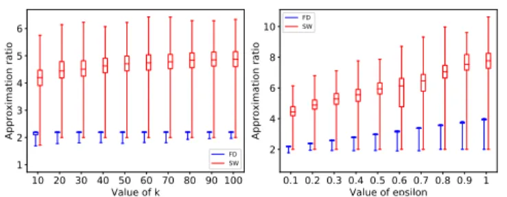
Figure 1 (left) measures the approximation ratio as a function of k, while Figure 1 (right) measures the approximation ratio as a function of in Twitter. For any given value of k and we report the median, the� rst and third quartiles, as well as maximum and minimum approximation ratio obtained by the algorithm when executed on the whole dataset. The two algorithms have been tested for the same value of k and , however, some additional space between the corresponding values in the plot has been introduced to improve the presentation.
We can observe that our algorithm (FD) consistently delivers better approximation ratio then the algorithm presented in [6] (SW). In particular, we can observe that while the approximation ratio of our algorithm is always close to 2 when = 0.1, it can be as large as 6 for SW with its median being as large as 4.5. This is expected, as our algorithm comes with stronger guarantees on the maximum radius. We can also see that on average FD performs better than its worst-case analysis suggests.
This is even more apparent in Flickr (Figure 3), where our al-gorithm produces results being closer to an optimum solution. In particular the median for the case when k = 100 and = 0.1 ((Fig-ure 3) (left)) is close to 1.5, while in a few cases a near-optimal
Figure 1: Ratio between the maximum radius and a lower bound on the optimum radius as a function of k (left) and (right) on Twitter. The two algorithms have been tested for the same value of k and , however, some additional space between the corresponding values in the plot has been in-troduced to improve the presentation.
solution is computed. We can also observe that the maximum ra-dius for SW drops as k increases, while it improves again when k is large enough (Figure 3) (left)). This might be due to the way the deletion of a center is handled in SW. If a center is removed, the cluster is not reconstructed as in our case but a new point (called orphan) might be elected as representative of the cluster. Although this might be more e�cient in practice, it might a�ect the quality of the results, in that, orphans might not be as good representatives of the clusters as the original centers. As a result, points might be added to the “wrong” clusters. As k increases, it becomes more likely that there is at least one “bad” orphan, which explains the drop in quality of the results. For even larger values of k, the task of clustering becomes “easier” with the easiest case being when k approaches the total number of points.
Figure 1 (right) and Figure 3 (right) show the approximation ratio as a function of for Twitter and Flickr, respectively. Those �gures con�rm that our algorithm produces better results in prac-tice. Moreover, we can see that the approximation ratio worsens as
increases, which is expected.
We then move to evaluate the average running time of the two algorithms, which is de�ned as the total running time of the al-gorithms divided by the total number of update operations. The expected running time of our algorithm has been studied in The-orem 5.4. Figure 2 shows the average running time of the two algorithms as a function of k (left) and as a function of (right) in Twitter, while Figure 4 shows the corresponding plots for Flickr. We can see that SW is consistently more e�cient than our algorithm, which is expected. However, both algorithm are very e�cient with the average running time being at most 5 ⇤ 10 4seconds and as small as 2 ⇤ 10 5seconds in some cases.
Figure 2: Running time of the algorithms in second as a func-tion of k (left) and (right) on Twitter.
Figure 3: Ratio between the maximum radius and a lower bound on the optimum radius as a function of k (left) and (right) on Flickr. The two algorithms have been tested for the same value of k and , however, some additional space between the corresponding values in the plot has been in-troduced to improve the presentation.
Figure 4: Running time of the algorithms in second as a func-tion of k (left) and (right) on Flickr.
6.5
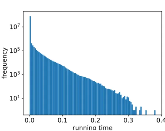
Trajectory Data and Multicore Implementation In this section, we consider the task of clustering trajectory data. We consider the scenario where at each point in time, either a new point is added to one of the existing trajectories or a new trajectory consisting of one single point is created. Each update can therefore be seen as either an insertion of a new trajectory or a deletion of an existing trajectory followed by an insertion of the updated trajectory. Since trajectories can be modi�ed in any arbitrary order, the sliding window model appears to be simplistic in this setting. Therefore, the algorithm in [6] cannot be used. TheFigure 5: Histogram of the running time of each operation during a single run on trajectories of our algorithm
distance between any two trajectories is computed as the symmetric Hausdor� distance (see Section 6.2), which is a metric.
Computing the distance between two trajectories requires (r) operations, where r is the maximum number of points in the two trajectories. In our dataset, most trajectory contain up to 500 points with the largest one containing nearly 4000 points. This makes the problem of clustering trajectory data more computationally extensive than in the case of two-dimensional euclidean space. Therefore, in order to be able to conduct an extensive evaluation of the algorithm, we consider a multicore implementation. Since the clusterings C ’s can be processed independently, a multicore im-plementation is straightforward: the C ’s are partitioned across the threads, with each thread taking care of all deletions and insertions in the clusterings associated to such a thread. All our experiments discussed in this section use 30 threads.
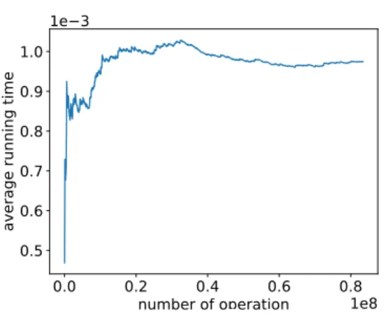
We� rst evaluate the running time of our algorithm. Figure 5 shows the histogram for the running time of each update operation (in seconds). In particular, for each running time value, the number of update operations requiring that running time is reported. We can see that approximately 80M operations require less than 4⇤10 3 seconds, while the maximum running time per operation is 0.38 seconds. Figure 6 shows the average running time as a function of the number of update operations. At any point in time, the average running time is computed as the total running time divided by the total number of operations up to that point. The running time is measured in seconds. We can see that the average running time is always less than one millisecond, while it becomes stable after approximately 18 million update operations. This is consistent with Theorem 5.8, which roughly speaking states that the probability of signi�cantly deviating from the expected running time becomes very low when the number of update operations is large.
As for the approximation ratio, using the default value of k and , we obtain a median of 2.05, while the� rst and third quartile are respectively equal to 2.03 and 2.13.
Figure 6: Evolution of the average running time per opera-tion during a single run
Figure 7: concentration of measure experiments
6.6 Concentration around the Expectation
Our last experiment aims to study the concentration around the expected running time (i.e. Theorem 5.8) from an experimental point of view. We consider 100 runs of our algorithm on the Twitter dataset using the default values and we show the histogram of the average running time in Figure 7. We can see that almost all runs require 5.8 ⇤ 10 4seconds on average, while in very few cases the average running time is more than 12 ⇤ 10 4seconds, which is consistent with Theorem 5.8.
7 CONCLUSION AND FUTURE WORK
In our work, we developed a (2 + )-approximation algorithm for k-center clustering, under a fully dynamic adversarial model of com-putation. In such a model, points can be inserted or deleted arbitrar-ily, provided that the adversary does not have access to the random choices of our algorithm. Our theoretical analysis, shows that the expected amortized cost of our algorithm is poly-logarithmic (in some cases of interest) while we show concentration around its expected value. Our work is the� rst work with strong theoretical
guarantees for fully dynamic k-center clustering, to the best of our knowledge.
We then conducted an extensive evaluation of our algorithm on dynamic data from Twitter, Flickr, as well as trajectory data. Our experiments show that our algorithm produces clustering solutions with smaller maximum radius in comparison with state-of-the-art approaches, although this comes at the price of slightly worse average running time and more space.
For future work, we are planning to study other data mining and machine learning algorithms under the fully dynamic model of computation.
REFERENCES
[1] R. P. L. A. Epasto, S. Lattanzi. Ego-splitting framework: from non-overalapping to overalapping clusters. In KDD 2017.
[2] D. Arthur and S. Vassilvitskii. k-means++: the advantages of careful seeding. In Proceedings of the Eighteenth Annual ACM-SIAM Symposium on Discrete Al-gorithms, SODA 2007, New Orleans, Louisiana, USA, January 7-9, 2007, pages 1027–1035, 2007.
[3] B. Bahmani, B. Moseley, A. Vattani, R. Kumar, and S. Vassilvitskii. Scalable k-means++. PVLDB, 5(7):622–633, 2012.
[4] M. Charikar, C. Chekuri, T. Feder, and R. Motwani. Incremental clustering and dynamic information retrieval. In Proceedings of the twenty-ninth annual ACM symposium on Theory of computing, pages 626–635. ACM, 1997.
[5] M. Charikar, L. O’Callaghan, and R. Panigrahy. Better streaming algorithms for clustering problems. In Proceedings of the 35th Annual ACM Symposium on Theory of Computing, June 9-11, 2003, San Diego, CA, USA, pages 30–39, 2003. [6] V. Cohen-Addad, C. Schwiegelshohn, and C. Sohler. Diameter and k-center in
sliding windows. In 43rd International Colloquium on Automata, Languages, and Programming, ICALP 2016, July 11-15, 2016, Rome, Italy, pages 19:1–19:12, 2016. [7] A. Epasto, S. Lattanzi, and M. Sozio. E�cient densest subgraph computation in evolving graphs. In Proceedings of the 24th International Conference on World Wide Web, WWW 2015, Florence, Italy, May 18-22, 2015, pages 300–310, 2015. [8] S. L. F. Chierichetti, R. Kumar and S. Vassilvitskii. Fair clustering through fairlets.
In NIPS, 2017.
[9] T. F. Gonzalez. Clustering to minimize the maximum intercluster distance. Theo-retical Computer Science, 38:293 – 306, 1985.
[10] S. Guha, N. Mishra, R. Motwani, and L. O’Callaghan. Clustering data streams. In 41st Annual Symposium on Foundations of Computer Science, FOCS 2000, 12-14 November 2000, Redondo Beach, California, USA, pages 359–366, 2000. [11] S. Gupta, R. Kumar, K. Lu, B. Moseley, and S. Vassilvitskii. Local search methods
for k-means with outliers. PVLDB, 10(7):757–768, 2017.
[12] S. Lattanzi and S. Vassilvitskii. Consistent k-clustering. In ICML, 2017. [13] M. D. M. H. S. L. M. Bateni, S. Behnezhad and V. Mirrokni. On distributed
hierarchical clustering. In NIPS 2017.
[14] R. Matthew Mccutchen and S. Khuller. Streaming algorithms for k-center clus-tering with outliers and with anonymity. APPROX ’08 / RANDOM ’08, pages 165–178, 2008.
[15] H. Steinhaus. Mathematical Snapshots. 3rd ed. New York, 1999.
[16] A. A. Taha and A. Hanbury. An e�cient algorithm for calculating the exact hausdor� distance. IEEE Transactions on Pattern Analysis and Machine Intelligence, 2015.
![Table 1: Summary of our algorithm (FD) and the one proposed in [6] (SW).](https://thumb-eu.123doks.com/thumbv2/123doknet/12402386.332156/4.918.179.749.125.184/table-summary-algorithm-fd-proposed-sw.webp)