Development of discontinuous Galerkin method for nonlocal linear elasticity

MASSACHUSETTS INS OF TECHNOLOGY

SEP

2 7 2007

Development of Discontinuous Galerkin Method

for Nonlocal Linear Elasticity

by

Ram Bala Chandran

B.Tech., Mechanical Engineering

Indian Institute of Technology, Madras (2005)

Submitted

to the The School of Engineering

in partial fulfillment of the requirements for the degree of Master of Science in Computation for Design and

Optimization

at the

MASSACHUSETTS INSTITUTE OF TECHNOLOGY

September 2007

@Massachusetts

Institute of Technology 2007. All rights reserved.

A u th or ... I... . ... The

School

of Engineering

July 6, 2007

Thesis

Supervisor

... . . . . . . . .

Professor Rad~l Radovitzky Department of Aeronautics ansl Astronautics

Accepted by ...

...

_...

_.

_{. . .-}

4

_....

_.

)

_.

_...

_..

Professor Jaime Peraire Department of Aeronautics and Astronautics t -irector, Computation for Design and Optimization Program

Development of Discontinuous Galerkin Method for

Nonlocal Linear Elasticity

by

Ram Bala Chandran

Submitted to the The School of Engineering on July 6, 2007, in partial fulfillment of the

requirements for the degree of

Master of Science in Computation for Design and Optimization

Abstract

A number of constitutive theories have arisen describing materials which, by nature,

exhibit a non-local response. The formulation of boundary value problems, in this case, leads to a system of equations involving higher-order derivatives which, in turn, results in requirements of continuity of the solution of higher order. Discontinuous Galerkin methods are particularly attractive toward this end, as they provide a means to naturally enforce higher interelement continuity in a weak manner without the need of modifying the finite element interpolation.

In this work, a discontinuous Galerkin formulation for boundary value problems in small strain, non-local linear elasticity is proposed. The underlying theory cor-responds to the phenomenological strain-gradient theory developed by Fleck and Hutchinson within the Toupin-Mindlin framework. The single-field displacement method obtained enables the discretization of the boundary value problem with a conventional continuous interpolation inside each finite element, whereas the higher-order interelement continuity is enforced in a weak manner. The proposed method is shown to be consistent and stable both theoretically and with suitable numerical examples.

Thesis Supervisor: Professor Rad'l Radovitzky Department of Aeronautics and Astronautics

Acknowledgments

I would like to thank my advisor, Prof. Raul Radovitzky, for his guidance, patience,

and support. I am also greatly thankful to my advisor for making my stay at MIT fun, challenging and for getting me into using and appreciating open-source software. I am thankful for the support of the DoE through the CalTech ASC Center for Simulation of Dynamic Response of Materials under contract 82-1052904.

I would always be grateful to my undergraduate advisors Prof. M.S Sivakumar and Dr. C.V.Krishnamurthy at IIT Madras for inspiring and making me believe that i am capable of doing research.

I am grateful to my program co-directors, Prof. Jaime Peraire and Prof. Robert

Freund for starting and running the most amazing program at MIT.

I would like to thank my graduate administrators, Laura Rose and Laura Koller for

essentially making me not worry about any paper work at MIT. My great appreciation to Brian, our lab administrative assistant for feeding me with Indian food during our group meetings.

I shall always be grateful to Dr. Ludovic Noels, University of Liege-Belgium,

for 'baby-sitting' me from time to time, for always being there on Yahoo messenger to help me out, and for being one of the most important source of motivation and inspiration at MIT.

Words would do no justice-to the help, motivation and of-course all the football videos ,espresso shots and loads of debugging help from my labmates, Dr. Antoine Jeruselam and Dr. Nayden Kambuchev. I am grateful to my labmates Sudhir and Ganesh for not eating my "Mexican-beauty" pizzas in the group meetings. I am thankful to all my office mates at building 41 for putting up with me for two years.

All this would not have been possible but for the sacrifices, encouragement and

motivation from my parents, my sister Rohini and my family back in India and in the US.

I would like to thank my friends at MIT - Ashish, Anshuman, Chetan, Deep, Dipanjan, Harish, Pranava, Sangeeth, Sandeep, Vikas and the entire sangam-brothers gang for making my stay at MIT fun and memorable.

Finally, I would like to thank my friends Adarsh, Krishna, Shankar, Srevatsan and Satyashree for suggesting to me that I cite their respective publications in atleast my acknowledgments and for being there when I needed you guys the most.

Contents

1 Introduction 13

2 A low order discontinuous Galerkin method for finite hyperelasticity 17

2.1 M otivation . . . . . 17

2.2 Discontinuous Galerkin formulation . . . . 18

2.3 Finite Element Implementation . . . . 24

2.4 Numerical Results . . . . 26

3 A discontinuous Galerkin formulation for linear nonlocal elasticity 31 3.1 Toupin-Mindlin strain-gradient theory of linear elasticity . . . . 31

3.2 Discontinuous Galerkin formulation . . . . 36

3.3 Theoretical stability and convergence . . . . 44

3.3.1 Consistency . . . . 44

3.3.2 Stability . . . . 46

3.3.3 Convergence Rate . . . . 49

3.4 Finite Element Implementation . . . . 50

4.1 Tension Test . . . . 4.2 Bi-material tensile test . . . . 4.3 Clamped Beam under bending loading 4.4 Size effects under torsion . . . .

. . . . 60

. . . . 61

. . . . 65

. . . . 68

5 Conclusions A Strain Gradient Constitutive Relations B Derivation of the upper bound of the bilinear form C Convergence Analysis- discontinuous Galerkin method D Implementation of second order derivatives of the element shape functions E Analytical solutions for 1-D strain gradient problems 73 83 85 91 95 99 E.1 Uni-axial tensile load . . . . 99

List of Figures

2.1 Convergence Analysis of the discontinuous Galerkin method applied to the cantilever beam problem in small deformation. The plot shows the error v/s mesh size h for 3 - 1.5, 3,15 . . . . 27

2.2 Convergence Analysis of the discontinuous Galerkin method applied to the cantilever beam problem in large deformation. The error in tip deflection E v/s mesh size h for # = 1.5,3,15 and the continuous

G alerkin case . . . . 28

2.3 Comparison of linear interpolation and quadratic interpolation for

dis-continuous Galerkin method for beta = 1.515 and continuous Galerkin

m ethod . . . . 29

3.1 Schematic description of the Body BO, and the discretization Boh . . 37

3.2 Interface Element with the two adjacent tetrahedra . . . . 54

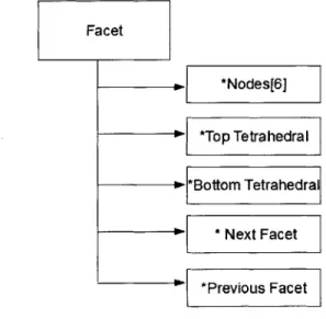
3.3 Data structure for Storing facet information . . . .. . . . . 55

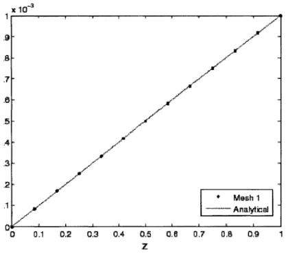
4.2 comparison of u; along z axis of mesh 1 in 4.4 subjected to an tensile load and the analytical solution for the unidimensional tensile load problem . . . . 61

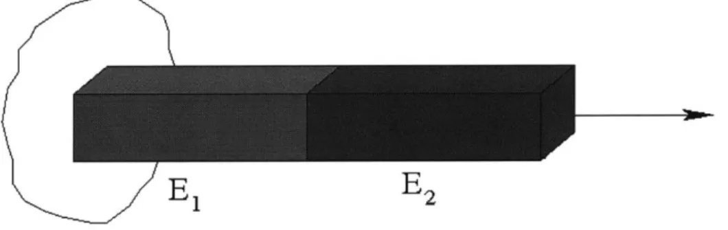
4.3 Bi-material tensile loading test . . . . 62

4.4 Tensile test problem discretization employed (a) mesh 1 ;(b) mesh 2; (c) m esh 3; (d) mesh 4. . . . . 63

4.5 Displacement profile for a bi material specimen subjected to tensile load 64 4.6 Strain profile for a bi material specimen subjected to tensile load . . . 64 4.7 Convergence analysis: L2 norm of the displacement error v/s mesh size 65 4.8 Comparison of numerical and analytical results of strain profile along

the z axis for three different values of .66

4.9 Bending problem illustration . . . . 67

4.10 Plot of stiffness ratio to the ratio of length of the beam to the length scale param eter . . . . 68

4.11 Description of the problem setup for torsional loading of a prismatic beam of square cross-section . . . . 70

4.12 An illustration of the mesh used in the torsion example . . . . 71

4.13 Plot of torsion stiffness ratio -y to the ratio of thickness of the beam to the length scale parameter . . . . 71

List of Tables

2.1 Geometric and material properties for beam bending problem . . . . 26

4.1 Tensile test material properties . . . . 61

4.2 Bi-material tensile test material properties . . . . 62

4.3 Bending test material properties . . . . 67

Chapter 1

Introduction

A number of constitutive theories have arisen describing materials which, by nature,

exhibit a non-local response. As-in, the stress at a material point is not just a function of strain at that particular point, as assumed in conventional theories, but also a function of strain in its local neighborhood, leading to the name non local or strain

gradient theories. Cosserat, first proposed the couple stress theory , where in addition to the displacement u an independent rotation quantity 0 is also defined. The couple stresses are then introduced as the work conjugate of spatial gradient of 0. Later Toupin [29] and Mindlin [30, 20] proposed a general theory theory which took into account not only micro-curvature but also gradients of normal strain. The initial theories proposed were for linear elastic materials. Later, several theories have been developed to take into account plastic flow theories (Fleck and Hutchinson[10, 22], Anand et al. [17]), crystal plasticity, crack growth (Smyshlyaev [38]) and several other microscopic behaviors exhibited by materials [19, 39, 37].

gradients, leads to a system of equations involving higher-order derivatives which, in turn, makes the problem hard to solve both analytically and computationally. Computational difficulties arises in the solution scheme owing to the presence of higher order derivatives which in-turn require the solution field to be at least C'

continuity over the solution domain i.e. both the displacements and the first order derivatives should be continuous along the inter-element interface.

Zienkiewicz and Taylor [28] introduced a C' continuous element, but its shape and the number of degrees of freedom needed per element puts serious limitations on its usability and scalability. A mixed type elements have been previously proposed, where at each node apart from the displacements an extra rotation angle 6 [41, 15, 16] or the couple stress is stored as nodal DOF. More recently, meshless Galerkin methods has been applied to problems with strain gradient effects in two dimensions.[14, 35]. Standard patch tests and benchmark problems have been tested on some of these methods, but rigorous mathematical proofs of rate of convergence, consistency and stability have not been demonstrated.

Discontinuous Galerkin methods are particularly attractive toward this end, as they provide a means to naturally and in a consistent way to enforce higher order inter-element continuity in a weak manner. Discontinuous Galerkin methods where first developed to solve neutron transport problem [33], has now been successfully applied to solve numerous elliptic and hyperbolic problems occurring in fluids and solid mechanics.[2, 8, 6, 36, 25, 27, 18]

In the context of elliptical problems Brezzi et al. [6] proposed a discontinuous galerkin method to solve the scalar poisson equation. Arnold et al. [1] presented a

detailed study of DG methods for second order elliptic equations. With the con-text of higher order elliptic equations Engel et al. [8] proposed the continuous-discontinuous(C/DG) Galerkin method, where the displacements across element in-terfaces are continuous whereas the jump in derivatives are penalized to impose

C' continuity across the elemental interface. They proposed a C/DG formula-tion and implementaformula-tion in one dimensions for Bernoulli-Euler beam bending and Toupin-Mindlin strain gradient theory, and a formulation and implementation in two-dimension for poission-kirchoffs plate theory. This sparked several related work toward's development of discontinuous galerkin methods for plate,shell theory prob-lems and damage probprob-lems [40, 21]. Discontinuous Galerkin method has been devel-oped for Reissner-Mindlin plates [2], Timoshenko beams [7], shells [12, 11] and for Kirchoff-Love shells [24]. Susanne et al. [4] developed rigorous stability and conver-gence results for a continuous-discontinuous galerkin method motivated from Engel

et al. [8] toward's solving scalar fourth order elliptic equations in two-dimensions.

In this work, a discontinuous Galerkin formulation for boundary value problems in small strain, non-local linear elasticity is proposed. The underlying theory cor-responds to the phenomenological strain-gradient theory developed by Fleck and Hutchinson [10] within the Toupin-Mindlin framework. The single-field displacement method obtained enables the discretization of the boundary value problem with a conventional continuous interpolation inside each finite element, whereas the higher-order inter element continuity is enforced in a weak manner. The proposed method is shown to be consistent and stable both theoretically and with suitable numerical examples.

In Chapter 2, the formulation and numerical examples of discontinuous Galerkin method for finite hyperelasticity with emphasis on alleviating the problem of locking which arises in low order finite element interpolation schemes. In Chapter 3, the formulation, analytical properties and finite element implementation of discontinuous Galkerin method for nonlocal linear elasticity is presented and to conclude in Chapter 4 results, conclusions and recommendation for future work are made.

Chapter 2

A low order discontinuous Galerkin

method for finite hyperelasticity

2.1

Motivation

It is well established numerically and analytically that a higher order scheme have a better convergence rate when compared to lower order schemes [28]. However the advantage of a low order scheme is that it is relatively less expensive than the higher order schemes. Elements which employ linear interpolation are by far the most used and computationally an inexpensive method to get an approximate solution. When it comes to modeling incompressible materials and plasticity, finite element method exhibits locking [13]. In a conventional finite element method, this leads to decrease in convergence rate. It is also well established that the effects of locking are more prominent in linear elements in comparison to quadratic elements [13]. Several meth-ods have been proposed to alleviate the problem of locking including mixed

formu-lation [9, 34], under integration [28] and they work very well. In this work we try to demonstrate one of the several advantages of employing a discontinuous Galerkin formulation developed for non-linear elasticity [25] intrinsically avoids the problem of locking. We choose a linear tetrahedral element, so as to clearly demonstrate that a discontinuous Galerkin formulation clearly eliminates locking. Firstly, we develop the discontinuous Galerkin formulation based on the work of Noels et al. [25, 26], where the discontinuous galerkin formulation is derived from the weak form, secondly dis-cuss some of the implementation issues and finally numerical examples are presented towards this end.

2.2

Discontinuous Galerkin formulation

The governing equations along with the boundary conditions for a large static defor-mations of elastic bodies in equilibrium is given by,

VoP + poB = 0 in Bo (2.1) p = p on aDBO (2.2)

P.N= Ton &NBO (2.3)

where, Bo C R' is the region occupied by the body in its reference configuration, P is the first Piola-Kirchhoff stress tensor, poB represents body forces per unit reference volume, Vo is the gradient operator in the reference frame, p is the corresponding deformation mapping of the deformation of material particles, N is the unit normal

to the surface in the reference configuration and : and T are the boundary conditions applied on the displacement ODBO and traction &NBO parts of the boundary,

respec-tively. Also, its worthing noting that, aBO = aDBO U ONBO and &DBO n aNBO = 0

For the constitutive law a general class of hyperelastic material models are con-sidered for which stress can be computed from a strain energy density function

W = W(F) given by:

P aw (2.4)

aF

where, F = Vop is the deformation gradients. As a direct consequence of Material

frame indifference it can be easily shown that the strain energy density function W depends only on the right Cauchy-Green deformation tensor, that is W = W (C) and where C is given by FTF.

The first step towards the development of a discontinuous Galerkin formulation is discretization of the BO into smaller domains Q' such that

E

BO ~ BOh =JQ (2.5)

e=1

Here E is the total number of sub-domains present in the body, e is an index which runs over all the elements and Boh an approximation for Boh represents the the body the union of Q' represent. Since mesh generation, inter element interpolation

and integration schemes are well developed for conventional finite element meshes (Tetrahedral & Hexahedral in 3-d), we are going to consider a decomposition of BO into tetrahedral elements (Q') for implementation purposes. But the mathematical

formulation presented in this section will hold good for any type of domain decompo-sition. Let subscript I correspond to the boundary between two sub-domains. Then

a = &DQ₀ U _{&NQ 0} U OI and &IBOh = E ₁ Q \&B Once the domain has been

decomposed, the appropriate spaces for the test and trial functions have to be chosen in order to construct the solution. In a discontinuous Galerkin method we allow for discontinuities in the solution space along the internal surfaces (OIBoh). That is, the field variables and the test function can have a jump along the interface of any two elements. Now, like in any finite element formulation it is essential to introduce a finite-dimensional piecewise polynomial approximation ph, 6Wh for the displacement

field W and test function 6W at all points inside the body Boh which exist in the following spaces:

Xkh Ph C L2 _(Boh)

I

_{[IhlEpk(Q) V'EBOh} (2.6)}

with Xk = {6 X (2.7)

The weak form of equilibrium equation (2.1) is obtained by multiplying equation with a test function (6p,), and integrating in the domain _(Boh).

E E

Sf

6ph? hdVo

±+

f

6hpoBdVo = 0 V 6w E (2.8)

Integrating the first term of equation(2.8) by parts E E - jPh: VhdVo + E I ah - Ph -NdSo e 90 e 0 E + E jhpPoBdV V 6p ( Xc e 90 (2.9)

We now separate the internal boundary terms(&iQ8) and the external boundary terms(aDQe U &NQe) in (2.9) using Neuman boundary condition (2.3) and from the

definition of the test function space Xc (2.7) leading

to-E 0 = - Eo E Ph VO&PdVO ₊

_E

_n 6Wh - Ph -NdSo E + i aenaOGNBo Ph 'TdSO+ 6WhpOBdV V e 0B

It is appropriate to introduce the jump

[9]

and the mean

(.)

operators defined on the space of functions which can have multiple values on the interior boundary

TR(aIBOh) = He1 1 (L2(9,1Q))

] , (e) : [TR(&IBoh)]i or 2 _ [L2(IBOh)] 1 or 2 _I] ,+ _,-, (0 __ [.+ +

0-(2.11) In above expressions, the bullet represents any field,

.±= lim 0 (X ± eN-)

6-0+ V X

c

&IBoh

and N- is the outward normal of aQe. The primary idea of discontinuous Galerkin (2.10)

6 _{p E Xk}

(2.12)

method is that, we allow for discontinuity on Ph and 6 _{h along the elemental interface} QIBho. The discontinuity along internal element interface is written as a flux term

[26].

E

1

L

o

6Wh -Ph -NdSo -+ - [6jhp -h

(P-,

P+, N-) dS (2.13)

e Qnj B Oh 'I0 8BOh

where, h (P-, PI, N-) is the inter-element flux term. Although we have an option in choosing any arbitrary flux term, in order to satisfy consistency of the weak for-mulation the flux should atleast satisfy the following properties [26].

h(P,P,N) = P-N (2.14)

h(P, P, N-) = -h(P ,P-,N+) (2.15)

Using equation(2.13), equation (2.10) can be expressed as:

E

0 = - Ph: VOWOhdVO -

j

o6 Wh -h

(P-,

Pi, N-) dSo

E E ('6

+ 1Jn:NBO S ' TdSO SIhpOBdV V 6(p E Xh

The stability of the weak form depends on the choice of flux. A wide repertoire of fluxes have been listed and their stability and convergence issues have been discussed

been numerically and analytically demonstrated by Noels et al. [25]

h (P-, P+, N-) = (Ph) -N- + 1 9 N-.

K+CI

- ON- (2.17)

where C is the mean tangent stiffness at the interface,

Q

is an appropriate stability parameter chosen such that the scheme is stable and h, is the characteristic length of the mesh

= min

(

(2.18)

hS

q&Qe-

V

e+

substituting (2.17) into the weakform (2.16), we get

0 = jP : V OdVo - ' ' -6WdSo

J Oh " BOh

+

Di6

-

(P)

-N-dS

0

+

[oh ]

N-

C . h[] N-dSo

aj BOh aj BOh h

(2.19)

This is the final form of the discontinuous Galerkin formulation for non-linear elas-ticity. The stability, consistency and convergence of the above formulation is shown in Noels et al. [25]. This formulation also exactly corresponds to whats known as the

Interior Penalty method. We have essentially derived the same formulation using the

2.3

Finite Element Implementation

The weak form as obtained in equation (2.19) can be easily implemented with little effort into a regular finite element code. Essentially the first two terms in the right hand side of equation (2.19) correspond to the terms arising from a standard Galerkin formulation. In order to perform integration over the internal surface an interface element very similar in notion to the ones used in cohesive elements for fracture is introduced [25]. A Newton-Raphson based solution procedure is setup to solve the system of non-linear algebraic equations given by

fint(x) + f'(x) = fext(X). (2.20)

Here fint is the internal force contributions that come from each volume element and is expressed as

fj"l _a = P.Na,xdV, (2.21)

e

f'(x) is the interal force contributions from the interface elements and is expressed

as

falI = / (P) -N-NadSo

N-IB~

(2.22)

I

-- CK

:

Xb] 0 N- N-NaNdSo

JaIBOh Ih C

At each iteration a linearized form equation (2.20) is solved and the nodal displace-ments are updated. The linearization of the left hand side of equation (2.20) results

in the tangent stiffness matrix (K'-) given as .

ntfint + fI')

Kiakb = _(Pa Jia) (2.23)

&Xkb

Rewriting equation (2.20) using the tangent stiffness matrix we obtain the linearized balance equation and the update equation.

K'-1AU = fext - (fiil + f;-1) (2.24)

U = UN1 + AUi (2.25)

Finally, in order to solve equation (2.24) we must compute the tangent stiffness of the

system. we only present the stiffness terms that arise from the interface terms, the volume term being straightforward. We first make an approximation of the stiffness matrix contribution arising from the internal interface terms. From (2.19) its clear that the forces depend on the stresses and the material moduli. Therefore the stiffness matrix involves all the degrees of freedom of the two adjacent tetrahedral. But for

large values of 3 the displacement jumps are small, therefore the stiffness term arising

from the stress term is going to be very small [25]. Using this approximation, the interface stiffness matrix is given as:

with a plus sign for the combinations + y+ and - i- and with a minus sign for other combinations. This approximation helps us to simplify the implementation but at the time the stability of the scheme is not affected [25].

2.4

Numerical Results

In this section we will demonstrate with the help of a beam bending problem that even a linear tetrahedral at nearly incompressible poisson's ratio does not exhibit locking. In this calculation the material model corresponds to a NeoHookean model extended to the compressible range. The strain energy density function given as follows

W= (log J- ) logJ+ 11 (1 -3) (2.27)

where A and y are the material parameters, J = det ((F)) and I, = tr(C). The

material parameters and the geometric characteristics of the beam used in calculations are listed in Table (2.1). In order to study the stability and convergence of the method

Table 2.1: Geometric and material properties for beam bending problem

Properties values

Length L = 1m

Height h = 0.1m

Initial Young modulus Eo = 200GPa

Initial Poisson ratio vo = 0.4999

in the first example we consider a prismatic beam with uniform cross-section whose geometric and material properties are listed in Table 2.1. The beam is clamped rigidly at one end and a force of 1OkN applied at the other. Using classical beam theory

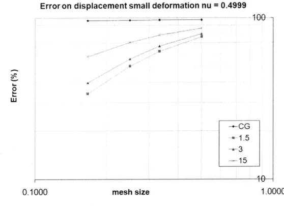
U-the tip deflection 6 = 4(L3/h4_{)(F/Eo) is computed to be 2mm. The error in the} tip deflection between numerical solution and analytical is plotted as a function of mesh size for three different values of 3 and is compared with the continuous Galerkin case. The tip displacement error remains a constant in the continuous Galerkin case,

Error on displacement small deformation nu = 0.4999

-0t LI -+-C 1.5 3 15 10 0.1000 mesh size 1.0000

Figure 2.1: Convergence Analysis of the discontinuous Galerkin method applied to the cantilever beam problem in small deformation. The plot shows the error v/s mesh size h for / = 1.5,3,15

whereas the error decreases with a slope equal to one for the discontinuous Galerkin formulation. The stabilization parameter 0 has no effect on the rate of convergence, but for a large value of

/,

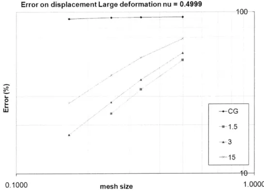
the solution becomes less accurate and approaches the continuous Galerkin solution. The same' convergence behavior is demonstrated for large deformations as well. To demonstrate the convergence behavior under large deformation's we consider use the same boundary value problem as described for

the small deformation bending problem but a load of 1MN is applied on the right face, perpendicular to the length of the beam. In order to compute the error, we assume the fine mesh solution obtained using a quadratic element in a discontinuous Galerkin formulation to be the accurate solution and the error is computed with respect to this value. Figure (2.2) shows a very similar convergence pattern as to

Error on displacement Large deformation nu = 0.4999

UCG

3

15

10

0.1000 mesh size 1.0000

Figure 2.2: Convergence Analysis of the discontinuous Galerkin method applied to the cantilever beam problem in large deformation. The error in tip deflection E v/s mesh size h for

#

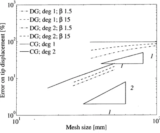
= 1.5, 3,15 and the continuous Galerkin case

the small deformation bending convergence. A comparison of the rate of convergence for linear and quadratic elements is studied for two different values of stabilization parameter / and for the continuous Galerkin formulation. From Figure (2.3) it is evident that for the same mesh size the quadratic elements have higher accuracy and

-- DG; deg 1;

1.5

-- DG; deg 1;4 15

-- DG; deg 2; [ 1.5

--- DG; deg 2;$ 15

CG; de

CG; dc

~g 1 - --.

-.g2

g22

10

102

Mesh size [mm]

Figure 2.3: Comparison of linear interpolation and quadratic interpolation for

dis-continuous Galerkin method for beta = 1.515 and continuous Galerkin method

also the fact that the rate of convergence is higher for the quadratic elements when compared to the linear elements. To conclude., discontinuous Galerkin formulation does not exhibit locking and the convergence rate is not affected by Poisson's ratio.

10 2

101

EV

Chapter 3

A discontinuous Galerkin

formulation for linear nonlocal

elasticity

3.1

Toupin-Mindlin strain-gradient theory of

lin-ear elasticity

In this section we present the linear elastic strain gradient theory developed by Toupin

[29] and Mindlin [30]. In this theory the strain energy density function W per unit

volume depends on the symmetric small strain measure ij = - (ui,j + ujj) and the

the form as given in equation (3.1)

W = W (Eij, r1ijk) (3.1)

The Cauchy stress o-ij is the work conjugate of the strain measure Eij whereas the higher order stress measure Tijk is the work conjugate of the higher order strain

measure Tijk and following from (3.1)

o w

(3.2)

aegy

Tijk =

(3-3)

a 0 _lijk

By employing the idea of virtual work the governing equations and the essential

boundary conditions can be obtained in strong form [29, 30, 10]. Following the same procedure as shown by Fleck and Hutchinson [10], the internal virtual work statement can be written as

6W dV = B(O-j6Eij _{+ ijki77ijk) dV}

JBO bk6udV +

j

N UdS + JMB TOUk,lfnldS

where, ONBO corresponds to the boundary where traction tk is specified, aMBO corre-sponds to the boundary where double stress traction Tk is specified and bk is the body

nat-ural boundary conditions of the problem and the corresponding essential boundary conditions are the displacement ik specified on the surface &DBO and the gradient of displacement projected along the normal to the surface niUk,i on the surface &TBO. It is worth noting that ONBO U ODBO = 9BO, 9NBo n 9DBo = aMBO U &TBO = Bo

and BBo n 9TBO = 0.A schematic description of the different boundary conditions

is illustrated in figure (3.1). Applying Gauss divergence theorem to the internal work terms in equation (3.4), we obtain

f Bo (Uij6Eij + Tijk6?ijk) dV = - B0 (Oik - Tijkji 6ukdV + J B0ni (Oik - TijkJ) 8ukdS

+ InfTijk6Uk,idS

JaBo

(3.5)

Here in equation(3.5), aBo is the surface of the body, ni is the unit normal to the surface of the body. However its worth noting that SUk vanishes at all points on the

surface aDBO, reducing equation (3.5) into

J BOJ (Uij6Eij + Tijknijk ) dV - B0 (9ik - Tijkjg 6UkdV + a NBoni (cik - TijkJ) 8ukdS

+ J njijkSUk,idS JOB0

(3.6)

It has to be noted that 6

Uk,i is not independent of of 6

Uk on the surface(&Bo) of Body

(B) [10, 201. So, in order to correctly identify the boundary conditions the gradient

normal gradient component, niD6uk and the surface gradient component, Dj6

uk.

6_{Uk,i = (}6

il - nini) (Uk),j + nin (uk),

(3.7)

= Dj6Uk + nfD6Uk

substituting equation(3.7) in equation (3.5)

(0-ij oers+ TijkOrjk) dV = - (O'ik - 'Tijk,j)i 6ukdV +

LNBo

ni (Uik - Tijk,j) SukdS

+

j

njTijk (6il - ning) 6Uk,ldS +

8BO I&Bo

njTijknjnf6Uk,jdS

(3.8)

The surface gradient term on the right hand side of equation (3.8) can be further simplified using integration by parts1 _{and followed by applying the surface divergence}

theorem2 .

I

BOnjTijk (61 - nini) 6Uk,dS

(6j - nini) (nfjrijk6Uk) ,j dS

-JBo

(Jim - ninm) ni,,m (njniFijk) tUkdS

(6i1 - ninl) (nrijk) ,1 6UkdS

- I (6il - ninl) (njTijk) ,1 6ukdS

'8BO

It should be noted in equation (3.9), that 3

Uk will vanish on the surface e3DBO and

in equation (3.8) 6

Uk,lnl vanishes on 9TBO, thus from equation (3.9) , the internal

'0 : Vov V= .(O.v) - (V'.4).v where VWis the surface gradient operator

Vf,V8. (O.v) dS = f₈ (V8.n) n.$.vdS [30]

3

It is noted here that the surface is assumed to be smooth and that there are no edges. =

_lB

0

=

_LB

0

virtual work terms now become (oijEEij + TijkJrlijk) dV

(Jim - ninm)rni,m(

ik ~ Tijk,j)i JUkdV + ni (rik - Tijk,j) 6UkdS

BO JaNBO

(njniTijk) 6ukdS -

INBO

(6ji - nini) (njTijk) , 6ukdS

ONBO

+

f njTijknjnl6Uk,1dS

(3.10)

using equation (3.10), the principle of virtual work equation (3.4) , is satisfied if the following local conditions hold true:

0 = 6k + (cxik - Tjik,j),i (3.11)

which represents the governing differential equation in strong form

(3.12)

is the traction boundary condition on the surface &NBO and

k ninjTijk (3.13)

is the applied double stress traction rk on DBM. It is assumed that the body has a smooth surface 9BO so that there are no edges, since the presence of edges will result in an additional integral term over the edge [10]. The governing balance equation (3.11) can be uniquely solved along with the six boundary conditions in (3.11) and (3.13) if

tk = ni (uik - ajTijk) + ninjijk (Dpnp) - Di (njFijk)

+

the strain energy density function used is convex with respect to both Eij and ?7ijk [22].

The boundary value problem resulting from the virtual work statement correspond to the non local linear elastic theory proposed by Toupin [29] and Mindlin[30], which can be summarized as follows

0 = bk + (Uik - Tjik,j) in BO (3.14) (9W aij= -

_a~ij

in BO (3.15) 8W Tijk = W in BO (3.16) 197]ijk 1

6ij= (ui,j + uj,j) in Bo (3.17)

tlijk = Uk,ij in Bo (3.18)

tk = ni (Jik - OjFijk) + nirijjk (Dpnp) - Di (nrijkT ) on aNBo (3.19)

rk - ninjTijk on iM Bo (3.20)

Uk = ukon aDBo (3.21)

niUk,i = Duk,i on 9TBO (3.22)

In the next section we will develop the discontinuous Galerkin formulation for the

boundary value problem described by equation (3.14, 3.19, 3.20 -3.22) and establish

stability and convergence properties.

3.2

Discontinuous Galerkin formulation

The preceding formulation of the boundary value problem in strong form is taken as a basis for the formulation of a discontinuous Galerkin weak form approximation

2 3

noMvo

Bo

c)DBo

Figure 3.1: Schematic description of the Body BO, and the discretization Boh

within the context of a finite element framework. The fist step in the development of a discontinuous Galerkin formulation is the decomposition of the domain (Bo) into

smaller sub-domains (Qe) such that Ue 1 Qe = Boh ~ Bo. As the mesh size (h) is

decreased, the body modeled by the meshes becomes closer to the actual geometry of

the body. The next step is to define the spaces for the trial (Uk) and the test functions

(W), which are C' continuous

{Uh C CO (Boh) c L2 _{(Boh) IUkhI}

EPk(Qe) VeB} C UI (Boh) (3.23)

Where Uf (Boh) = le H2 _{(Qe) for k > 1. It should be clear that this choice of}

between elements & = [ueE~iaQe]5 . The corresponding constrained space for the

test function is

U = {U E UC5UgaBO} C Uf (B.) (3.24)

U = {U E U1u6Ia=BO} (3.25)

We start with the equilibrium equation (3.14) and multiply with a test function

wE ULf and impose equilibrium in a weak sense

E

Wk (bk + (Jik - Tjik,j),) dV = 0 V w E Uf (3.26) e=1 e

From now on it will be assumed that the test functions belong to the constrained space (3.24). Applying integration by parts followed by Gauss divergence theorem

E E E

E

J

Wk (Jik - Tjik,j) nidS - Wk,iikdV - k,ijjikd

e=1 e=1 e e=1 e(3.27)

E E

+

Wk,iTjrinjdS +

E

j

WkbkdV = 0

e=1 Qea e=1 D

The integrals over the boundary of each element(0Qe) can be written as a summation of integrals over the internal interfaces and a summation over the external boundaries

E E E

E i~ ena~ Wk (Jik - jik,j) ridS - Ij Wk,iOikdV - Wk,ijTjikdV

e=1 e=1 e e=1

E E E Wk,ijikfjldS + L WkbkdV + Wk,iTjiknjdS e=1 e =1 e e=1 E + i Wk (Jik - Tjik,j) n dS = 0 e=1 (3.28)

Now defining a jump operator

[*]

= + - e- and a mean operator (e) = (+ + e--),

the first term of equation (3.28) can be expanded as follows.

E

e=1 gQngQIC

Wk (uik ~ Tjik,j) ridS= -

j

(jik k+ - TFjik,j) n$ + wk (Jik - Tjik,j nT) dS

J

Wk (ck - Tjikj) n dS

= - TWk1I (Jrik - T-jik,j) ry dS

- (Wk) T~ik - Tjik~J1 ri dS

(3.29)

where . denotes quantities on either side of the interface element, n- is the outward normal of the bottom tetrahedron. Here we have used the fact that on the interele-ment interface n- = -n+, the definition of the jump and mean operator and using the relation [abj = [a (b) + (a) [b]. The last term in equation (3.29) can be neglected because only compatibility of displacements needs to be enforced. In the first term

[Wk

= 0,since the space of interpolation and trial functions are assumed to be CO continuous in the whole domain (3.24). The second interelement boundary term in

equation (3.28) can be written as: E e=1 '90enaQC Wk,iTjikn dS

_=+wkn+

_kiTJ.kn) = - [Wk,iTjikj njdS

=

j ()

k~i Tji n S ~ (Wk,i) Tjikj -dS

J W~ (rjik ni _n

(3.30)

The last term of equation (3.30) can be neglected because only compatibility of dis-placement gradients needs to be enforced. The mean higher order stress (Tjik) can be expressed as a flux term 'rjiki- following the work of Brezzi et al. [5, 6] , Arnold et

al. [1], Noels et al [26].

E

z

J

Wk,iTjiknjdS ~~ - j wJ dS

e=1 gQ7ne aij Q

(3.31)

Inserting equation (3.29), (3.30), (3.31) into equation (3.28) we obtain

IWk]Tikl JdS

E Wk,igikdQ + E 1 Wk,ijjikdQ +

- j Wk (Uik - -bjikj) bi=dS

-jWk,i (Tiknj) dS -

le

WkbkdQ

=

0. (3.32)

For the sake of convenience the superscript on the normal is dropped, but it should be noted that when we refer to the normal of an internal surface, it corresponds to the outward normal of the oriented interelement boundary surface. Following the

procedure established in the previous section, the boundary integral terms occurring on the boundary OQ in equation (3.32) can be written as.

j

Wk,i (Tjiknj) dS +

J

Wk (o9ik - '7jik,j) nidS

=

j

Wk [ninjTijk (Dpnp) - Dj (nriTijk) + (uik - Tjik,j) ni] dQ (3.33)

+

I

niTinjfWk,InIdQ

From the first term in the right hand side of the first term in equation (3.33),

fa Wk (ninjTijk (Dpnr) - Dj (niir jk) + (9ik - Tjik,j) ni ) dQ constitutes the weak

enforce-ment of the traction boundary condition tk. The conjugate of this traction condition is the displacement (Dirichlet) condition. Since the displacement boundary condition can be enforced strongly, this term reduces to an integral over the Neumann boundary

(ONBo). The second term in the right hand side of equation (3.33) faQ niTjikriwk,inIdQ

constitutes the weak enforcement of the higher order traction boundary condition Tk

and its conjugate boundary condition is the normal component of the displacement gradient (njuij = Dui) on the surface. In the single field displacement method

pro-posed, displacement gradient cannot be specified independently and therefore higher order Dirichlet boundary condition need to be enforced weakly. Which is equivalent

of imposing a boundary flux term rjikrlj on &TBO. It is also worth noting that the

The boundary terms now are given by

Wki (riknj) dS +

I

Wk (uik - Tjik,j) nidS

Wk (nlrijTjk (Dpnp) - Dj (nriTjk) + (Uik - TJik,j) ni) dQ

niWk,lfnTjikfjdQ + rkWk,jnfdQ

{OaM

niWk,inlji kjdQ + rkWk,lindQ

=

WktkdQ

+

ON STC JM

Substituting equation (3.34) into the weak form we obtain

I: Wk,iUikdQ

+

If

Wk,igjTjikdQ

+

WktdS -

LTQ

niWk,lnlITjjkdQ

-f

QWkij [ TiiknjdS

(

TkWk,jnIdQ

-El

WkbkdQ =

0

e O (3.35)

We will now direct attention towards the definition of the flux term in the discontin-uous Galerkin formulation. The flux term will be defined such that the discontindiscontin-uous Galerkin formulation is consistent and stable. Following [25], first we define the nu-merical flux on the internal surface 042 as

Tjiknlj = (Thik) nj + nj

K

) Up,qj nr

where 3 is a stabilization parameter and h is the characteristic length of the mesh.

h =min ( I _0_1__l

e-QIVI

&gge+)

=

LT&.

+ fa

(3.34) - IN (3.36) (3.37)

The flux term on the external boundary aTQ is given as

I3Jjikqrp (.8

7-jiknj = Tjiknn + nj h (nsup,snq - Dupnq) nr (3.38)

and h on the external boundary of the mesh is given by

|Ge|

h = (3.39)

here Dup is the externally specified normal component of the displacement gradient. It is interesting to note that the idea of imposing boundary conditions in a weaksense was introduced by [23]. This flux term is similar in notion to the average flux introduced

by Bassi and Rebay [3] for fluids and the stabilization term is of the quadratic type.

Inserting the specific form of the flux term into the equilibrium equation we obtain the stable discontinuous Galerkin formulation for nonlocal linear elasticity

0 =

( WkiikdQ

+

WkjTjikdQ - WktkdS - e WbkdQ

e e e eJN Qe De

+

f

W,j [riik) nj + n

<

q T p,

nr

dS - Wk,lnrtlkdS

JaI0 h .IaM

- Wklnhlj [Tiknj + n h (nupsnq - Dupnq) nrIj dS

V Wk E Uf (3.40)

Equation (3.40) is the final weak form of the nonlocal linear elasticity problem along with the Dirichlet boundary condition ui = 7i on &DBO which is enforced strongly. In the next section, the theoretical stability and convergence properties of the

discon-tinuous Galerkin method will be demonstrated.

3.3

Theoretical stability and convergence

In this section we will demonstrate that the discontinuous Galerkin formulation for non local elasticity has the necessary properties essential for numerical convergence. The consistency and the stability of the method as well as the convergence rate are demonstrated.

3.3.1

Consistency

Let us consider the exact solution to the physical problem u E H2_{(Bho) . In particular,}

this solution belongs to C'(Bho), therefore one has the following

properties-kj = 0 on DiBo (3.41)

?7ijk = Uk,ij in Bo (3.42)

Applying Gauss divergence theorem to equation (3.40) and using equations (3.41, 3.42, 3.43 we

obtain-I

kbkd + QkhkdS + Qk,ln kdS + iTQ Wk,lhlJ'ini h i sup,snqmrdS

-aQ WkiknidS -

LOh

WkUik,idQ +

j

Wk,iTjiknjdS -

j

Wkjik,jnidS

--

j

k,i (Tjik) 'ijdS + Wk,ijTjikdQ +

j

Wk,i j (Tjik) 'jdS

J

Q 3 J BOh fQ

+ Wk,inininj h sup,snqnrdS

(3.44) In the above expression, canceling the interelement jump term, decomposing the boundary terms in the right hand side into mutually independent conditions as we did in the previous section and taking into account the spaces to which the test functions belong, we obtain

J kbk + NQ Wk (tk - ik) dS +

Lm

Q Wk,inl (rk - k) dS

+ Wk,l'Tfiii'j (nsup,s'nq - rsitp,snq) nrdS (3.45)

From the above equation it is clear that the strong form of the equilibrium equation is recovered, thus showing the consistency of the scheme.

o

= bk + (ujk - Tjik,j),j in Boh

tk = ni (cik - 9j7ijk) + ninj7ijk (Dpnp) - Di (njTijk) on &NBO rk = ninTijk Pls = nsP,s on O9MBO (3.46) (3.47) (3.48) (3.49) consistency leads to orthogonality, As the formulation is consistent, the exact solution (u) will also satisfy equation (3.45), therefore we have

a (Uh - U, 6u) = a (Uh, 6u) - a (u, 6u) = a (uh, 6u) - b(6u) = 0

3.3.2 Stability

Before we proceed to analytically demonstrate the stability of the proposed numerical scheme it will be necessary to define an energy norm I|| e I| : UIf (Bo) -+ R+

IIV 12_ - 22 = VCij klVk,l 2 + VJijklmnVn,lm 2 L2(g2e) L2(g2e) 1 e Jijklmn h (3.51) 2 L2(aoen(lIBh) (3.50)

with the abuse of notations

CijklVkl J VBi,jCijkVk,,dQ (3.52)

Z

JijkmnVn, L2 (Pe) B Vk,ij lijklmnVn,lmdQ (3.53)

2

1 ijkm n,l nm -B _Vk,ij n-

Vn,il n- dS (3.54)

Z

h L2(aoenl8Bh) LBh

where the positive semi-definite nature of C and J has been used.

Expression (3.51) is the norm in the constrained space because if

|||vii|

is equal to zero, then the three contributing terms on the right hand side of the equation are also zero. The only other non trivial case for which

|l|vii

can possibly go to zero is when Vh is piecewise linear or constant. A constant vh will correspond to a rigid body motion, which is not allowed in the constrained space. For the case of piecewise linear Vh, the jump in derivative of displacement across the interface

[vkjW

is non zero and therefore (3.51) does not vanish and hence proving (3.51) is in-fact a norm. In order to prove the stability of the method the upper bound of the bilinear a(u, 6u)

and lower bound for the energy norm a(u, u) need to be computed.

The upper bound of the bilinear form is established in (Appendix -B with the result

In this expression Ck is a constant dependent only on the degree of polynomial in-terpolation k. The lower bound of the bilinear form is obtained from the relation

2

a(u, u) = _{VCijkl Uk,1L20e}

e

e

jikqrp

h

k. q 2

ulJjikqrp ZUp,qr L2(ne)

e 2r

qUpj nr ₊

I

L2(O8efn8IBh) ro

In Appendix (B.7), we show that

a (u, u) > 1:1 e e VCijkl 2 Uk,1 L2(Qe) jikqrp h i12

+

x

:

jikqrp Up,qr L2(Q,5) 2 Up,qj _nr L2(aQefnaIBh) (3.57)

Ck Jjikqrp Up,qr L2 e 2 [Up,q _{jikqrp T L}2

(agenoIBh)

It follows using the E-inequality4, that the right hand side of equation (3.57) is

bounded below by the expression

2 e C k2) 2 - E) zz _{jzkqrp Up,qr L}2 (Qe-) 2 er

n

_L2_(aoefnaIBh)

Let C2(0) = min

(1

-

E,0 - (Ck2/E) ). This will become positive if 3 > C 2_{/ and}

4_{VC >} 0 : |abi < -a2 + ;b2orVe > 0 : Jabj < Ea2 + 1b2 (3.56) njdS (3.58) NUk,jl (-jik} + 0 ( 2

E < 1. Therefore, C2(13) > 0 and the bilinear form satisfies

a(u, u) > C2 (3)1|uI12 > 0 V u E Uh(Bo)

The above relation basically empty set.

guarantees that the Null set in the solution space is the

3.3.3

Convergence Rate

If u E U{ be the exact solution of the problem

in Uf by

LB

, we define uk the interpolation of u

(u - Uk)a .6udV = 0 V6u E U (3.60)

The error is then defined as e = Uh - u E Uf. It is assumed here that the imposed

boundary condition on the dirichlet boundary is zero and strictly enforced. The Error

corresponding to the interpolated solution ek is then ek = Uh - uk E C Uf. The bilinear form (B.1) are by definition linear and by using the results obtained from the upper and lower bounds of the bilinear (3.55,3.59) we

obtain-C2 IIe k

K

<_

a (Uh - Uk, Uh - Uk) = a (Uh - u + u - uk, Uh - uk) a (Uh - U, Uh - uk) + a (U- uk, Uh - uk)

CIIIU -uuk -U 1h =C C 1 J _ -Uk IlekII, (3.61)

Here we have used equation (3.50) to show that a (Uh - u, Uh - uk) = 0. The error

bounds of I||U - uk|| have been derived in Appendix (C) equation(C.5). Thus, it can be shown that the norm of the error in the energy norm is given by

|| e| = Ch k-1 UlHk-1(8-e) (3.62)

e

This expression demonstrates that the order of convergence is one order smaller than the polynomial approximation of the displacement field u.

3.4

Finite Element Implementation

In this section, the final form of the discontinuous Galerkin formulation obtained in equation (3.40) is taken as the starting point for the finite element implementation. The discontinuous Galerkin framework for strain gradient laws can be implemented within the framework of a conventional finite element solution scheme. For definite-ness and ease of mesh generation, we adopt a standard 10-node quadratic tetrahedral element with second order polynomial interpolation (k = 2). In a linear finite element solution procedure, a stiffness matrix Kiakb is assembled by taking into account the

contributions from all the volume elements and this is used to solve a linear set of equations

KiakbUkb = fia. (3.63)

Here Ukb is the nodal displacements and fia is the applied external forces on the

from the regular finite elements over the volume of the domain, it is required to com-pute the integrals over interelement surfaces

(DQe

n

rBo) and part of the boundary

where higher order Dirichlet condition is imposed

(9Qe

n &MBo). In our implemen-tation, assembly process to obtain the global stiffness matrix is from the volume elements Ksak is followed by the assembly of contributions from the internal inter-face element and the assembly of contributions from the external boundary interinter-face elements.

The conventional assembly process to obtain the global stiffness matrix is now performed over the volume elements then over all the internal interface element Kakb and finally over all the boundary interface elements Kgkb.

Kiakb = K b + 1 K[ kb +

E

K

(3.64)

e I B

Note that the summations here imply an assembly of local stiffness matrices into the global stiffness matrix.

The contributions to the stiffness matrix from the volume elements comprises

the conventional low-order virtual work of the low-order stress doing work on the low order strain. But for the strain gradient formulation, the virtual work of the

high-order stress acting on the high-order strain must be considered L, Wk,i 3TikdQ.

The implementation of the high-order term requires the computation of the second derivatives of the shape functions inside the element. The derivation of the second derivatives of the shape functions Na,ij for an iso-parametric tetrahedral element is provided in Appendix D. The second derivatives of the interpolated displacement and

the displacement and the test function field can then be written as

10

Uijk

S

Najk Uai (3.65)

a=1 10

WiJk = NaJiWai, (3.66)

a=1

where Uai, Wai correspond to the nodal values of displacements and test function respectively. With this the higher order volume element's stiffness term can be

ex-pressed as fo Na,ijJjikmnlNb,mndQ. The contribution to the global stiffnes matrix

from each volume element then follows as

Kavabl =

j

(Na,ij JjikmnlNb,mn + Na,iCikimNb,m) dQ. (3.67)

The contribution to the global stiffness matrix from the surface terms in equation (3.40) is most suitably implemented by recourse to the so-called interface elements. The main advantage of performing the surface integral using an interface element is that they can be naturally added to any finite element code s a different type of element without major modifications to the element stiffness matrix computation

, assembly and solver. Interface elements have been previously employed in a C

discontinuous Galerkin formulation for solids [25].

In this case, the formulation allows for discontinuities in the displacement field itself. This requires splitting up of the mesh in a way that each element has its own nodes which are not shared with any other volume element. Among the implica-tions of that formulation is an explosion of the number of degrees of freedom in the