Deep Learning-Based Methods for Parametric Shape
MASSACHUSETTS INSTITUTE
Prediction
OF TECHNOLOGYby
JUN 13 2019
Dmitriy Smirnov
LIBRARIES
Submitted to the Department of Electrical Engineering an
omper
Science
in partial fulfillment of the requirements for the degree of
Master of Science in Computer Science
at the
MASSACHUSETTS INSTITUTE OF TECHNOLOGY
June 2019
@
Massachusetts Institute of Technology 2019. All rights reserved.
Signature redacted
A uthor
...
...
DepartmeffIf Electrical Engineering and Computer Science
Signature redacted
May 23, 2019
C ertified by ...
...
Justin Solomon
Assistant Professor of Electrical Engineering and Computer Science
X-Consortium Career Development Assistant Professor
Thesis Supervisor
Accepted by ...
Signature redacted...
Leslie A. Kolodziejski
Professor of Electrical Engineering and Computer Science
Chair, Department Committee on Graduate Students
Deep Learning-Based Methods for Parametric Shape
Prediction
by
Dmitriy Smirnov
Submitted to the Department of Electrical Engineering and Computer Science
on May 23, 2019, in partial fulfillment of the
requirements for the degree of
Master of Science in Computer Science
Abstract
Many tasks in graphics and vision demand machinery for converting shapes into
rep-resentations with sparse sets of parameters; these reprep-resentations facilitate rendering,
editing, and storage. When the source data is noisy or ambiguous, however, artists
and engineers often manually construct such representations, a tedious and potentially
time-consuming process. While advances in deep learning have been successfully
applied to noisy geometric data, the task of generating parametric shapes has so far
been difficult for these methods. In this thesis, we consider the task of deep parametric
shape prediction from two distinct angles. First, we propose a new framework for
predicting parametric shape primitives using distance fields to transition between
parameters like control points and input data on a raster grid. We demonstrate
efficacy on 2D and 3D tasks, including font vectorization and surface abstraction.
Second, we look at the problem of sketch-based modeling. Sketch-based modeling aims
to model 3D geometry using a concise and easy to create but extremely ambiguous
input: artist sketches. While most conventional sketch-based modeling systems target
smooth shapes and put manually-designed priors on the 3D shapes, we present a
system to infer a complete man-made 3D shape, composed of parametric surfaces,
from a single bitmap sketch. In particular, we introduce our parametric representation
as well as several specially designed loss functions. We also propose a data generation
and augmentation pipeline for sketch. We demonstrate the efficacy of our system on a
gallery of synthetic and real sketches as well as via comparison to related work.
Thesis Supervisor: Justin Solomon
Title: Assistant Professor of Electrical Engineering and Computer Science
X-Consortium Career Development Assistant Professor
Acknowledgements
I would like to thank my collaborators without whom this work would not have been
possible: Misha Bessmeltsev, Matt Fisher, Vova Kim, and Richard Zhang, as well as my advisor Justin Solomon. I also would like to thank my undergraduate advisors and mentors: Vin de Silva, Dmitriy Morozov, and Ran Libeskind-Hadas. Finally, I would like to thank my parents.
This material is based upon work supported by the National Science Foundation Graduate Research Fellowship under Grant No. 1122374, the Toyota-CSAIL Joint Research Center, and the Skoltech-MIT Next Generation Program.
Contents
1 Introduction 17
2 Shape Predictions using Distance Fields 21
2.1 Related Work . . . . 21
2.2 Preliminaries . . . . 23
2.3 M ethod . . . . 24
2.3.1 General Distance Field Loss . . . . 24
2.3.2 Surface Loss . . . . 25
2.3.3 Global Loss . . . . 25
2.3.4 Normal Alignment Loss . . . . 26
2.3.5 Final Loss Function . . . . 26
2.3.6 Network architecture . . . . 27
2.4 2D: Font Exploration and Manipulation . . . . 27
2.4.1 Approach . . . . 28
2.4.2 Experiments . . . . 31
2.5 3D: Volumetric Primitive Prediction . . . . 36
2.5.1 Approach . . . . 36
2.5.2 Experiments .. . . . 37
3 Sketch-Based Modeling of Man-Made Shapes 39 3.1 Related Work . . . . 39
3.1.1 Sketch-based 3D shape modeling . . . . 39
3.2 Data Preparation . . . . 43
3.3 Algorithm . . . . 45
3.3.1 Representation . . . . 45
3.3.2 Loss . . . . 46
3.3.3 Deep learning pipeline . . . . 52
3.4 Experimental Results . . . . 53
3.4.1 Results on Real and Synthetic Sketches . . . . 53
3.4.2 Ablation Study . . . . 55
3.4.3 Comparisons . . . . 57
4 Conclusion 59
List of Figures
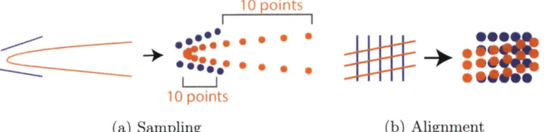
2-1 Drawbacks of Chamfer distance. In (a), sampling from Bdzier curve
B (blue) by uniformly sampling in parameter space yields
dispropor-tionately many points at the high-curvature area, resulting in a low Chamfer distance to the segments of A (orange) despite geometric dissimilarity. In (b), two sets of nearly-orthogonal line segments have near-zero Chamfer distance despite misaligned normals. . . . . 23
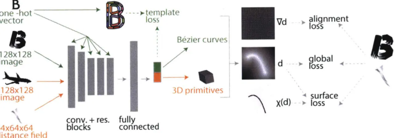
2-2 An overview of our pipelines-font vectorization (green) and volumetric primitive prediction (orange). . . . . 26 2-3 Vectorization of various glyphs. For each we show the raster input (top
left, gray) along with the vectorization (colored curves) superimposed. When the input has simple structure (a), we recover an accurate vec-torization. For fonts with decorative details (b), our method places template curves to capture overall structure. Results are taken from the test dataset. . . . . 28
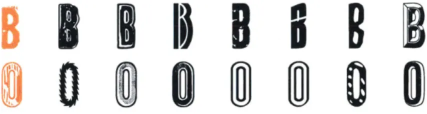
2-4 Glyphs with corresponding predicted curves rendered with predicted stroke thickness. The network thickens curves of to account for stylistic
details.. .. . . . . . . .. .. . . . . 29
2-5 Font glyph templates. These determine the connectivity and initialize the placement of the predicted curves. . . . . 30 2-6 Nearest neighbors for a glyph in curve space, sorted by proximity. The
2-7 Interpolating between fonts in curve space. The start and end are shown in orange and blue, resp., and nearest-neighbor glyphs to linear interpolants are shown in order. . . . . 32 2-8 Number of examples per quantized loss value. We visualize the input
and predicted curves for several outliers. . . . . 32 2-9 User-guided font exploration. At each edit, the nearest-neighbor glyph
is displayed on the bottom. This lets the user explore the dataset through geometric refinements. . . . . 33
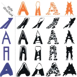
2-10 Mixing of style (columns) and structure (rows) of the A glyph from dif-ferent fonts. We deform each starting glyph (orange) into the structure of each target glyph (blue). . . . . 33
2-11 Vectorization of GAN-generated fonts from [41. . . . . 34 2-12 Comparisons to missing terms and Chamfer. . . . . 36 2-13 Cuboid shape abstractions on test set inputs. In (a) and (b), we show
ShapeNet chairs and airplanes. In (c), we show Shape COSEG chair segmentation. We show each input model (left) next to the cuboid representation (right). . . . . 38
2-14 Single view reconstruction using different primitives and boolean oper-ations. . . . . 38 3-1 Given a bitmap sketch of a man-made shape, our method automatically
infers a complete parametric 3D model, ready to be edited, rendered, or converted to a mesh. Compared to conventional methods, our resolution-independent geometry representation allows us to faithfully reconstruct sharp features (wing and tail edges) as well as smooth regions. Results are shown on sketches from a test dataset. Sketches in this figure are upsampled from the actual images used as input to our method. . . . 40
3-2 Our data generation and augmentation pipeline. Starting with a 3D model (a), we use Autodesk Maya to generate its contours (b), which we vectorize using the method of [12] and stochastically modify (c). We then use the pencil drawing generation model of [84] to generate the
final im age (d). . . . . 44 3-3 Our geometry representation is composed of Coons patches (a) that are
organized into a deformable template (b). We have designed a separate template per category of shapes: guitars (b), planes, bathtubs, and
knives (c). . . . . 47
3-4 Intersection scores predicted by the self-intersection MLP evaluated on 50 patches linearly interpolated between a flat patch and a patch with several self-intersections. The score increases as the patch becomes "more self-intersecting." Six out of the 50 patches, including the initial
and final patches, are displayed. . . . . 51 3-5 Example patches misclassified by the self-intersection MLP. Two false
positives (incorrectly predicted to be self-intersecting) are shown in green, and two false negatives are shown in orange. . . . . 51 3-6 An overview of our deep learning pipleine. We encode a sketch image
with a series of convolutions and residual blocks. Following a fully connected layer, we get back a series of parameters defining a collection of Coons patches. We then compute five loss values based on the predicted patches and the ground truth 3D model as well as a template. We optimize the overall loss using backpropagation. . . . . 52 3-7 Results on synthetic sketches taken from our test datasets for bathtubs,
guitars, and knives. . . . . 54
3-8 Results on real human-drawn sketches. The top two rows are sketches are drawn on pencil and paper and scanned while the bottom two rows are drawn on iPad. Each artist was shown the sample sample 3D models rendered from several viewpoints but was not provided with sample sketches or given instructions on how to draw the sketches. . . 55
3-9 For a human-drawn sketch (a), we perform an ablation study of our algorithm, training the network (b) without the self-intersection loss, (c) without pairwise intersection loss, (d) without normal loss, or using a simple template (e). We also study the effects of various data aug-mentation stages ( 3.2) by training the network: (f) only on contour
renders without any augmentation, (g) with the sketch filter, but no vector augmentation. In (h), we overlay (g, shown in brown) with the
final result (i). . . . . . . . . 56
3-10 The template used for our main airplane model (left) and the simple airplane template used for the ablation study (right). The simple airplane template contains fewer patches than the main template, and, consequently, yields less expressive results. . . . . 56
3-11 Compared to the previous multi-view approaches, [27] (a) and
162]
(c), we (b and d) produce results of comparable quality with just a single sketch. Furthermore, unlike voxelization-based approaches [271 or smooth mesh-based [62], our models don't depend on resolution and can represent sharp and smooth regions explicitly. . . . . 573-12 Comparison to [27] for single-view reconstruction on inputs from our dataset. Their predictions (graciously generated by the authors) are in orange, and ours are in green. This experiment demonstrates that their method does not generalize to arbitrary single-view sketches. . . 58
3-13 3D reconstructions using AtlasNet [37] (b) and our method (c) given a single rendering as input (a). Compared to AtlasNet, we produce a result without topological defects (holes and overlaps). Additionally, each of our patch primitives is easily editable and has a low dimensional, interpretable parameterization. . . . . 58
A-1 Glyph nearest neighbors in curve space. . . . . 61
A-2 Interpolations between fonts in curve space. . . . . 61
A-4 Local loss (smoothed) over the first 4,000 iterations of training with and without global loss in the objective function. The global loss term
results in faster convergence. . . . . 62
A-5 Cuboid reconstructions of ShapeNet chairs. . . . . 63
A-6 Cuboid reconstructions of ShapeNet airplanes. . . . . 64
List of Tables
2.1 Comparison between subsets of our full loss as well as standard Chamfer distance. Average error is Chamfer distance (in pixels on a 128 x 128 image) between predicted curves and ground truth, with points sampled uniformly. This demonstrates advantages of our loss over Chamfer distance and shows how each loss term contributes to the results. . . 35
Chapter 1
Introduction
The creation, modification, and rendering of vector graphics and parametric shapes is a fundamental problem of interest to engineers, artists, animators, and designers. Such representations offer distinct advantages over other models. By expressing a shape as a collection of primitives, we are able to apply transformations easily, to identify correspondences, and to render at arbitrary resolution, all while having to store only a sparse representation.
It is often useful to generate a parametric model from data that does not directly correspond to the target geometry and contains imperfections or missing parts. This can be an artifact of noise, corruption, or human-generated input; often, an artist intends to create a precise geometric object but produces one that is "sketchy" and ambiguous. Hence, we turn to machine learning methods, which have shown success in inferring structure from noisy data.
Convolutional neural networks (CNNs) achieve state-of-the-art results in vision tasks such as image classification [52], segmentation [61], and image-to-image trans-lation [45]. CNNs, however, operate on raster representations. Grid structure is fundamentally built into convolution as a mechanism for information to travel between layers of a deep network. This structure is leveraged during training to optimize performance on a GPU. Recent deep learning pipelines that output vector shape primitives [95] have been significantly less successful than pipelines for analogous tasks on raster images or voxelized volumes.
In this thesis, we explore two different perspectives on CNN-based parametric shape prediction using. First, in Chapter 2, we look at the challenge of combining Eulerian and Lagrangian representations when applying deep learning to parametric geometry. CNNs process data in an Eulerian fashion in that they apply fixed operations to a dense grid of values; Eulerian shape representations like indicator functions come as values on a fixed grid. Parametric shapes, on the other hand, use sparse sets of parameters like control points to express geometry. In contrast to stationary Eulerian grid points, this Lagrangian representation moves with the shape. Navigating the transition from Eulerian to Lagrangian geometry is a key step in any learning pipeline for the problems above, a task we consider in detail.
We propose a deep learning framework for predicting parametric shapes, addressing the aforementioned issues. By analytically computing a distance field to the primitives at each training iteration, we formulate an Eulerian version of the Chamfer distance, a common metric for geometric similarity. Our metric can be computed efficiently and does not require sampling points from the predicted or target shapes. Beyond accelerating evaluation of existing loss functions, our distance field enables alternative loss functions that are sensitive to specific geometric qualities like alignment.
We apply our new framework in the 2D context to a diverse dataset of fonts. We train a network that takes in a raster image of a glyph and outputs a representation as a collection of B6zier curves. This maps glyphs onto a common set of parameters that can be traversed intuitively. We use this embedding for font exploration and retrieval, correspondence, and unsupervised interpolation.
We also show that our approach works in 3D. With surface primitives in place of curves, we perform volumetric abstraction on ShapeNet [16], inputting an image or a distance field and outputting parametric primitives that approximate the model. This output can be rendered at any resolution or converted to a mesh; it also can be used for segmentation.
In Chapter 3, we consider the task of sketch-based 3D modeling. Here the goal is to algorithmic interpret natural sketches to allow non-experts to quickly create expressive 3D content. Converting rough, incomplete 2D input into a clean, complete
3D shape is extremely ill-posed, requiring inference of missing parts and interpretation
of noisy sketch curves. To cope with these ambiguities, existing systems either tend to rely on hand-designed shape priors that are difficult to construct or produce output that often lacks resolution and sharp features necessary for high-quality 3D models.
To address these issues, we present a deep learning-based system to infer a complete man-made 3D shape from a single bitmap sketch. Given an expressive sketch of an object, our system infers a set of parametric surfaces that realize the drawing in 3D. The component surfaces, parameterized by their control points, allow for easy editing in conventional shape editing software or conversion to a manifold mesh.
Most sketch-based modeling algorithms target natural shapes like humans and animals [29, 10, 44], which are naturally smooth. To aid shape reconstruction, these systems promote smoothness of the reconstructed shape; representations like general-ized cylinders are chosen to optimize in the space of smooth surfaces [29, 10]. This principle, however, does not apply to the focus of our work: man-made shapes. These objects, like planes or espresso machines, are only piecewise smooth and hence do not satisfy the assumptions of many sketch-based modeling systems.
In industrial design, man-made shapes are typically modeled using collections of smooth parametric patches, such as NURBS surfaces, with patch boundaries forming the sharp features. To learn such shapes effectively, we leverage this structure by using a special shape representation, a deformable parametric template [46]. This template is a manifold surface composed of patches, where each patch is parameterized by its control points. This representation enables us to control the smoothness of each patch while allowing the model to introduce sharp edges between patches where necessary. Compared to traditional representations, deformable parametric templates have numerous benefits for our task. They are intuitive to edit with conventional software, are resolution-independent, and can be meshed to arbitrary accuracy. Furthermore, since typically only boundary control points are needed, our surface representation has relatively few parameters to learn and store. Finally, this structure admits closed-form expressions for normals and other geometric features, which can be used to construct loss functions that improve reconstruction quality ( 3.3.2).
The core of our system is a CNN-based architecture to infer the coordinates of control points of a deformable template, given a bitmap sketch. A naive attempt to develop and train such network faces two major challenges: 1) lack of realistic sketch data and 2) the difficulty of detecting self-intersecting surfaces. To address these two issues, we 1) introduce a synthetic sketch augmentation pipeline that uses insights from the artistic literature to simulate possible variations observed in natural drawings and 2) train two networks to predict shape self-intersections given shape parameters, using these networks as additional loss terms in the optimization for sketch-based modeling to regularize our patches.
Chapter 2
Shape Predictions using Distance
Fields
2.1
Related Work
Font exploration and manipulation. Designing or even finding a font can be tedious using generic vector graphics tools. Certain geometric features distinguish letters from one another across fonts, while others distinguish fonts from one another. Due to these difficulties and the presence of large font datasets, font exploration, design, and retrieval have emerged as challenging problems in graphics and learning. Previous exploration methods categorize and organize fonts via crowdsourced attributes [691 or embed fonts on a manifold using purely geometric features [15, 7]. Instead, we leverage deep vectorization to automatically generate a sparse represen-tation for each glyph. This enables exploration on the basis of general shape rather than fine detail.
Automatic font generation methods usually fall into two categories. Rule-based methods [89, 75] use engineered decomposition and reassembly of glyphs into parts. Deep learning approaches [4, 991 produce raster images, with limited resolution and potential for image-based artifacts, making them unfit for use as glyphs. We apply our method to edit existing fonts while retaining vector structure and demonstrate vectorization of glyphs from partial and noisy data, i.e., raster images from a generative
model.
Parametric shape collections. As the number of publicly-available 3D models grows, methods for organizing, classifying, and exploring models become crucial. Many approaches decompose models into modular parametric components, commonly relying on prespecified templates or labeled collections of specific parts 150, 82, 711. Such shape
collections prove useful in domain-specific applications in design and manufacturing
[79, 981. Our deep learning pipeline allows generation of parametric shapes to perform
these tasks. It works quickly on new inputs at test time and is generic, handling a variety of modalities without supervision and producing different output types.
Deep 3D reconstruction. Combining multiple viewpoints to reconstruct 3D
geom-etry is crucial in applications like robotics and autonomous driving [32, 80, 881. Even more challenging is inference of 3D structure from one input. Recent deep networks can produce point clouds or voxel occupancy grids given a single image [31, 22], but their output suffers from fixed resolution.
Learning signed distance fields defined on a voxel grid [26, 87] or directly 1721 allows high-resolution rendering but requires surface extraction; this representation is neither sparse nor modular. Liao et al. address the rendering issue by incorporating marching cubes into a differentiable pipeline,'but the lack of sparsity remains problematic, and predicted shapes are still on a voxel grid [56]
Parametric 3D shapes offer a sparse, non-voxelized solution. Methods for converting point clouds to geometric primitives achieve high-quality results but require supervision, either relying on existing data labelled with primitives [54, 68] or prescribed templates
[33]. Tulsiani et al. output cuboids but are limited in output type [951. Groueix
et al. output primitives at any resolution, but their primitives are not naturally parameterized or sparsely represented [38].
10 points I I 10 points (a) Sampling * 0 hILL-. (b) Alignment
Figure 2-1: Drawbacks of Chamfer distance. In (a), sampling from Bezier curve B
(blue) by uniformly sampling in parameter space yields disproportionately many points
at the high-curvature area, resulting in a low Chamfer distance to the segments of
A (orange) despite geometric dissimilarity. In (b), two sets of nearly-orthogonal line
segments have near-zero Chamfer distance despite misaligned normals.
2.2
Preliminaries
Let A, B
c
R' be two smooth (measurable) shapes. Let X and Y be two point sets
sampled uniformly from A and B. The directed Chamfer distance between X and Y is
(2.1)
Chdir (XY)
=
min d(x, y),
xX E
and the symmetric Chamfer distance is defined as
Ch(X, Y)
=
Chdir(X,Y)
+
Chdir (Y, X).(2.2)
It was proposed for computational applications in
[14]
and has been used as a loss
function assessing similarity of a learned shape to ground truth in deep learning
[95, 31, 60, 38].
We also define variational directed Chamfer distance
Ch r|(A, B)A =
hdir IJJA
inf ||X - Y112 dx,
yEB
with variational symmetric Chamfer distance Ch(A, B)Var defined analogously,
ex-tending (2.1) and (2.2) to smooth objects. We use this to relate our proposed loss to
Chamfer distance.
If points are sampled uniformly, under relatively weak assumptions about A and
(2.3)
00
040
B, Ch(X, Y)
-+0 iff A
=
B, as the sizes of the sampled point sets grow. Thus, it is
a reasonable shape matching metric. Chamfer distance, however, has fundamental
drawbacks:
" It is highly dependent on the sampled points and sensitive to non-uniform sampling,
as in Figure 2-la.
* It is slow to compute. For each x sampled from A, it is necessary to find the closest
y sampled from B, a quadratic-time operation when implemented naYvely. Efficient
structures like k-d trees are not well-suited to GPUs.
" It is agnostic to normal alignment. As in Figure 2-1b, the Chamfer distance between
a dense set of vertical lines and a dense set of horizontal lines approaches zero.
Our method does not suffer from these disadvantages.
2.3
Method
Beyond architectures for particular tasks, we introduce a framework for formulating
loss functions suitable for learning placement of parametric shapes in 2D and 3D;
our formulation not only encapsulates Chamfer distance-and suggests a means of
accelerating its computation-but also leads to stronger loss functions that improve
performance on a variety of tasks. We start by defining a general loss on distance
fields and propose three specific losses.
2.3.1
General Distance Field Loss
Given A, B
C R,let dA,
dB: R
n -R+ measure distance from each point in Rn
toA or B, respectively,
dA(x) :=infYEA fX
- Y112.In our experiments, n E
{2,
3}. Let
S C R
nbe a bounded set with A, B C S. We define the general distance field loss as
I2I [A, B]
=j
SI'A,B(x)dV(x),
(2.4)
for some measure of discrepancy T. Note that we represent A and B only by their
respective distance functions, and the loss is computed over S.
Let D E RP be a collection of parameters defining a shape. For instance, a parametric shape may consist of Bezier curves, in which case 4 contains a list of control points. Let d4 : R"n -+ R+ be the distance to the shape defined by 4. Given a
target object T with distance function dT, we formulate fitting a parametric shape to
approximate T w.r.t. T as minimizing
h (() = L
2[4,
T]. (2.5)For optimal shape parameters, <D := arg min,
fp(D).
We propose three discrepancy measures, providing loss functions that capture different geometric features.2.3.2
Surface Loss
We define surface discrepancy to be
'sJ"L
(x)=6{kerdA}(x)dB(x)+6{ker
dB}(x)dA(x)(2.6)
where 6{X} is the Dirac delta defined uniformly on X, and ker
f
denotes the zerolevel-set of
f.
Ipsurf is only nonzero where the shapes do not match, making it sensitive to fine details in the matching:Proposition 1 The symmetric variational Chamfer distance between A, B C Rn
equals the corresponding surface loss between, i.e., Ch"r (A, B) = L .
A,B
Unlike the Chamfer distance, the discrete version of our surface loss can be approx-imated efficiently on GPU without sampling points from either the parametric or target shape.
2.3.3
Global Loss
We define global discrepancy to be
B
one -hot ).-- template
vector loss Bezier curve 128x128
Ee
image128x128
I I3D
primitives
imageflcony. + res. fully
64x64x64 blocks connected distance field I, Vd alignment d + c bal Xd surface X(d) - loss
Figure 2-2: An overview of our pipelines-font vectorization (green) and volumetric
primitive prediction (orange).
Minimizing L.,glob is equivalent to minimizing the
L2distance between
dAand
dB-A,B
fFglob
(I)
increases quadratically in distance between the shape defined
by (D and the
target shape. Thus, minimizing
fpglob
encourages global alignment, quickly placingthe parametric primitives close to the target and accelerating convergence.
2.3.4
Normal Alignment Loss
We define normal alignment discrepancy to be
qf"(i ) = |V
d2(x)
-V
d
2(x)Ij.(2.8)
Minimizing fjaiign aligns normals of the predicted primitives to those of the target. Following Figure 2-1b, if A contains dense vertical lines and B contains horizontal
lines,
augnis large while Ch(A, B)
~0.
A,B
2.3.5
Final Loss Function
The general distance field loss and the specific discrepancy measures proposed thus far are differentiable w.r.t the shape parameters 4, as long as the distance function d. is differentible w.r.t. 4. Thus, they are well-suited to be optimized by a deep network
B
that predicts parametric shapes. To discretize, we simply redefine (2.4) to be
L
4[A,
B]
=E
'A,B(X),(2.9)
xEG
where G is a 2D or 3D grid. Thus, we minimize a weighted sum of
fp(oID)
across the
T defined in 2.3:
F = pglob + asur4 surf - ozalignalig".
(2.10)
We use asurf =
1
and oa"ig - 0.001 across experiments. In 3D experiments, we decaythe global loss term exponentially by a factor 0.5 every 500 iterations.
2.3.6
Network architecture
The network takes a 128x 128 image or a 64x64x64 distance field as input and outputs
a parametric shape. We use the same architecture for 2D and 3D, following advances
in network architecture design. Let c5s2-64 be a convolutional layer with 64 filters
of 5 x 5 evaluated at stride 2, Rx7 be 7 residual blocks [42, 41] of size 3 x 3 (keeping
filter count constant), and f c-512 be a fully-connected layer. To increase receptive
field without dramatically increasing parameter count, we also use dilated convolution
[113, 17] in residual blocks. We use ELU [23] after all linear layers except the last. We
use LayerNorm [5] after each conv and residual layer, except the first. Our encoder
architecture is: c5sl-32, c3s2-64, c3sl-64, c3s2-128, c3sl-128, c3sl-128, c3s2-256,
Rx7, c3s2-256, Rxl, c3s2-256, Rxl, f c-512, f c-N, where N is the dimension of our target parameterization. Our pipeline is illustrated in Figure 2-2. We train each network on a single Tesla
K80 GPU, using Adam [51]
with learning rate 104 andbatch size 16.
2.4
2D: Font Exploration and Manipulation
We demonstrate our method in 2D for font glyph vectorization. Given a raster image
of a glyph, our network outputs control points that form a collection of quadratic
AABB
CCD
EE
EE
FF&G
HHII
IJ
FP
G
+
JJ
KLMNN00
KK
LI
M
RRO
(a) Plain font glyphs (b) Decorative font glyphs
Figure 2-3: Vectorization of various glyphs. For each we show the raster input (top left, gray) along with the vectorization (colored curves) superimposed. When the input has simple structure (a), we recover an accurate vectorization. For fonts with decorative details (b), our method places template curves to capture overall structure.
Results are taken from the test dataset.
B6zier curves approximating its outline. When used on a glyph of a simple font (non-decorative, e.g., sans-serif), our method recovers nearly the exact original vector representation. From a decorative glyph with fine-grained detail, however, we recover a good approximation of the glyph's shape using relatively few B6zier primitives and a consistent structure. This process can be interpreted as projection onto a common sparse latent space of control points.
We first describe our choice of primitives as well as the computation of their distance fields. We introduce a template-based approach to allow our network to better handle multimodal data (different letters) and test several applications.
2.4.1
Approach
Primitives
We wish to use a 2D parametric shape primitive that is sparse and expressive and admits an analytic distance field. Our choice satisfying these requirements is the
quadratic Bezier curve, which we will refer to as curve, parameterized by control points
a, b, c E R2 and defined by B(t) = (1-t) 2a+2(1-t)tb+t2c, for 0 < t < 1. We represent 2D shapes as the union of n curves parameterized by <P = {ai, b,, ci, ... , an, bn, cn},
where ai, ci, bi E R2
0
N-N
N
Figure 2-4: Glyphs with corresponding predicted curves rendered with predicted stroke
thickness. The network thickens curves of to account for stylistic details.
the t G
R
such that B(i) is the closest point on the curve to p satisfies the following:
(B, B)i
3+ 3(A, B)i2 + (2(A, A) + (B, a
-
p))(
+ (A, a - p) = 0,
where A = b - a and B = c - 2b+ a.
Thus, evaluating the distance to a single curve d(p, Bj)
=11p
-Bi()
112requires
finding the roots of a cubic [76], which we can do analytically in constant time. To
compute distance to the union of the curves, we take a minimum:
d4,(p) = mindBi(p). (2.12)
i=1
In addition to the control points, we predict a stroke thickness parameter for each
curve. We use this parameter when computing the loss by "lifting" the predicted
distance field and, consequently, thickening the curve-if a curve B has stroke thickness
s, we set ds (p) = min(dB(p)
-s,
0).While we do not visualize stroke thickness in
our experiments, this approach allows the network to thicken curves to better match
fine-grained decorative details (Figure 2-4). This thickening is a simple and natural
operation in our distance field representation; note that sampling-based methods do
not provide a natural way to "thicken" the surfaces.
Templates
Our training procedure is unsupervised, as we do not have ground truth curve
annotations. To better handle the multimodal nature of our data without a separate
network for each letter, we label each training example with its letter, passed as
additional input to our network. This allows us to condition based on input class
ABCDEFGH
JKLM
NOPQRSTUVWXYZ
0
(a) Letter templates (b) Simple templates
Figure 2-5: Font glyph templates. These determine the connectivity and initialize the placement of the predicted curves.
layer (after replicating to the appropriate spatial dimensions), a common technique
for conditioning [116].
We choose a "standard" Bezier curve representation for each letter, which captures that letter's distinctive geometric and topological features, by designing 26 templates from a shared set of control points output by our network. A template of class
E
{A, ... , Z} is a collection of points Te = {Pi, . . . , pn} C R2 with correspondingconnectivity determining how points in T are used to define curves. Since we predict
glyph boundaries, our final curves form closed loops, allowing us to reuse endpoints.
For extracting glyph boundaries from uppercase English letters, there are three
connectivity types-one loop (e.g., C), two loops (e.g., A), and three loops (B). We
design templates such that the first loop has 15 curves and the other loops have 4 curves each. Our templates are shown in Figure 2-5a. We will show that while letter templates (a) are better able to specialize to the boundaries of each glyph, we still achieve good results for most letters with the simple templates (b), which also allow for establishing cross-glyph correspondences.
We use predefined templates together with our labeling of each training example for two purposes. First, connectivity is used to compute curve control points from the network output. Second, they provide a template loss
template(c,
)
= atemplateW(t/s) Tc - ht(x) 11,(2.13)
where s
E
Z+, 7 E (0, 1), and t is the current iteration. This serves to initialize thenetwork output, such that a training example of class f initially maps to template letter
f; as the loss decays during training, it acts as a regularizer. We choose atemplate = 1,
S
0
0
0
0
Figure 2-6: Nearest neighbors for a glyph in curve space, sorted by proximity. The
query glyph is in orange.
2.4.2
Experiments
We train our network on the 26 uppercase English letters extracted from nearly 10,000
fonts. The input is a raster image of a letter, and the target distance field to the
boundary of the original vector representation is precomputed.
Vectorization
For any font glyph, our method generates a sparse vector representation, which
robustly and accurately describes the glyph's structure while ignoring decorative and
noisy details. For simple fonts comprised of few strokes, our representation is a nearly
perfect vectorization, as in Figure 2-3a.
For glyphs from decorative fonts, our method produces a meaningful representation.
In such cases, a true vectorization would contain many curves with a large number of
connected components. Our network places the sparse curve template to best capture
the glyph's structure, as in Figure 2-3b.
Our method preserves semantic correspondences in our templates. The same curve
is consistently used for the boundary of, e.g., the top of an L These correspondences
persist
across
letters for both letter templates and simple templates-see for example
the E and F glyphs in Figure 2-3a and 2-3b and "simple templates" in Figure 2-12.
We demonstrate robustness in Figure 2-8 by quantizing our loss values and
visual-izing the number of examples for each value. Outliers corresponding to higher losses
are generally caused by noisy data-they are either not uppercase English letters or
have fundamentally uncommon structure.
EL
F
CC
EAEEAAVC
C
AA-EE E
Figure 2-7: Interpolating
in orange and blue, resp.,
in order.
101 -104 -101 102 101 100between fonts in curve space. The start and end are shown
and nearest-neighbor glyphs to linear interpolants are shown
0
Figure 2-8: Number
predicted curves for
4
loss value (xle-3)
6 8
of examples per quantized loss value. We visualize the input and
several outliers.
Retrieval and Exploration
Our sparse representation can be used to explore the space of glyphs, useful for artists
and designers. By treating the control points as a metric space, we can perform
nearest-neighbor lookups to retrieve fonts using Euclidean distance.
In Figure 2-6, for each query, we compute its curve representation and retrieve
seven nearest neighbors in curve space. Because our representation uses geometric
structure, we find fonts that are similar structurally, despite decorative and stylistic
differences.
We can also consider a path in curve space starting at the curves for one glyph
and ending at those for another. By sampling nearest neighbors along this trajectory,
we interpolate between glyphs. As in Figure 2-7, this produces meaningful collections
of fonts for the same letter and reasonable results when the start and end glyphs are
different letters. Additional results are available A.
r.
AAAA
AAAA
Figure 2-9: User-guided font exploration. At each edit, the nearest-neighbor glyph is
displayed on the bottom. This lets the user explore the dataset through geometric
refinements.
A
A
AAAA
AA
A
Figure 2-10: Mixing of style (columns) and structure (rows) of the A glyph from
different fonts. We deform each starting glyph (orange) into the structure of each
target glyph (blue).
Nearest-neighbor lookups in curve space also can help find a font matching desired
geometric characteristics. A possible workflow is in Figure 2-9-through incremental
refinements of the curves the user can quickly find a font.
Style and Structure Mixing
Our sparse curve representation describes geometric structure, ignoring stylistic
ele-ments (e.g., texture, decorative details). We leverage this to warp a glyph with desired
style to have a target structure of another glyph (Figure 2-10).
GAN-generated Ours
BB
HH
K~K
Figure 2-11:
Our (filled) Adobe lllustrator GAN-generated Ours
S S L
L
BB
P
HHIA P
Vectorization of)
JJ
GAN-generated
Our (filled) Adobe Illustrator
Uf
L
PP
J
fonts from
[4I.
We first generate the sparse curve representation for source and target glyphs. Since
our representation uses the same set of curves, we can estimate dense correspondences
and use them to warp original vectors of source glyph to conform to the shape of the
target. For each point p on the source, we find the closest point q on the its sparse
curve representation. We then compute the translation from q to the corresponding
point on the target glyph's sparse representation and apply this translation to p.
Repair
Our system introduces a strong prior on glyph shape, allowing us to robustly handle
noisy input. In [4], a generative adversarial network (GAN) generates new glyphs
based on samples. The outputs, however, are raster images, often with noise and
missing parts. Figure 2-11 shows how our method can simultaneously vectorize and
repair GAN-generated glyphs. Compared to a vectorization tool like Adobe Illustrator
Live Trace, we infer missing data to reasonably fit the template. This post-processing
step makes the glyphs from generative models usable starting points for font design.
Comparison and Ablation Study
We show a series of experiments that demonstrate the advantages of our loss over
standard Chamfer distance as well as the contributions of each term in our loss. We
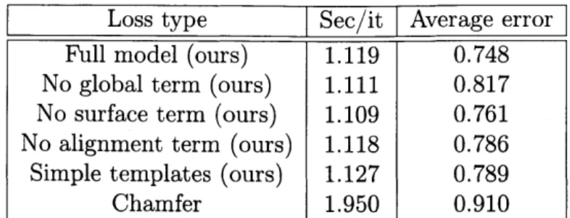
Loss type Sec/it Average error
Full model (ours)
1.119
0.748
No global term (ours) 1.111 0.817
No surface term (ours) 1.109 0.761
No alignment term (ours) 1.118 0.786
Simple templates (ours) 1.127 0.789
Chamfer
1.950
0.910
Table 2.1: Comparison between subsets of our full loss as well as standard Chamfer distance. Average error is Chamfer distance (in pixels on a 128 x 128 image) between predicted curves and ground truth, with points sampled uniformly. This demonstrates advantages of our loss over Chamfer distance and shows how each loss term contributes to the results.
demonstrate that while having 26 unique templates helps achieve better results, it is not crucial-we evaluate a network trained with three "simple templates" (Figure 2-5b), which capture the three topology classes of our data.
Table 2.1 shows seconds per iteration for our full distance field loss, our loss without each of its three terms and with simple templates, and Chamfer loss. Training using our loss is nearly twice as fast as Chamfer per iteration. Moreover, each of our loss terms adds <0.1 seconds. In these experiments, for training with the distance field function we use the same parameters as above, and for Chamfer loss, we use the same training procedure (hyperparameters, templates, batch size), sampling 5,000 points from the source and target geometry. We choose the highest possible value for which the sampled point pairwise distance matrix fits in GPU memory.
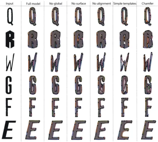
We also evaluate on 20 sans-serif fonts, computing Chamfer distance between our predicted curves and ground truth geometry, sampling uniformly (average error in Table 2.1). Uniform sampling is a computationally-expensive and non-differentiable procedure only for evaluation a posteriori-not suitable for training. While it does not correct all of the Chamfer distance's shortcomings, we use it as a baseline to evaluate quality. We limit to sans-serif fonts since we do not expect to faithfully recover local geometry. We see our full loss outperforms Chamfer loss, and all three loss terms are necessary. Here, all models are trained for 35,000 iterations. Figure 2-12 shows qualitative results on test set glyphs; see A for additional results.
Input Full model No global No surface No alignment Simple templates Chamfer
G
B
gil SI6
F
F F F F
EEEE'EEE
Figure 2-12: Comparisons to missing terms and Chamfer.
The global loss term strongly favors rough similarity between predicted and targeted
geometry, helping training converge more quickly (see Figure A-4).
2.5
3D: Volumetric Primitive Prediction
We reconstruct 3D surfaces out of various primitives, which allow our model to be
expressive, sparse, and abstract.
2.5.1
Approach
Our first primitive is a cuboid, parameterized by
{b,
t, r}, where b
=(w, h, d), t E R
3and r E
4a quaternion, i.e., an origin-centered (hollow) rectangular prism with
dimensions 2b to which we apply rotation r and then translation t.
p=
r-
1(p
-
t)r using the Hamilton product. Then, the signed distance between p and
C is
d(p, C)
=I max(d, 0)1|2 + min(max(d2, dy, dz), 0),
(2.14)
where d
= (|p'1,
|p'|, \p'l)
-b and v, vy, vz denote the x-, y-, and z-coordinates,
respectively, of vector v.
Our second primitive is a sphere, parameterized by its center c E R
3and radius r
E
R.
We compute signed distance to the sphere S via the expression d(p, S)
=||p
- c112 - r.Since these distances are signed, we can compute the distance to the union of
n primitives as in the 2D case, by taking a minimum over the individual primitive
distances. Similarly, we can perform other boolean operations, e.g., difference. The
result is, again, a signed distance function, and so we take its absolute value before
computing losses.
2.5.2
Experiments
We train on the airplane and chair categories of ShapeNet [16 using distance fields
from [26]. The input is a distance field. Hence, our method is self-supervised: The
distance field is the only information needed to compute the loss. Additional results
are available in A.
Surface abstraction. Figure 2-13 shows results of training shape-specific networks
to build abstractions over chairs and airplanes from 64 x 64 x 64 distance fields. Each
network outputs 16 cuboids. We discard small cuboids with high overlap as in
[95].
The resulting abstractions capture high-level structures of the input.
Segmentation.
Because we place cuboids in a consistent way, we can use them for
segmentation. Following
[95],
we demonstrate on the COSEG chair dataset. We first
label each cuboid predicted by our network (trained on ShapeNet chairs) with one
of the three segmentation classes in COSEG (seat, back, legs). Then, we generate a
cuboid decomposition of each chair mesh in the dataset and segment by labelling each
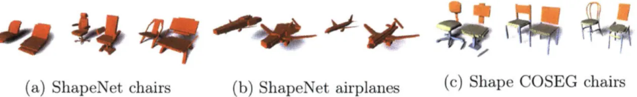
(a) ShapeNet chairs (b) ShapeNet airplanes (c) Shape COSEG chairs Figure 2-13: Cuboid shape abstractions on test set inputs. In (a) and (b), we show ShapeNet chairs and airplanes. In (c), we show Shape COSEG chair segmentation. We show each input model (left) next to the cuboid representation (right).
Figure 2-14: Single view reconstruction using different primitives and boolean
opera-tions.
face according to its nearest cuboid (Figure 2-13c). We achieve a mean accuracy of 94.6%, exceeding the 89.0% accuracy reported by
195].
Single view reconstruction. In Figure 2-14, we show results of a network that
takes as input a ShapeNet model rendering and outputs parameters for the union of four cuboids minus the union of four spheres. We see that for inputs that align well with this template, the network produces good results. It is not straightforward to
achieve unsupervised CSG-style predictions using sampling-based Chamfer distance loss.
Chapter 3
Sketch-Based Modeling of Man-Made
Shapes
3.1
Related Work
Our research leverages recent progress in deep learning to address long-standing
problems in sketch-based modeling. To give a rough idea of the landscape of available
methods, we briefly summarize related work in sketch-based modeling and deep
learning.
3.1.1
Sketch-based 3D shape modeling
Reconstructing 3D geometry from sketches has a long history in the computer graphics
literature. A complete survey of sketch-based modeling is beyond the scope of this
paper; an interested reader may refer to the recent paper by
[27]
or surveys by [28]
and [70]. Here, we mention the work most relevant to our approach.
Many sketch-based 3D shape modeling systems are incremental, i.e., they allow
users to model shapes by progressively adding new strokes, updating the 3D shape
after each action. Such systems may be designed as single-view interfaces, where the
user is often required to manually annotate each stroke [20, 36, 83, 18], or they may
allow strokes to be added to multiple views [44, 90, 67]. These systems can cope with
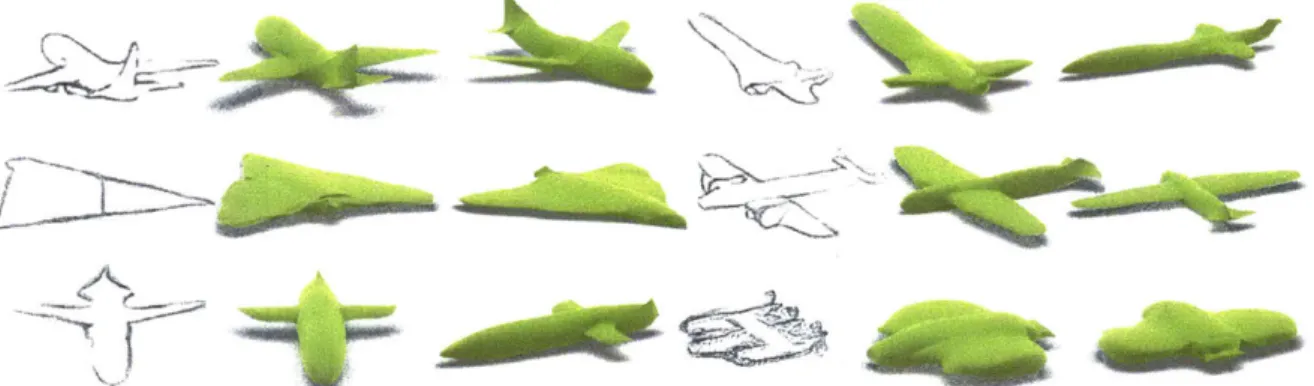
Figure 3-1: Given a bitmap sketch of a man-made shape, our method automatically
infers a complete parametric 3D model, ready to be edited, rendered, or converted to
a mesh. Compared to conventional methods, our resolution-independent geometry
representation allows us to faithfully reconstruct sharp features (wing and tail edges)
as well as smooth regions. Results are shown on sketches from a test dataset. Sketches
in this figure are upsampled from the actual images used as input to our method.
considerable geometric complexity, but their dependence on the ordering of the strokes
forces artists to deviate from standard approaches to sketching. In contrast, we aim
to interpret complete sketches, eliminating training for artists to use our system and
enabling 3D reconstruction of legacy sketches.
[1091
present a single-view 3D curve
network reconstruction system for man-made shapes that can produce impressive
sharp results. Yet, they process specialized design sketches, consisting of cross-sections,
output only a curve network without the surface, and rely on user annotations. Our
system produces complete 3D shapes from natural sketches with no extra annotation.
A variety of systems interpret a complete 2D sketch with no extra information. This
species of input is extremely ambiguous thanks to hidden surfaces and noisy sketch
curves, and hence reconstruction algorithms rely on strong 3D shape priors. These
priors are typically manually created by experts. For example, priors for humanoid
characters, animals, or natural shapes promote smooth, round, and symmetrical shapes
[10, 44, 29], while garments are typically regularized to be (piecewise-)developable
[55, 53, 47, 117, 78,
971,
and man-made shapes are often approximated as combinations
of geometric primitives [81] or as unions of nearly-flat faces
[1111.
Our work focuses on
man-made shapes, which have characteristic sharp edges and are only piecewise smooth
rather than developable. We use a deformable patch template to promote shapes
with
this structure ( 3.3.1). Moreover, introducing specific expert-designed priors can be challenging: Man-made shapes are varied, diverse, and complex (Fig. 3-1,3-7,3-8). Instead, we automatically learn a separate, perhaps stronger, shape prior for each category of shapes from data. This stronger category-specific prior allows us to process ambiguous and complex sketches.
The vast majority of sketch-based modeling interfaces process vector input, which consists of a set of clean curves [10, 13, 29, 53, 55, 47, 109]. This approach is acceptable for tablet-based input, but it again may force the users to deviate from their preferred drawing media. Paper-and-pencil sketches still remain one of the most preferred means of capturing a shape.. While those can be vectorized and cleaned up by modern methods [12, 84], preprocessing can introduce unnecessary distortions and errors into the drawing, leading to suboptimal reconstruction. In contrast, our system processes
bitmap sketches, scanned or digital.
3.1.2
Deep learning for shape reconstruction
Learning to reconstruct 3D geometry from various input modalities recently has enjoyed significant research interest. Typical forms of input are images [34, 105, 27,
110, 100, 21, 40] and point clouds [104, 37, 73]. When designing network for this task,
two important questions affect the architecture: the loss function and the geometric representation.
Loss functions. One promising and popular direction employs a differentiable renderer and measures 2D image loss between a rendering of the inferred 3D model and the input image, often called 2D-3D consistency or silhouette loss [49, 106, 110,
77, 105, 96, 93]. A notable example is the work by [105], which learns a mapping
from a photograph to a three-piece output of normal map, depth map, and silhouette, as well as the mapping from this output to a voxelization. They use a differentiable renderer and measure inconsistencies in 2D. 2D losses are powerful in typical computer vision environments. Hand-drawn sketches, however, cannot be interpreted as perfect projections of 3D objects: They are imprecise and often inconsistent [13]. Another
approach uses 3D loss functions, measuring discrepancies between the predicted and target 3D shapes directly, often via Chamfer or a regularized Wasserstein distance [104, 59, 63, 37, 73, 34], or-in the case of highly-structured representations such as voxel grids-sometimes cross-entropy [401. We build on this work, adapting the Chamfer distance to our novel geometric representation and extending the loss function with new regularizers ( 3.3.2).
Shape representation. As noted by
173],
geometric representations in deep learning broadly can be divided into three classes: voxel-based representations, point-based representations, and mesh-based representations.The most popular approach is to use voxels, directly reusing successful methods for
2D images [27, 105, 110, 100, 21, 115, 114, 108, 102, 931. The main limitation of
voxel-based methods is low resolution due to memory limitations. Octree-voxel-based approaches mitigate this problem [40, 101], learning shapes at up to 5123 resolution, but even this density is insufficient to produce visually convincing surfaces. Furthermore, voxelized approaches cannot directly represent sharp features, which are key for man-made shapes.
Point-based approaches represent 3D geometry as a point cloud [63, 30, 62, 91, 112], sidestepping the memory issues. Those representations, however, do not capture connectivity. Hence, they cannot guarantee production of manifold surfaces.
Some recent methods explore the possibility of reconstructing mesh-based repre-sentations [6, 8, 57, 48, 103], representing shapes using deformable meshes. We take inspiration from this approach to reconstruct a surface by deforming a template, but our deformable parametric template representation allows us to more easily enforce piecewise smoothness and test for self-intersections ( 3.3.2). These tasks are difficult to perform on meshes in a differentiable manner. Other mesh-based methods either use a precomputed parameterization to a domain on which it is straightforward to apply CNN-based architectures [64, 85, 39] or learn a parameterization directly [37, 9]. Even though these methods are not specifically designed for sketch-based modeling, for completeness, we compare our results to one of the more popular methods, AtlasNet