ÉCOLE DE TECHNOLOGIE SUPÉRIEURE UNIVERSITÉ DU QUÉBEC
THESIS PRESENTED TO
ÉCOLE DE TECHNOLOGIE SUPÉRIEURE
IN PARTIAL FULFILLMENT OF THE REQUIREMENTS FOR THE DEGREE OF DOCTOR OF PHILOSOPHY
Ph. D.
BY Abdalla BALA
IMPACT ANALYSIS OF A MULTIPLE IMPUTATION TECHNIQUE FOR HANDLING MISSING VALUE IN THE ISBSG REPOSITORY OF SOFTWARE PROJECTS
MONTREAL, OCTOBER 17 2013
This Creative Commons licence allows readers to download this work and share it with others as long as the author is credited. The content of this work can’t be modified in any way or used commercially.
THIS THESIS HAS BEEN EVALUATED BY THE FOLLOWING BOARD OF EXAMINERS
Mr. Alain Abran, Thesis Supervisor
Software Engineering and Information Technology Department at École de technologie supérieure
Mr. Ambrish Chandra, President of the Board of Examiners
Department of Electrical Engineering at École de technologie supérieure
Mr. Alain April, Member of the jury
Software Engineering and Information Technology Department at École de technologie supérieure
Mr. Chadi el Zammar, External Evaluator Kronos (Canada)
THIS THESIS WAS PRENSENTED AND DEFENDED
IN THE PRESENCE OF A BOARD OF EXAMINERS AND PUBLIC ON OCTOBER 16, 2013
ACKNOWLEDGMENTS
I would like to express my thanks and gratitude to Allah, the Most Beneficent, the Most Merciful whom granted me the ability and willing to start and complete this research.
First, I would like to express my utmost thanks to Dr. Alain Abran, my thesis supervisor, for his motivation, guidance, time and support. His advice continuously opened new opportunities to improve the outcomes of this research; without his patient support this research would have never been executed.
Thanks to the members of my board of examiners for their time and effort to review this thesis and to provide me with their feedback.
I am deeply and forever indebted to my parents Mr. Ali Bala and Mdm. Nagmia for their love, support and encouragement throughout my entire life. I am also very grateful to all my brothers Amer Bala, Mustafa Bala, Nuri Bala and to all my sisters for instilling in me confidence and a drive for pursuing my PhD.
I also would like to thank to those who have helped me and encouraged me at all time during my study: they are Adel Alraghi, Walid Bala, and special thanks to all my colleagues and my friends.
IMPACT ANALYSIS OF A MULTIPLE IMPUTATION TECHNIQUE FOR HANDLING MISSING VALUE IN THE ISBSG REPOSITORY OF SOFTWARE
PROJECTS Abdalla BALA
RÉSUMÉ
Jusqu'au début des années 2000, la plupart des études empiriques pour construire des modèles d'estimation de projets logiciels ont été effectuées avec des échantillons de taille très faible (moins de 20 projets), tandis que seules quelques études ont utilisé des échantillons de plus grande taille (entre 60 à 90 projets). Avec la mise en place d’un répertoire de projets logiciels par l'International Software Benchmarking Standards Group - ISBSG - il existe désormais un plus grand ensemble de données disponibles pour construire des modèles d'estimation: la version 12 en 2013 du référentiel ISBSG contient plus de 6000 projets, ce qui constitue une base plus adéquate pour des études statistiques.
Toutefois, dans le référentiel ISBSG un grand nombre de valeurs sont manquantes pour un nombre important de variables, ce qui rend assez difficile son utilisation pour des projets de recherche.
Pour améliorer le développement de modèles d’estimation, le but de ce projet de recherche est de s'attaquer aux nouveaux problèmes d’accès à des plus grandes bases de données en génie logiciel en utilisant la technique d’imputation multiple pour tenir compte dans les analyses des données manquantes et des données aberrantes.
Mots-clés: technique multi-imputation, préparation des données ISBSG, identification des valeurs aberrantes, modèle d'estimation de l'effort de logiciel, critères d'évaluation.
IMPACT ANALYSIS OF A MULTIPLE IMPUTATION TECHNIQUE FOR HANDLING MISSING VALUE IN THE ISBSG REPOSITORY OF SOFTWARE
PROJECTS Abdalla BALA
ABSTRACT
Up until the early 2000’s, most of the empirical studies on the performance of estimation models for software projects have been carried out with fairly small samples (less than 20 projects) while only a few were based on larger samples (between 60 to 90 projects). With the set-up of the repository of software projects by the International Software Benchmarking Standards Group – ISBSG – there exists now a much larger data repository available for productivity analysis and for building estimation models: the 2013 release 12 of this ISBSG repository contains over 6,000 projects, thereby providing a sounder basis for statistical studies.
However, there is in the ISBSG repository a large number of missing values for a significant number of variables, making its uses rather challenging for research purposes.
This research aims to build a basis to improve the investigation of the ISBSG repository of software projects, in order to develop estimation models using different combinations of parameters for which there are distinct sub-samples without missing values. The goal of this research is to tackle the new problems in larger datasets in software engineering including missing values and outliers using the multiple imputation technique.
Keywords: multi-imputation technique, ISBSG data preparation, identification of outliers, analysis effort estimation model, evaluation criteria.
TABLE OF CONTENTS
Page
INTRODUCTION ...1
CHAPTER 1 LITERATURE REVIEW ...5
1.1 ISBSG data repository ...5
1.2 ISBSG data collection ...6
1.2.1 The ISBSG data collection process...7
1.2.2 Anonymity of the data collected ...9
1.2.3 Extract data from the ISBSG data repository ...9
1.3 Literature Review of ISBSG-based studies ...10
1.4 Methods for treating missing values ...15
1.4.1 Deletion Methods for treatment of missing values ...15
1.4.2 Imputation methods ...16
1.5 Techniques to deal with outliers ...21
1.6 Estimation Models ...23
1.6.1 Regression techniques ...23
1.6.2 Estimation models: evaluation criteria ...24
1.7 Summary ...25
CHAPTER 2 RESEARCH ISSUES AND RESEARCH OBJECTIVES ...29
2.1 Research issues ...29
2.2 Research motivation ...30
2.3 Research goal and objectives ...31
2.4 Research scope ...31
CHAPTER 3 RESEARCH METHODOLOGY ...33
3.1 Research methodology ...33
3.2 Detailed methodology for phase I: Collection and synthesis of lessons learned ...35
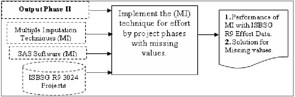
3.3 Detailed methodology for phase II: Data preparation and identification of outliers ...35
3.4 Detailed methodology for phase III: Multiple Imputation technique to deal with missing values ...36
3.5 Multiple imputation Overviews ...37
3.6 Detailed methodology for phase IV: Handling Missing values in effort estimation with and without Outliers...38
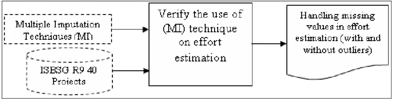
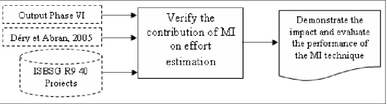
3.7 Detailed methodology for phase V: Verification the contribution of the MI technique on effort estimation ...39
CHAPTER 4 DATA PREPARATION AND IDENTIFICATION OF OUTLIERS...41
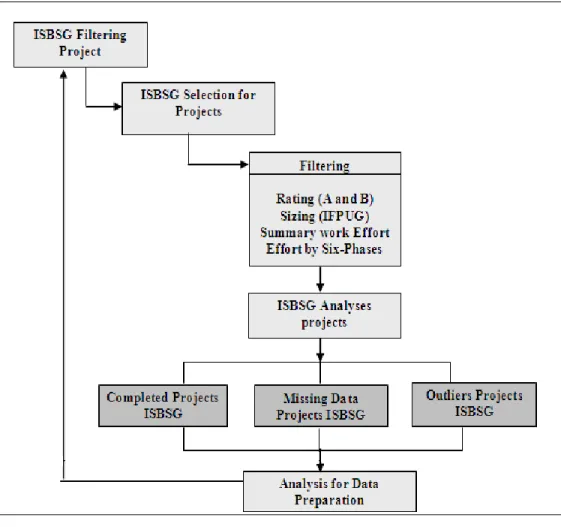
4.1 Data preparation ...41
4.2 Data preparation for ISBSG repository ...41
4.2.1 Data preparation effort by project phases ...41
4.4 Summary ...48
CHAPTER 5 MULTIPLE IMPUTATION TECHNIQUE TO DEAL WITH MISSING VALUES IN ISBSG REPOSITORY...49
5.1 Multiple imputation method in SAS soffware ...49
5.2 Implement the (MI) technique for effort by project phases with missing values ...51
5.2.1 Step 1 Creating the imputed data sets (Imputation) ...51
5.3 Step 2 analyzing the completed data sets ...63
5.3.1 Analysis strategy ...63
5.3.2 Implement effort estimation model (using the 62 imputed Implement values) ..64
5.3.3 Plan effort estimation models (built using the 3 imputed Plan values) ...66
5.4 Step 3 Combining the analysis results (combination of results) ...68
5.4.1 Strategy and statistical tests to be used ...68
5.4.2 The strategy for combining results ...69
5.4.3 Average parameter estimates for MI of the full imputed dataset (N= 106 and N=103) ...70
5.5 Summary ...74
CHAPTER 6 VERIFICATION OF THE CONTRIBUTION OF THE MI TECHNIQUE ON EFFORT ESTIMATION ...77
6.1 Introducation ...77
6.2 Strategy: creating artificially missing values from a complete dataset ...79
6.2.1 Strategy steps ...79
6.2.2 Impact on parameter estimates with outliers - N=41 and 21 projects with values deleted ...81
6.2.3 Impact on parameter estimates without outliers – N = 40 and 20 projects with values deleted ...82
6.2.4 Analysis of the variance of the estimates ...84
6.2.5 Additional investigation of effort estimation for N=20 projects with imputed values for the Effort Implement phase ...85
6.3 Sensitivity analysis of relative imputation of effort estimation for N=40 projects without outliers for the Effort Implement phase ...89
6.4 Comparing the estimation performance of MI with respect to a simpler imputation technique based on an average ...93
6.4.1 The (Déry et Abran, 2005) study ...93
6.4.2 Imputation based on an absolute average, %average, and MI with (absolute seeds and relative seeds Min & Max) ...97
6.4.3 Estimation model from Imputation based on an average...101
6.4.4 Comparisons between MI and imputation on averages (Absolute and relative seeds excluding outliers) ...103
6.5 Summary ...105
CONCLUSION ...109
LIST OF TABLES
Page
Table 1.1 Summary of ISBSG studies dealing with missing values and outliers ...14
Table 4.1 ISBSG data fields used ...44
Table 4.2 Number of projects with effort by phase in ISBSG R9 (Déry and Abran, 2005) ..45
Table 4.3 Descriptive Statistics for Grubbs' test on Total Effort (N=106) ...48
Table 4.4 Outlier analysis using Grubbs' test on Total Effort ...48
Table 4.5 Description of the 3 outliers deleted ...48
Table 5.1 Variance information for imputed values of Effort Plan and Effort Implement ....56
Table 5.2 Variance information for imputed values of Effort Plan and Effort Implement ....56
Table 5.3 Summary of imputed values for Effort Plan and Effort Implement ...56
Table 5.4 Average effort distribution per phase (1st Imputation) N=106 Projects ...57
Table 5.5 Average effort distribution per phase (2nd Imputation) N=106 Projects ...57
Table 5.6 Average effort distribution per phase (3rd Imputation) N=106 Projects ...58
Table 5.7 Average effort distribution per phase (4th Imputation) N=106 Projects ...58
Table 5.8 Average effort distribution per phase (5th Imputation) N=106 Projects ...58
Table 5.9 Comparison across the imputations with outliers (N=106 projects) ...59
Table 5.10 Average effort distribution for the 5 imputation (N=106 projects) ...59
Table 5.11 Average effort distribution per phase (1st Imputation) N=103 Projects ...60
Table 5.12 Average effort distribution per phase (2nd Imputation) N=103 Projects ...60
Table 5.13 Average effort distribution per phase (3rd Imputation) N=103 Projects ...61
Table 5.14 Average effort distribution per phase (4th Imputation) N=103 Projects ...61
Table 5.15 Average effort distribution per phase (5th Imputation) N=103 Projects ...61
Table 5.16 Comparison across the importations without outliers (N=103 projects) ...62
Table 5.17 Profiles of Average effort distribution for N=103 projects, excluding outliers ...62
Table 5.18 Regression analysis estimation model for Effort Implement based on the 5 imputed datasets (N=106 projects, with outliers) ...66
Table 5.19 Regression analysis estimation model for Effort Implement based on the 5 imputed datasets (N=103 projects, without outliers) ...66
Table 5.20 Regression analysis estimation model for Effort Plan based on the 5 imputed datasets (N=106 projects, with outliers) ...67 Table 5.21 Regression analysis estimation model for Effort Plan based on the 5 imputed
datasets (N=103 projects, without outliers) ...67 Table 5.22 Averages of parameter estimates of MI for Effort Implement (N=106) ...71 Table 5.23 Averages of parameter estimates of MI for Effort Implement (N=103
withoutoutliers) ...71 Table 5.24 Averages of parameter estimates of MI for Effort Plan (N=106) ...72 Table 5.25 Averages of parameter estimates of MI for Effort Plan (N=103 without 3
outliers) ...72 Table 5.26 Statistical significance of parameter estimates of Effort Plan ...73 Table 5.27 Statistical significance of parameter estimates of Effort Implement ...73 Table 6.1 Regression models for Effort Implement (N=41 projects, with outliers), before
and after missing values were removed for N=21 projects ...82 Table 6.2 Regression models for Effort Implement (N=40 projects, without an outlier),
before and after removing missing values for N = 20 projects ...83 Table 6.3 Verification results of the five imputed datasets for Effort Implement ...84 Table 6.4 Regression models for Effort Implement (N=20 projects, without an outlier) ...88 Table 6.5 Analysis of the EI estimation variance from estimation with imputed variance
and training estimation model ...88 Table 6.6 Multi-regression models for Effort Implement (from MI with relative seeds
for EI) ...92 Table 6.7 Contribution of relative imputation for N=40 projects with imputed values for
the Effort Implement phase ...92 Table 6.8 Average effort distribution by project phase including outliers (N=41 projects) ..96 Table 6.9 Average effort distribution by project phase excluding outliers (N=40
projects)...97 Table 6.10 Average effort distribution by project phase after imputations and by subsets-
Table 6.11 Average effort distribution by project phase after imputations and by subsets - excluding outliers (N=40 projects) ...100 Table 6.12 Average effort distribution after imputations – full dataset - including outliers
(N=41 projects) ...101 Table 6.13 Average effort distribution excluding outliers (N=40 projects) ...101 Table 6.14 Regression models for Effort Implement after imputations based on averages ..102 Table 6.15 Estimate variance of Effort Implement – Imputations based on averages ...103 Table 6.16 Comparison of models predictive performances ...104
LIST OF FIGURES
Page
Figure 1.1 ISBSG Data Collection Process ...8
Figure 3.1 General View of the Research Methodology ...34
Figure 3.2 Phase I: Collection and synthesis of lessons learned ...35
Figure 3.3 Phase 2: Identification of outliers in ISBSG Data set ...36
Figure 3.4 Phase III: Multiple Imputation Technique for missing values in ISBSG R9 ...36
Figure 3.5 Phase IV: Handling Missing values in effort estimation with and without Outliers ...38
Figure 3.6 Phase V: Verification the contribution of the MI technique on effort estimation ...39
Figure 4.1 ISBSG Data Preparation ...43
Figure 4.2 Data Preparation of ISBSG R9 Data set ...43
Figure 5.1 Multiple Imputation Processing ...50
Figure 5.2 Sample result of the multiple imputation method – step 1 ...54
Figure 5.3 Building the regression analysis estimation models ...64
Figure 6.1 Strategy for analyzing the predictive accuracy of an MI dataset using a subset with values deleted ...81
Figure 6.2 Modified strategy for the comparison with estimation models model trained with subset X of N= 20 projects ...87
Figure 6.3 Specific strategy for investigating MI based on relative EI seeds ...91
Figure 6.4 Sample of complete data N=40 projects ...94
Figure 6.5 Split of the 40 projects – withtout 1 outlier ...96
Figure 6.6 Imputation to subset Y based on absolute average EI of subset X ...98
LIST OF ABREVIATIONS
COSMIC Common Software Measurement International Consortium
EB Effort Build EI Effort Implement EP Effort Plan Eq Equation ES Effort Specify ET Effort Test
FiSMA Finnish Software Measurement Association
FP Functional Process
FPA Function Point Analysis
Hrs Hours
IEC International Electromechanical Commission IFPUC International Function Point Users Group
ISBSG International Software Benchmarking Standards Group ISO International Organization for Standardization
IT Information Technology
LMS Least Median Squares
MI Multiple Imputation
MMRE Mean Magnitude of Relative Error
MRE Magnitude of Relative Error
NESMA Netherlands Software Metrics users Association
PRED Prediction
PROC MIANALYSE Procedure Multiple Imputation Analysis PROC REG Procedure Regression Analysis PSBTI Plan, Specify, Build, Test, Implement
PSBT Plan, Specify, Build, Test
R9 Release 9
RE Relative Error
SBTI Specify, Build, Test, Implement
SD Standard Deviation
SE Standard Error
LIST OF SYMBOLS B Between: the imputation variance
N Number of projects
% Percentage
P Probability of obtaining a test statistic (p-value) P Parameter
T Total variance
U Within: the imputation variance
INTRODUCTION
Currently, there are many ways to develop software products and the scope of the effort estimation problem is much larger now than it was in the early days of software development in the 1960s when:
• most software was custom built, • projects had dedicated staff, and
• companies were usually paid on an effort basis (i.e. ‘cost plus’, or ‘time and materials’).
Underestimation of effort causes schedule delays, over-budgeting, poor software quality, dissatisfied customers, and overestimation of the effort leads to wasted software development resources. Thus, over the last three decades, a number of software effort estimation methods with different theoretical concepts have been developed (Jorgensen et Shepperd, 2007), some of which have combined previously existing effort estimation methods (Stephen et Martin, 2003); (Mittas et Angelis, 2008). To improve the accuracy of software effort estimation, many organizations collect software project data and use effort estimation models derived from these data sets (Shepperd et Schofield, 1997); (Jeffery, Ruhe et Wieczorek, 2000); (Lokan et Mendes, 2006); (Mendes et Lokan, 2008).
However, software engineering data sets typically contain outliers that can degrade the data quality. An outlier is defined as a data point that appears to be inconsistent with the rest of the data sets (Barnett et Lewis, 1995). If a software effort estimation model is built on a historical data set that includes outliers, then it is difficult to obtain meaningful effort estimates because the outliers can easily distort the model and degrade the estimation accuracy.
Missing values is another of the problems often faced in statistical analysis in general, and in multivariate analysis in particular (Everitt et Dunn, 2001). Furthermore, the proper handling of missing values becomes almost necessary when statistics are applied in a domain such as
software engineering, because the information being collected and analyzed is typically considered by submitters as commercially sensitive to the software organizations.
Software data quality is another crucial factor affecting the performance of software effort estimation; however, many studies on developing effort estimation models do not consider the data quality (Pendharkar, Subramanian et Rodger, 2005); (Sun-Jen et Nan-Hsing, 2006); (de Barcelos Tronto, da Silva et Sant'Anna, 2007); (Jianfeng, Shixian et Linyan, 2009).
While a number of researchers in the literature have used the ISBSG repository for research purposes, only a few have examined techniques to tackle : A) the data quality issue, B) the problem of outliers and C) the missing values in large multi-organizational repositories of software engineering data (Deng et MacDonell, 2008).
This thesis contains seven chapters. The current introduction outlines the organization of the thesis.
Chapter 1 presents the literature review of the ISBSG data repository, including the ISBSG data collection process. This chapter also presents a review of related work and establishes the theoretical framework for this research, followed by a focus on the modeling techniques to deal with missing values, as well techniques to deal with outliers. Finally this chapter presents the more frequently used quality criteria for the estimation techniques.
Chapter 2 presents a number of research issues identified from the analysis of the literature review on software effort estimation, as well the motivation of this research project. This chapter also presents the specific research goal and objectives, and the scope of this research.
Chapter 3 presents the general view and detailed view of the research methodology, as well as the methods selected to investigate the ISBSG dataset to deal with missing values and outliers before building estimation models.
Chapter 4 presents the detailed data preparation to explore the ISBSG data repository, followed by the two verification steps for the ISBSG dataset preparation, as well the selected variables used in this research. This chapter also presents the detailed effort by phase with the total project effort recorded in the ISBSG data repository. This chapter also presents the identification of outliers, and the use of the Grubbs test to deal with outliers and, as well the outliers behaviors in the ISBSG repository.
Chapter 5 investigates the use of the multiple imputation (MI) technique with the ISBSG repository for dealing with missing values. This chapter also presents the regression analysis trained with the imputed datasets (with and without outliers), as well the variance information of MI for estimation models (Effort plan and Effort Implement).
Chapter 6 presents the general strategy for measuring the predictive accuracy of an effort estimation model, followed by the specific strategy for investigating candidate biases. This chapter also investigates the impact on parameter estimates with and without outliers. This chapter also presents the verification results of the estimation model.
The Conclusion chapter summarizes the results of this thesis. The limitations and future work are also discussed in this chapter. In addition, a few recommendations are also presented in this chapter.
CHAPTER 1 LITERATURE REVIEW 1.1 ISBSG data repository
The International Software Benchmarking Standards Group (ISBSG) was initiated in 1989 by a group of national software measurement associations to develop and promote the use of measurement to improve software processes and products for the benefit of both business and governmental organizations.
The mission of ISBSG is to improve the management of IT resources through improved project estimation, productivity, risk analysis and benchmarking. More specifically, this mission includes the provision and exploitation of public repositories of software engineering knowledge that are standardized, verified, recent and representative of current technologies. The data in these repositories can be used for estimation, benchmarking, project management, infrastructure planning, out sources management, standards compliance and budget support (ISBSG, 2009).
The data repository of the ISBSG (ISBSG, 2013) is a publicly available multi-company data set which contains software project data collected from various organizations around the world from 1989 to 2013. This data set has been used in many studies focusing on software effort estimation, and this in spite of the diversity of its data elements.
ISBSG is a not-for-profit organization and it exploits three independent repositories of IT history data to help improve the management of IT globally:
1. Software Development and Enhancement Repository – over 6,000 projects (Release 12, 2013).
2. Software Maintenance and Support Repository – over 350 applications (Release 10, 2007).
3. Software Package Acquisition and Implementation Repository - over 150 projects to date (Release 10, 2007).
The ISBSG Software Development and Enhancement Repository contains data originating from organizations across the world with projects from different industries which have used different development methodologies, phases and techniques; this repository also captures information about the project process, technology, people, effort and product of the project (Lokan et al., 2001).
However, in a few studies on project effort estimation there has been a new awareness of the importance of treating missing data in appropriate ways during analyses (Myrtveit, Stensrud et Olsson, 2001).
1.2 ISBSG data collection
Nowadays, ISBSG has made available to the public a questionnaire to collect data about projects, including software functional size measured with any of the measurement standards recognized by the ISO (i.e. COSMIC functional size – ISO 19761, and so on). The ISBSG questionnaire contains six parts (Cheikhi, Abran et Buglione, 2006):
• Project attributes • Project work effort data
• Project size data (function points) • Project quality data
• Project cost data
• Project estimation data
Subsequently, ISBSG assembles this data in a repository and provides a sample of the data fields to practitioners and researchers. The data collection questionnaire includes a large amount of information about project staffing, effort by phase, development methods and techniques, etc. The ISBSG has identified 8 of the organization questions and 15 of the
application questions as particularly important. Moreover, the ISBSG provides a glossary of terms and measures to facilitate understanding of the questionnaire, to assist users at the time they collect data and to standardize the data collection process (Cheikhi, Abran et Buglione, 2006). While the ISBSG established its initial data collection standard over 15 years ago, it constantly monitors the use of its data collection questionnaire and, at times, reviews its content: it attempts to reach a balance between what data is good to have and what is practical to collect. Organizations can use the ISBSG data collection questionnaire, in total or in part, for their own use: it is available free from (ISBSG, 2009), with no obligation to submit data to the ISBSG. But whatever an organization ends up with, it has to ensure that the data being collected is data that will be used and useful.
When a questionnaire approach to data collection is employed, some thoughts should be given to developing a set of questions that provide a degree of cross checking. Such an approach allows for collected data to be assessed and rated for completeness and integrity. Project ratings can then be considered when selecting a data set for analysis (Hill, 2003).
1.2.1 The ISBSG data collection process
Data is collected and analyzed according to the ISBSG Standard (ISBSG, 2013) which defines the type of data to be collected (attributes of the project or application) and how the data is to be collected, validated, stored and published so as to guarantee the integrity of the data and the confidentiality of the organizations submitting it. The standard is implicitly defined by the collection mechanism: Figure 1-1 illustrates the ISBSG Data Collection process.
Figure1.1 ISBSG Data Collection Process Source: (Cheikhi, Abran et Buglione, 2006)
For the purpose of software benchmarking, ISBSG collects, analyzes and reports data relating to products developed and processes implemented within organizational units in order to (Cheikhi, Abran et Buglione, 2006):
• Support effective management of the processes.
• Objectively demonstrate the comparative performance of these processes.
The outcomes of a software benchmarking process are:
• Information objectives of technical and management processes will be identified. • An appropriate set of questions, driven by the information needs will be identified
and/or developed.
• Benchmark scope will be identified.
• The required performance data will be identified.
• The required performance data will be measured, stored, and presented in a form suitable for the benchmark.
Even though the ISBSG data repository does not necessarily address the totality of the information needs of an organization, there are advantages in using the ISBSG as a reference solution for initiating a software measurement program:
• It offers an existing measurement framework that can facilitate faster implementation of the software measurement process with industry-standardized definitions of base and derived measures throughout the project life cycle phases.
• Alignment of the database of internal projects with this international repository, for comparison purposes.
1.2.2 Anonymity of the data collected
The ISBSG recognizes the imperative of guaranteeing the anonymity of the organizations that submit data to its repositories. The ISBSG carefully follows a secure procedure to ensure that the sources of its data remain anonymous. Only submitters can identify their own projects/applications in the repositories using the unique identification key provided by the ISBSG manager on receipt of a submission.
1.2.3 Extract data from the ISBSG data repository
The ISBSG assembles this data in a repository and provides a sample of the data fields to practitioners and researchers in an Excel file, referred to hereafter as the ISBSG MS-Excel data extract – see Figure 1.1. All of the information on a project is reviewed by the ISBSG data administrator and rated in terms of data quality (from A to D). In particular, the ISBSG data administrator looks for omissions and inconsistencies in the data that might suggest that its reliability could be questioned.
To develop new models using the ISBSG repository mainly depends on the stored data of the completed projects to determine the characteristics of the estimation models in the development cycle of projects. Many of the published and practical research to predict software development effort and size, using collected data from the completed projects, faced a set of challenges in data collection. The data of these commercial projects are often
confidential as well as very sensitive: this leads to disinclination to share information across organizations. Therefore, a relatively small number of organizations are committing sufficient effort to collect and organize data for sharing such project information through publicly available repositories, such as the ISBSG repository.
1.3 Literature Review of ISBSG-based studies
The ISBSG organization collects voluntarily-provided project data (Functional Size, Work Effort, Project Elapsed Time, etc.) from the industry, concealing the source and compiling the data into its own data repository.
(Deng et MacDonell, 2008) discussed the reported problems over the quality and completeness of the data in this ISBSG repository. They described the process they used in attempting to maximize the amount of data retained for modeling software development effort at the project level; this is based on previously completed projects that had been sized using IFPUG/NESMA function point analysis (FPA) and recorded in the repository. Moreover, through justified formalization of the data set and domain-informed refinement, they arrived at a final usable data set comprising 2862 (out of 3024) observations across thirteen variables. In their methodology the pre-processing of data helps to ensure that as much data is retained for modeling as possible. Assuming that the data does reflect one or more underlying models, (Deng et MacDonell, 2008) suggest that such retention should increase the probability of robust models being developed.
(Kitchenham, Mendes et Travassos, 2006) used the ISBSG repository and they discarded data - in some instances major proportions of the original data - if there were missing values in observations. While this step is sometimes mentioned by authors, it is not always explained in detail: there seems to be a view that this is a necessary but relatively incidental element of data preparation. In other instances, observations have been discarded if they did not have a high ISBSG-assigned quality rating on submission.
This is a relatively blunt approach to data set refinement. Even then, some previous studies do not consider at all the impact of such filtering on the population represented by the remaining observations. For the reader, when it is not clear what records have been discarded then it is difficult to know what the retained data actually represents.
This situation is not unusual in software engineering data sets comprising very large numbers of variables; however, the actual number of variables retained and used in the generated predictive models has generally been small. For example, in the work of (Mendes et al., 2006), the ISBSG data set contains more than 80 variables but just four were used in the final model generated. It is of course totally acceptable to discard data in certain circumstances: as models get larger (in numbers of variables) they become increasingly intractable to build, and unstable to use. Furthermore, if accuracy is not significantly lower, then a smaller model is normally to be preferred over a larger alternative: it would be easier to understand. However, the process of discarding data, as an important step in the data handling process, should be driven not just in response to missing values, or variables with lower correlation to the target variable, but also in relation to software engineering domain knowledge.
A lesser degree of detail regarding data filtering can be seen in the work of (Adalier et al., 2007). This study begins with the 3024 observations available in Release 9 of the repository but immediately discards observations rated B through D for data collection quality. In (Xia, Ho et Capretz, 2006) the observations containing missing values are also dropped, resulting in a data set of 112 records. Of the many possible variables available, only the function point count, source lines of code and normalized productivity rate are utilized: of note in terms of effort estimation (rather than model fitting) is that the latter two are available only after a project has been completed.
(Gencel et Buglione, 2007) mentioned that the ISBSG repository contains many nominal variables on which mathematical operations cannot be carried out directly as a rationale for splitting the data into subsets for processing in relation to the size-effort relationship for software projects. An alternative approach would be to treat such attributes as dummy
variables in a single predictive model. On the basis of two previous studies, (Gencel et Buglione, 2007) took two such attributes into account (application type and business area type) but subsequently dropped the latter variable along with a measure of maximum team size because the values were missing for most of the projects in ISBSG Release 10. They also used the quality ratings as a filter, retaining those observations rated A, B or C.
(Paré et Abran, 2005) discussed the issue of outliers in the ISBSG repository. The criteria used for the identification of outliers are whether the productivity is significantly lower and higher in relatively homogeneous samples: that is, projects with significant economies or diseconomies of scale. A benefit from this exploratory research is in the monitoring of the candidate explanatory variables that can provide clues for early detection of potential project outliers for which most probable estimates should be selected not within a close range of values predicted by an estimation model, but rather at their upper or lower limits: that is, the selection of either the most optimist or most pessimist value that can be predicted by the estimation model being used.
(Lokan et al., 2001) reported on an organization which has contributed since 1999 a large group of enhancement projects to the ISBSG repository; this contributing organization has received an individual benchmarking report for each project, comparing it to the most relevant projects in the repository. In addition, the ISBSG also performed an organizational benchmarking exercise that compared the organization’s set of 60 projects as a whole to the repository as a whole: whereas the first aim for the benchmarking exercise was to provide valuable information to the organization, the second aim was to measure the benchmarking exercise’s effectiveness given the repository’s anonymous nature.
In (Abran, Ndiaye et Bourque, 2007) an approach is presented for building size-effort models by programming languages. Abran et al. provided a description of the data preparation filtering used to identify and used only relevant data in their analysis: for instance, after starting with 789 records (ISBSG Release 6) they removed records with very small project effort and those for which there was no data on the programming language.
They further removed records for programming languages with too few observations to form adequate samples by programming language, ending up with 371 records relevant for their analyses. Estimation models are built next for each of the programming languages with a sample size over 20 projects, followed by a corresponding analysis of the same samples excluding 72 additional outliers for undisclosed reasons.
In (Pendharkar, Rodger et Subramanian, 2008) a quality rating filter is applied to investigate the links between team size and software size, and development effort. Furthermore, they removed records for which software size, team size or work effort values were missing. This leads to the original set of 1238 project records (Release 7) being reduced to 540 for investigation purposes.
In (Xia, Ho et Capretz, 2006), only projects rated A and B are used for the analysis of Release 8 of the ISBSG repository. Further filters are applied in relation to FPA-sizing method, development type, effort recording and availability of all of the components of function point counting (i.e. the unadjusted function point components and 14 general system characteristics). As a result the original collection of 2027 records is reduced to a set of 184 records for further processing.
(Déry et Abran, 2005) used the ISBSG Release 9 to investigate and report on the consistency of the effort data field, including for each development phase. They identified some major issues in data collection and data analysis:
- With more than one field to indicate specific information, fields may contradict one another, leading to inconsistencies – data analysts must then either make an assumption on which field is the correct one or drop the projects containing contradictory information. - The missing data in many fields lead to much smaller usable samples with less statistical
scope for analysis and a corresponding challenge when extrapolation is desirable. They treated the missing values across phases not directly within the data set, but indirectly by inference from the average values within subsets of data with similar groupings of phases without missing values.
In (Jiang, Naudé et Jiang, 2007) ISBSG Release 10 is used for an analysis of the relationships between software size and development effort. In this study the data preparation consisted in only the software functional size in IFPUG/NESMA function points and effort in total hours, but without any additional filtering: consequently a large portion of records are retained for modeling purposes– 3433 out of 4106.
A summary of these related works is presented in Table 1.1 indicating: • the ISBSG Release used,
• the number of projects retained for statistical analysis,
• whether or not the issue of missing values has been observed and taken into account and,
• whether or not statistical outliers have been observed and removed for further analyses.
In summary, the data preparation techniques proposed in these studies are defined mostly in an intuitive and heuristic manner by their authors. Moreover, the authors describe their proposed techniques in their own terms and structure, and there are no common practices on how to describe and document the necessary requirements for pre-processing the ISBSG raw data prior to detailed data analysis.
Table 1.1 Summary of ISBSG studies dealing with missing values and outliers
Paper work ISBSG
Release the initial sample #No Projects in Missing values Outliers identified and removed (Déry et Abran, 2005) Release 9 3024 Observed and
investigated Observed and removed (Pendharkar, Rodger et
Subramanian, 2008) Release 7 1238 Observed and removed Undetermined (Jiang, Naudé et Jiang,
2007)
Release 10 4106 Observed and removed
Undetermined (Xia, Ho et Capretz, 2006) Release 8 2027 Removed Undetermined
(Abran, Ndiaye et
1.4 Methods for treating missing values
1.4.1 Deletion Methods for treatment of missing values
The deletion methods for the treatment of missing values typically edit missing data to produce a complete data set and are attractive because they are easy to implement.
However, researchers have been cautioned against using these methods because they have been shown to have serious drawbacks (Schafer, 1997). For example, handling missing data by eliminating cases with missing data (“listwise deletion” or “complete case analysis”) will bias results if the remaining cases are not representative of the entire sample.
Listwise Deletion: Analysis with this method makes use of only those observations that do not contain any missing values. This may result in many observations being deleted but may be desirable as a result of its simplicity (Graham et Schafer, 1999). This method is generally acceptable when there are small amounts of missing data and when the data is missing randomly.
Pairwise Deletion: In an attempt to reduce the considerable loss of information that may result from using listwise deletion, this method considers each variable separately. For each variable, all recorded values in each observation are considered and missing values are ignored. For example, if the objective is to find the mean of the X1 variable, the mean is computed using all recorded values. In this case, observations with recorded values on X1 will be considered, regardless of whether they are missing other variables. This technique will likely result in the sample size changing for each considered variable. Note that pairwise deletion becomes listwise deletion when all the variables are needed for a particular analysis, (e.g. multiple regression). This method will perform well, without bias, if the data is missing at random (Little et Rubin, 1986).
It seems intuitive that since pairwise deletion makes use of all observed data, it should outperform listwise deletion in cases where the missing data is missing completely at random
and correlations are small (Little et Rubin, 1986). This was found to be true in the Kim and Curry study (Graham et Schafer, 1999).
Studies have found that when correlations are large, listwise outperforms pairwise deletion (Azen et Guilder, 1981). The disadvantage of pairwise deletion is that it may generate an inconsistent covariance matrix in the case where multiple variables contain missing values. In contrast listwise deletion will always generate consistent covariance matrices (Graham et Schafer, 1999). In cases where the data set contains large amounts of missing data, or the mechanism leading to the missing values is non-random, Haitovsky proposed that imputation techniques might perform better than deletion techniques (Schafer, 1997).
1.4.2 Imputation methods A- Overview of Imputation
There exist more statistically principled methods of handling missing data which have been shown to perform better than ad-hoc methods (Schafer, 1997). These methods do not concentrate solely on identifying a replacement for a missing value, but on using available information to preserve relationships in the entire data set. Several researchers have examined various techniques to solve the problem of incomplete multivariate data in software engineering.
The basic idea of imputation methods is to replace missing values with estimates that are obtained based on reported values (Colledge et al., 1978).
In cases where much effort has been expended in collecting data, the researcher likely want to make the best possible use of all available data and prefer not to use a deletion technique as carried on by many researchers (Little, 1988). Imputation methods are especially useful in situations where a complete data set is required for the analysis (Switzer, Roth et Switzer, 1998). For example, in the case of multiple regressions all observations must be complete. In these cases, substitution of missing values results in all observations of the data set being
used to construct the regression model. It is important to note that no imputation method should add information to the data set.
The key reason for using imputation procedures method is that it is simple to implement and no observation is excluded, as would be the case with listwise deletion. The disadvantage is that the measured variance for that variable will be underestimated (Reilly et Marie, 1993).
B- Hot-Deck Imputation: the technique of hot deck imputation (Little et Rubin, 2002), (Kim et Wayne, 2004), (Fuller et Kim, 2005) and (Ford, 1983) is called fractional hot deck imputation.
Hot-deck imputation involves filling in missing data by taking values from other observations in the same data set. The choice of which value to take depends on the observation containing the missing value. Hot-deck imputation selects an observation (donor) that best matches the observation containing the missing value. Observations containing missing values are imputed with values obtained from complete observations within each category. It is assumed that the distribution of the observed values is the same as that of the missing values. This places great importance on the selection of the classification variables. The purpose of selecting a set of donors is to reduce the likelihood of an extreme value being imputed one or more times (Little et Rubin, 1986), (Colledge et al., 1978). (Little, 1988) concluded that hot-deck imputation appears to be a good technique for dealing with missing data, but suggested that further analysis be done before widespread use.
C- Cold Deck Imputation: this method is similar to hotdeck imputation except that the selection of a donor comes from the results of a previous survey (Little, 1992). Regression imputation involves replacing each missing value with a predicted value based on a regression model. First, a regression model is built using the complete observations. For each incomplete observation, each missing value is replaced by the predicted value found by replacing the observed values for that observation in the regression model (Little, 1992).
A cold deck method imputes a non-respondent of an item by reported values from anything other than reported values for the same item in the current data set (e.g., values from a covariate and/or from a previous survey). Although sometimes a cold deck imputation method makes use of more auxiliary data than the other imputation methods, it is not always better in terms of the mean square errors of the resulting survey estimators.
D- Mean Imputation: this method imputes each missing value with the mean of observed values. The advantage of using this method is that it is simple to implement and no observations are excluded, as would be the case with listwise deletion. The disadvantage is that the measured variance for that variable will be underestimated (Little et Rubin, 1986) and (Switzer, Roth et Switzer, 1998). For example, if a question about personal income is less likely to be answered by those with low incomes, then imputing a large amount of incomes equal to the mean income of reported values decreases the variance.
E- Regression Imputation: Regression imputation involves replacing each missing value with a predicted value based on a regression model. First, a regression model is built using the complete observations. For each incomplete observation, each missing value is replaced by the predicted value found by replacing the observed values for that observation in the regression model (Little et Rubin, 1986).
F- Multiple Imputation Methods:
Multiple imputation (MI) is the technique that replaces each missing value with a pointer to a vector of ‘m’ values. The ‘m’ values come from ‘m’ possible scenarios or imputation procedures based either on the observed information or on historical or posterior follow-up registers.
MI is an attractive choice as a solution to missing data problems: it represents a good balance between quality of results and ease of use. The performance of multiple imputations in a variety of missing data situations has been well-studied in (Graham et Schafer, 1999), and (Joseph et John, 2002).
Multiple imputation has been shown to produce the parameter estimates which reflect the uncertainty associated with estimating missing data. Further, multiple imputation has been shown to provide adequate results in the presence of a low sample size or high rates of missing data (John, Scott et David, 1997).
Multiple imputation does not attempt to estimate each missing value through simulated values but rather to represent a random sample of the missing values. This process results in valid statistical inferences that properly reflect the uncertainty due to missing values.
The multiple imputation technique has the advantage of using the complete-data methodologies for the analysis and the ability to incorporate the data collector’s knowledge (Rubin, 1987).
Multiple imputation is a modeling technique that imputes one value for each missing value. This is the case because imputing one value assumes no uncertainty. Multiple imputation remedies this situation by imputing more than one value, taken from a predicted distribution of values (John, Scott et David, 1997). The set of values to impute may be taken from the same or different models displaying uncertainty towards the value to impute or the model being used, respectively. For each missing value, an imputed value is selected from the set of values to impute, each creating a complete data set. Each data set is analyzed individually and final conclusions are obtained by merging those of the individual data sets. This technique introduces variability due to imputation, contrary to the single imputation techniques.
Multiple imputation is the best technique for filling in missing observations: it fills in missing values across replicate datasets according to a conditional distribution based on other information in the sample (Fuller et Kim, 2005) and (Ford, 1983).
(Jeff, 2005) described multiple imputation MI as a three-step process:
1. Sets of plausible values for missing observations are created using an appropriate model that reflects the uncertainty due to the missing data. Each of these sets of plausible values can be used to “fill-in” the missing values and create a “completed” dataset.
2. Each of these datasets can be analyzed using complete-data methods. 3. Finally, the results are combined.
However, the imputed value is a draw from the conditional distribution of the variable with the missing observation: the discrete nature of the variable is maintained as its missing values are imputed.
(Wayman, 2002), (Graham, Cumsille et Elek-Fisk, 2003): multiple imputation can be used by researchers on many analytic levels. Many research studies have used multiple imputation and good general reviews on multiple imputation have been published (Little, 1995). However, multiple imputation (MI) is not implemented by many researchers who could benefit from it, very possibly because of lack of familiarity with the MI technique.
G- Summary
The analysis of datasets with missing values is one area of statistical science where real advances have been made. Modern missing-data techniques which substantially improve upon old ad hoc methods are now available to data analysts (Rubin, 1996). Standard programs for data analysis such as SAS, SPSS, and LISREL were never intended to handle datasets with a high percentage of incomplete cases, and the missing data procedures built into these programs are crude at best. On the other hand, these programs are exceptionally powerful tools for complete data (Rubin, 1996). Furthermore, MI does resemble the older methods of case deletion and ad hoc imputation in that it addresses the missing data issue at the beginning, prior to the substantive analyses. However, MI solves the missing data problem in a principled and statistically defensible manner, incorporating missing data uncertainty into all summary statistics (Rubin, 1996). MI will be selected in this research as
one of the most attractive methods for general purpose handling of missing data in multivariate analysis.
1.5 Techniques to deal with outliers
The identification of outliers is often thought of as a means to eliminate observations from a data set to avoid disturbance in the analysis. But outliers may as well be the interesting observations in themselves, because they can give the hints about certain structures in the data or about special events during the sampling period. Therefore, appropriate methods for the detection of outliers are needed.
An outlier corresponds to an observation that lies an abnormal distance from other values in every statistical analysis. These observations, usually labeled as outliers, may cause completely misleading results when using standard methods and may also contain information about special events or dependencies (Kuhnt et Pawlitschko, 2003).
Outlier identification is an important step when verifying the relevance of the values in multivariate analysis: either because there is some specific interest in finding atypical observations or as a preprocessing task before the application of some multivariate method, in order to preserve the results from possible harmful effects of those observations (Davies et Gather, 1993).
Outliers are defined as observations in a data set which appears to be inconsistent with the remainder of that data set. Identification of outliers is often thought of as a means of eliminating observations from data set due to disturbance (Abran, 2009).
The identification of outliers is an important step to verify the relevance of the values of the data in input: the values which are significantly far from the average of the population of the data set will be the candidate outliers. The candidate outliers would be typically at least 1 or
2 orders of magnitude larger than the data points closer to it: A graphical representation as statistical tests can be used to identify the candidate outliers.
There are several techniques to address the problem of outliers’ data in software engineering. For instance, a number of authors introduced a set of techniques to deal with outliers in the dataset, while a number of other authors did not address at all the presence of outliers. The effect of the outlier elimination on the software effort estimation has not received much consideration until now. However, to improve the performance of an effort estimation model, there is a need to consider this issue in advance of building the model.
(Chan et Wong, 2007) have proposed a methodology to detect and eliminate outliers using the Least Median Squares (LMS) before software effort estimation based on the ISBSG (Release 6). Although (Chan et Wong, 2007) show that the outlier elimination is necessary to build an accurate effort estimation model, their work has the following limitations in terms of research scope and experimentation: because this work only used statistical methods for outlier elimination and effort estimation, it cannot show the effect of outlier elimination to the accuracy of software effort estimation on the inappropriate data set to be applied by the statistical method: for example, the data distribution is unknown.
The outliers are defined as observations in a data set which appear to be inconsistent with the remainder of that data set. The identification of outliers is often thought of as a means to eliminate observations from a data set to avoid undue disturbances in further analysis (Kuhnt et Pawlitschko, 2003) and (Davies et Gather, 1993). But outliers may as well be the most interesting observations in themselves, because they can give hints about certain structures in the data or about special events during the sampling period. Therefore, appropriate methods for the detection of outliers are needed. The identification of outliers is an important step to verify the relevance of the values of the data in input: the candidate outliers would be typically at least 1 or 2 orders of magnitude larger than the data point closer to them and a graphical representation can be used to identify the candidate outliers. Statisticians have devised several ways to detect outliers.
The presence of outliers can be analyzed with Grubbs test as well as Kolmogorov-Smirnov test (Abran, 2009) to verify if the variable in a sample has a normal distribution, also referred to as ESD method (Extreme Studentized Deviate): this studentized values measure how many standard deviations each value is from the sample mean:
- When the P-value for Grubb’ test is less than 0.05, that value is a significant outlier at the 5.0% significance level;
- Values with a modified Z-score greater than 3.5 in absolute value may well be outliers; and
- Kolmogorov-Smirnov test is used to gives a significant P-value (high value), which allows to assume that the variable is distributed normally.
1.6 Estimation Models 1.6.1 Regression techniques
A significant proportion of research on software estimation has focused on linear regression analysis; however, this is not the unique technique that can be used to develop estimation models. An integrated work about these estimation techniques has been published by (Gray et MacDonell, 1997) who presented a detailed review of each category of models.
The least squares method is the most commonly used method for developing software estimation models: it generates a regression model that minimizes the sum of squared errors to determine the best estimates for the coefficients - (de Barcelos Tronto, da Silva et Sant'Anna, 2007) and (Mendes et al., 2005).
(Gray et MacDonell, 1997): “Linear least squares regression operates by estimating the coefficients in order to minimize the residuals between the observed data and the model's prediction for the observation. Thus all observations are taken into account, each exercising the same extent of influence on the regression equation, even the outliers”.
Linear least squares regression also gets its name from the way the estimates of the unknown parameters are computed. The technique of least squares that is used to obtain parameter estimates was independently developed in (Stigler, 1988), (Harter, 1983) and (Stigler, 1978). Linear regression is a popular method for expressing an association as a linear formula, but this does not mean that the determined formula will fit the data very well. Regression is based on a scatter plot, where each pair of attributes (xi, yi) corresponds to one data point when looking at a relationship between two variables. The line of best fit among the points is determined by the regression. It is called the least-squares regression line and is characterized by having the smallest sum of squared vertical distances between the data points and the line (Fenton et Pfleeger, 1998).
1.6.2 Estimation models: evaluation criteria
There are a number of criteria to evaluate the predictability of the estimation model (Conte, Dunsmore et Shen, 1986b):
1- Magnitude Relative Error (MRE) = | Estimate value – Actual value | / Actual value. The MRE values are measured for each project in the data set, while the mean magnitude of relative error (MMRE) computes the average over N projects in the data set. The MRE value is calculated for each observation i for which effort is estimated at that observation.
2- Mean Magnitude Relative Error for n projects (MMRE) = 1/n*Σ(MREi) where i = 1...n.
This MMRE measures the percentage of the absolute value of the relative errors, averaged over the N projects in the data set. As the mean is calculated by taking into account the value of every estimated and actual from the data set, the result may give a biased assessment of imputation predictive power when there are several projects with large MREs.
3- Measure of prediction - Pred(x/100): percentage of projects for which the estimate is within x% of the actual. PRED (q) = k/n, out of n total projects observations, k number of projects observations which have mean magnitude of relative error less than 0.25. The estimation models generally considered good are when PRED (25) ≥ 75% of the observations. When the MRE x% in set at 25% for 75% of the observations: this, pred(25) gives the percentage of projects which were predicted with a MMRE less than or equal to 0.25 (Conte, Dunsmore et Shen, 1986b).
The evaluation criterion most widely used to assess the performance of software prediction models is the Mean Magnitude of Relative Error (MMRE). The MMRE is computed from the relative error, or (RE), which is the relative size of the difference between the actual and estimated value. If it is found that the results of MMRE have small values, the results should be precise or very close to the real data. The purpose of using MMRE is to assist in selecting the best model (Conte, Dunsmore et Shen, 1986b).
1.7 Summary
The International Software Benchmarking Standards Group (ISBSG) data repository of the ISBSG (ISBSG, 2013) is a publicly available multi-company data set which contains software project data collected from various organizations around the world from 1989 to 2013. This data set has been used in many studies focusing on software effort estimation, and this in spite of the diversity of its data elements.
The ISBSG has made available to the public a questionnaire to collect data about projects, including software functional size measured with any of the measurement standards recognized by the ISO (i.e. COSMIC functional size – ISO 19761, and so on). However data is collected and analyzed according to the ISBSG Standard, The standard defines the type of data to be collected (attributes of the project or application) and how the data is to be collected, validated, stored and published. The ISBSG recognizes the imperative of guaranteeing the anonymity of the organizations that submit data to its repositories.
The ISBSG assembles this data in a repository and provides a sample of the data fields to practitioners and researchers in an Excel file, referred to hereafter as the ISBSG MS-Excel data extract.
However, this repository contains a large number of missing data, thereby often reducing considerably the number of data points available for building productivity models and for building estimation models, for instance. There exists however a few techniques to handle missing values, but they must be handled in an appropriate manner; otherwise inferences may be made that are biased and misleading.
Data analysis with ISBSG repository should have a clearly stated and justified rationale, taking into account software engineering domain knowledge as well as indicators of statistical importance. There are some weaknesses in this dataset: for instance, questions over data quality and completeness have meant that much of the data potentially available may have not actually been used in the analyses performed.
Missing data are a part of almost all research and a common problem in software engineering datasets used for the development of estimation models. The most popular and simple teachniques of handling missing values is to ignore either the projects or the attributes with missing observations. This teachnique causes the loss of valuable information and therefore may lead to inaccurate estimation models. Missing data are techniques such as listwise deletion, pairwise deletion, hot-deck Imputation, cold deck imputation, mean imputation, and regression imputation.
Therefore, this empirical study will select the most attractive method for general purpose handling of missing data in multivariate analysis, the Multiple Imputation technique, which can be used by researchers on many analytic levels. Many research studies have used multiple imputation and good general reviews on multiple imputation have been published.
In addition, there are several studies introduced a set of techniques to deal with the problem of outliers in the dataset, the outliers may as well be the most interesting observations in themselves, because they can give hints about certain structures in the data or about special events during the sampling period. The appropriate methods for the detection of outliers are needed. The identification of outliers is an important step to verify the relevance of the values of the data in input.
This chapter has presented the evaluation criteria most widely used to assess the performance of software prediction models: the Mean Magnitude of Relative Error (MMRE), computed from the relative error, or (RE).
CHAPTER 2
RESEARCH ISSUES AND RESEARCH OBJECTIVES 2.1 Research issues
Chapter 1 has presented a review of related works on the use of the ISBSG repository by researchers and how they have tackled – or not - these issues of outliers, missing values and data quality.
In summary, the ISBSG repository is not exempt of the issues that have been identified in other repositories (i.e. outliers, missing values and data quality). For instance, the ISBSG repository contains a large number of missing values for a significant amount of variables, as not all the fields are required at the time of data collection.
The ISBSG repository also contains a number of outliers in some of the numerical data fields, thus making it use rather challenging for research purposes when attempting to analyze concurrently a large subset of data fields as parameters in statistical analyses.
Therefore, researchers using this multi-organizational repository in multi variables statistical analyses face a number of challenges, including:
• there are often statistical outliers in the numerical fields;
• the data are contributed voluntarily: therefore, the quality of the data collected may vary and should be taken into account prior to statistical analysis;
• there is only a handful of the over +100 data fields mandatory in the ISBSG data collection process: therefore, there is a very large number of missing values in the non mandatory fields.
Often, missing values are just ignored for reasons of convenience, which might be acceptable when working with a large dataset and a relatively small amount of missing data. However, this simple treatment can yield biased findings if the percentage of missing data is relatively large, resulting in lost information on the incomplete cases. Moreover, when dealing with relatively small datasets, it becomes impractical to just ignore missing values or to delete incomplete observations from the dataset. In these situations, more reliable imputation methods must be pursued in order to perform meaningful analyses.
This research focuses on the issues of missing values and outliers in the ISBSG repository, and proposes and empirical number of techniques for pre-processing the input data in order to increase their quality for detailed statistical analysis.
2.2 Research motivation
Up until recently, most of the empirical studies on the performance of estimation models were made using samples of very small size (less than 20 projects) while only a few researchers used samples of a larger size (between 60 and 90 projects). With the set-up of the repository of software projects by the International Software Benchmarking Standards Group – ISBSG – there exists now a much larger data repository available for building estimation models, thereby providing a sounder basis for statistical studies. Researchers from around the world have started to use this repository (See Appendix XXIX on the CD attached to this thesis), but they have encountered new challenges. For instance, there is a large number of outliers as well as missing values for a significant number of variables for each project (eg. only 10% of the data fields are mandatory at the data collection time), making its uses rather challenging for research purposes.
Furthermore, several problems arise in the identifying and justifying of the pre-processing of the ISBSG data repository, including clustering groups of projects that share similar value characteristics, discarding and retaining data, identifying in a systematic manner the outliers and investigating causes of such outliers’ behaviors.
The motivation for this research project is to tackle the new problems of access to larger datasets in software engineering effort estimation including the presence of outliers and a considerable number of missing values.
2.3 Research goal and objectives
The research goal of this thesis is to develop an improved usage of the ISBSG data repository by both practitioners and researchers by leveraginge the larger quantity of data available for statistical analysis in software engineering, while discarding the data which may affect the meaningfulness of the statistical tests.
The specific research objectives are:
1- To investigate the use of the multiple imputation (MI) technique with the ISBSG repository for dealing with outliers and missing values.
2- To demonstrate the impact and evaluate the performance of the MI technique in current software engineering repositories dealing with software project efforts for estimation purposes, between estimated effort and actual effort.
2.4 Research scope
The scope of this research will use the ISBSG dataset repository release 9 (ISBSG, 2005), which contains data on 3024 software projects: the reason that prevents this research from using Release 12 is that there are a large number of projects that had information on effort by project phases in Release 9 but did not have anymore such information in Release 12.
The following methods will be used to investigate the dataset and to deal with missing values and outliers before building estimation models:
1. the Multi imputation procedure (MI): this technique will be used to deal with missing value in the ISBSG dataset,