Science Arts & Métiers (SAM)
is an open access repository that collects the work of Arts et Métiers Institute of Technology researchers and makes it freely available over the web where possible.
This is an author-deposited version published in: https://sam.ensam.eu
Handle ID: .http://hdl.handle.net/10985/9900
To cite this version :
Christophe LESCALIER, Julien ARTOZOUL, Olivier BOMONT, Daniel DUDZINSKI - Extended infrared thermography applied to orthogonal cutting - Applied Thermal Engineering - Vol. 64, n°1-2, p.441-452 - 2014
Any correspondence concerning this service should be sent to the repository Administrator : [email protected]
1 EXTENDED INFRARED THERMOGRAPHY APPLIED TO ORTHOGONAL CUTTING;
MECHANICAL AND THERMAL ASPECTS
Julien Artozoul1,2, Christophe Lescalier1, Olivier Bomont1, Daniel Dudzinski2
Laboratoire d’Etudes des Microstructures et de Mécanique des Matériaux LEM3 - UMR CNRS 7239 - 4 rue Augustin Fresnel - 57070 Metz - France
(1) Arts et Métiers ParisTech (2) Université de Lorraine
Abstract
The temperature knowledge is essential to understand and model the phenomena involved in metal cutting. A global measured value can only provide a clue of the heat generation during the process; however the deep understanding of the thermal aspects of cutting requires temperature field measurement. This paper focuses on infrared thermography applied to orthogonal cutting and enlightens an original experimental setup. A lot of information were directly measured or post-processed. These were mainly focused on the geometrical or thermo mechanical aspects of chip formation, i.e. tool-chip contact length, chip thickness, primary shear angle, heat flux generated in the shear or friction zones, and tool-chip interface temperature distribution. This paper proposes an experimental setup and post-processing techniques enabling to provide numerous, fundamental and original information about the metal cutting process. Some comparisons between collected data and previous experimental or theoretical results were made.
Keywords:
tool-chip interface, temperature, infrared thermography, orthogonal cutting, 1 INTRODUCTION
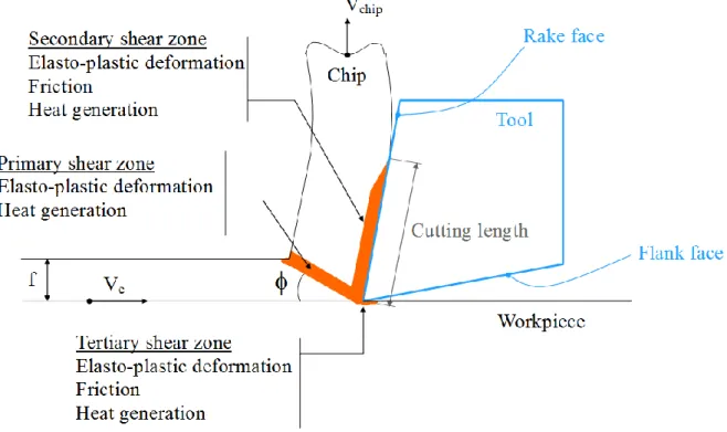
Heat generation in cutting was always a main topic studied in machining. The principal causes of heat generation during cutting are 1- the plastic deformation in the different shear zones, 2- the friction at the tool-chip interface and also at the tool-workpiece interface [1], Figure 1. The generated temperatures have a significant influence on the friction conditions at the chip and the tool-workpiece interfaces. Therefore, they have a consequence on the level of cutting forces. An increase of the workpiece temperature softens the material, thereby decreasing cutting forces and energy to cause further shear. The tool-chip contact temperature affects the seizure and the sliding conditions at this interface. They play an important role on the tool wear and then on the limitation of tool life. High
2 temperatures at the tool-workpiece interface accelerate the flank wear mechanisms and promote plastic deformation on the machined surface. That leads to a significant thermal load of the subsurface which may induce phase transformation, generate surface alterations and produce high tensile residual stresses which have a negative effect on the machined parts fatigue life.
Figure 1 - Heat sources in the orthogonal cutting process
It is possible to estimate the heat generated if the temperature may be measured; however, such a measurement is difficult [2]. The shear zones are extremely narrow; the temperatures as well as the gradients may reach high values. The chip prevents a direct observation of the tool rake face; two different bodies, i.e. chip and tool, are in sliding contact in a continuous or intermittent way [2]. Several techniques have been developed during the last eighty years in order to measure the temperature in various machining processes. They mainly use thermocouples (the embedded, dynamic or the chip–tool thermocouples), pyrometers and infrared thermography cameras. Komanduri and Hou [3], Abukhshim [2], and Davies et al. [4] reviewed previous works using these different measuring techniques. According to Abukhshim [2], the infrared thermography appears to be the most suitable in high speed machining applications. Main advantages are a fast response, no adverse effects on measured temperatures, no physical contact, and allowing measurements on objects, such as chips, which are difficult to access. As pointed out, a special care has to be taken regarding the measurement position to avoid chip obstruction. In addition the surface emissivity or at least the relation between measured digital level and the temperature should be known to perform accurate temperature measurements [5]. The surface emissivity depends on the material composition and may vary with
3 surface oxidation and roughness [6]. In the following, previous works using IR camera during different machining processes (orthogonal cutting, milling and drilling) are briefly presented.
Thermographic techniques were mainly used to measure temperature distribution during orthogonal cutting experiments [7]. Nevertheless, some researchers proposed measurement in complex machining operations such as milling [8] and even drilling [9].
Attention is here focused on the orthogonal cutting experiments. Young [10] used Infrared camera to measure the chip back temperature during orthogonal cutting of AISI 1045 steel. This author investigated the distribution of the temperature along the chip flow direction. Kwon et al. [11] investigated the rake face temperature distribution of the cutting tool inserts, after the feed was stopped; and an inverse estimation scheme was used to calculate temperature profiles. Usui et al. [12] examined the influence of tool flank wear on the whole temperature distribution within the cutting zone. Dinc et al. [13] used IR camera to measure the temperature distribution in the tool and valid prediction model.
Different cameras were employed. Some researchers used CCD cameras developed for the visible range, [13] and [14]. In comparison with the classical IR cameras, the cost of CCD cameras is lower but they only operate in the short wave infrared range; and they may only measure high temperatures. The proper measurement of the whole temperature range occurring in metal cutting needs a camera specifically developed for infrared observations [15].
This paper presents an experimental device using an IR camera and exposes an original experimental procedure for studying both the thermal and mechanical aspects of orthogonal cutting. It is thus shown how infrared thermography associated with the measurement of cutting forces can completely characterize an orthogonal cutting operation.
The measurements performed during the cutting tests, for various cutting conditions, were used to examine the validity of previous cutting models and provide the necessary elements for a new modeling approach, subject to further work. It is also shown that the device and the proposed procedure can be used to experimentally characterize the machinability of a material or the tool performance.
2 EXPERIMENTAL PROCEDURE 2.1 Experimental setup and IR Camera
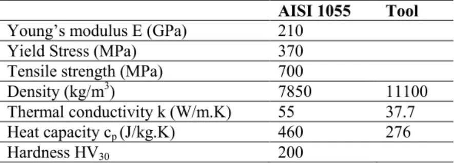
Orthogonal cutting tests of medium carbon steel AISI 1055 were carried out; Table 1 gives some of the main characteristics of the work material. The tool was a Sandvik Coromant TPUN 160308 coated carbide mounted on the toolholder TFPR 1603. The carbide grade was the referenced GC235 one, which heat capacity and thermal conductivity are given in Table 1. The values of rake angle and relief angle were respectively 6° and 5°.
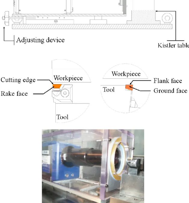
4 The experimental samples involved a tubular part with an outer diameter of 58 mm. The samples were integrated into the tool holder of the machine spindle; orthogonal cutting conditions were obtained by removing the end of the tubular part of the samples with a tool attached, through a special fixture, to a dynamometric table Kistler 9257A fixed on the machine table ( Figure 2). Lateral view of the cutting process (in a plane perpendicular to the cutting edge) was recorded with an infrared camera. This camera was adapted into CNC machine through a special device screwed on the machine table. In order to obtain thermal maps of the cutting tool and the chip and to observe the tool-chip interface, the tool insert was ground in a plane normal to the cutting edge. With this experimental setup and during cutting tests, both forces and temperature fields were measured.
The IR camera used in the experiments was a FLIR SC7000 equipped with a G3 lens. With this equipment, the full screen frame rate was up to 100 Hz, the field of view was about 9.5 mm x 7.5 mm, and the array size was 640 x 512 pixels providing a spatial resolution of about 15 µm x 15 µm / pixel. The focal distance was very short (i.e. 30 mm) thereby the camera was placed very close to the observed cutting zone, Figure 2. The temperature distribution commonly observed in metal cutting requires a large measuring range, i.e. from 0°C to 1500°C; then two configurations of the camera were used: the first one to measure the low temperature values from 0°C to 300°C, and the second one for higher temperature values from 300°C to 1500°C (this configuration consisted in the use of a spectral filter and with a 3.97 – 4.01 µm wavelength pass band filter at 60% transmission ratio). The Noise Equivalent Temperature Difference (NETD) was less than 25 mK for a black body at 25°C.
AISI 1055 Tool Young’s modulus E (GPa) 210
Yield Stress (MPa) 370
Tensile strength (MPa) 700
Density (kg/m3) 7850 11100
Thermal conductivity k (W/m.K) 55 37.7 Heat capacity cp (J/kg.K) 460 276
Hardness HV30 200
5
6 2.2 Operating conditions
The machining operation performed was an orthogonal cutting operation. Tool cutting edge angle R was
set at 90°. Tool inclination angle S was set at 0°. The machining operation is then performed with a
constant chip section and a constant cutting speed.
Cutting tests were performed in dry condition for many reasons: dry machining development is requested by manufacturing industries, coated carbide tool are designed for such cutting operations, and coolant prevents proper IR temperature measurement. Dry machining currently induces higher cutting temperatures and lower tool life.
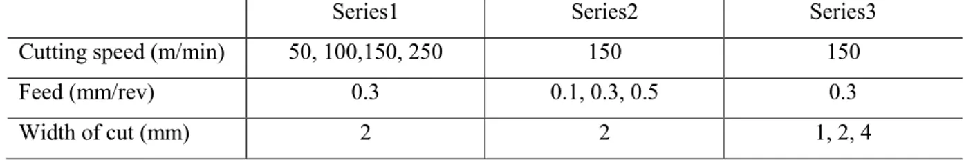
Experiments were carried out to observe the effects of cutting conditions, more precisely to study the respective influence of cutting speed Vc, feed f, and width of cut ap. Experiments are led using one-factor-at-a-time method. Three values for feed and width of cut were f and ap, chosen from a previous chip breaking analysis. For the cutting speed Vc, four values were selected; with all these values, the tool life was acceptable. Ten different cutting tests were performed at least twice due to the two measuring ranges of the IR camera. For the first series, only the value of the cutting speed has varied; for the second series, it was the speed that has been modified; and for the third, the depth of cut; see Table 2. The repeatability of the cutting process was verified with the repeatability test which lies at the three series intersection, it was carried out 10 times.
Series1 Series2 Series3
Cutting speed (m/min) 50, 100,150, 250 150 150
Feed (mm/rev) 0.3 0.1, 0.3, 0.5 0.3
Width of cut (mm) 2 2 1, 2, 4
Table 2 - Operating conditions 2.3 Calibration and processing
Emissivity
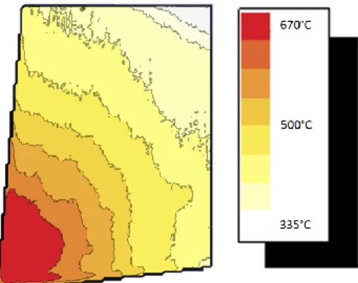
During experiments, two different materials (i.e. the work material and the cutting tool substrate) were in the field of view, each with its own emissivity. A specific setup was developed to calibrate the thermographic system in the various configurations, and preliminary tests were carried out in order to perform the conversion of digital levels into temperatures. These tests highlight the lower influence of emissivity on the calculated temperature value in the higher temperature range. Figure 3 is an example of the thermal field in the tool measured and determined after calibration. It can be noticed that the maximal temperature was reached, as expected, near the cutting edge for this orthogonal cutting operation.
7 Figure 3 - Thermal image obtained during the orthogonal process
Integration time
A full thermal map of the cutting zone requires the combination of images collected using the two camera configurations described previously, paragraph 2.1, and with several integration times. The integration time (IT) is the infrared thermography equivalent of the optical aperture time. A high integration time is, for a given configuration, adapted to the lower temperatures. An integration time from 40 to 400 µs leads to temperature ranges about 200-300°C or 300-1300°C depending on the configuration (with or without filter). An integration time down to a few µs leads respectively to temperature ranges about 200-300°C and above 800°C. The cutting process is a highly dynamic operation, high integration times give a blurred image; in the opposite, small integration times provide images with more accurate geometrical description. The main difficulty was then to define the different integration time values in regards to the temperature and to geometrical parameters to be measured such as shear angle or tool / chip contact length. Figure 4 presents examples of images obtained with two different integration times. Figure 4(a) gives the best estimation of the shear angle. Figure 4(b) gives the tool-chip contact length and the higher temperature values without sensor saturation.
(a) (b)
Figure 4 - Two images for several information
8 Automatic detection of the cutting tool contour,
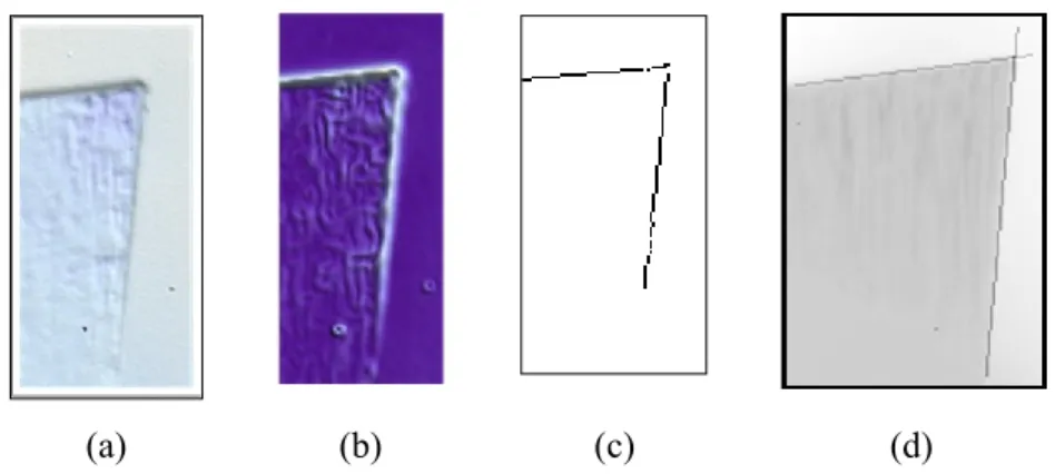
For a given set of cutting conditions, the whole temperature distribution measurement was obtained with two experiments, one for each configuration. In consequence, a special attention was paid to the repeatability, and then the experiments were carried out several times. Another difficulty was to locate with accuracy and objectivity the cutting edge on the camera recordings. In order to solve this problem, a Canny edge detection [17] was used. This method includes four stages: (1) windowing and identification of the cutting tool, (2) enhancement of the cutting tool contour, (3) extraction of the cutting tool contour, (4) and least square linear approximation for the acquired segmented contour, see Figure 5.
(a) (b) (c) (d)
Figure 5 - Automatic cutting tool detection
(a) windowing, (b) contour enhancement, (c) contour extraction, (d) least square linear approximation
This automatic detection process led to a cutting edge position error of about 45 µm. The error was smaller for the rake face position, as the detection error was smoothed through the linear approximation. In addition, with the cutting edge detection, the primary shear angle was easily measured on the thermal images; it was obtained from the line between the cutting edge and the outer workpiece - chip break point.
9 3 EXPERIMENTAL RESULTS
3.1 Cutting forces.
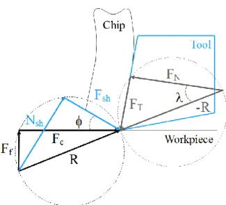
Figure 6 - Merchant forces decomposition
The forces along cutting and feed directions respectively Fc and Ff, (Figure 6)were measured using the
piezoelectric dynamometer. As the cutting operation was orthogonal, the third component was null; that was verified by measurements. Figure 7 gives typical cutting and feed forces signals, it may be noted that the chip section was constant after the tool engagement, and the cutting and feed forces were constant. Mean values and standard deviation were calculated for each cutting condition.
Figure 7 - Cutting forces for Vc = 150 m/min, f = 0.3mm/rev, and ap = 2 mm With these mean values, cutting pressures or specific energies kC and kf were then determined:
c c p F k f a (1) f f p
F
k
f a
(2)10 where the product of the feed f by the width of cut
a
p is considered as a proper estimation of the chip section. From the obtained results, it may be shown that these specific energies depend on the cutting parameters which are the cutting speed Vc, the feed f, and the width of cut ap. This dependenceis presented here through power laws:
3 1 2 0 n n n c c c p
k
k V f a
(3) 3 1 2 ' ' ' 0 n n n f f c pk
k V
f
a
(4)The values of the exponents and of the coefficients
k
c0 andk
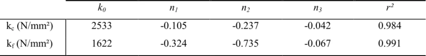
f0, which strongly depend on both tool and work material characteristics, were determined from experimental results through a linear regression, they are given in Table 3. Their relevancy was checked with the help of the correlation coefficient (see Table 3). They are both pretty high, up to 0.991 for kf.k0 n1 n2 n3 r²
kc (N/mm²) 2533 -0.105 -0.237 -0.042 0.984
kf (N/mm²) 1622 -0.324 -0.735 -0.067 0.991
Table 3 - Coefficients of the specific cutting energies laws
The trend seems also consistent: kc is mostly greater than kf; the increase of each cutting parameter generally tends to lower the specific energy values. The most influent parameter on kc or on kf is usually feed followed by cutting speed; the width of cut is the less influent, indeed the coefficients n3 and n’3 are the smaller ones in absolute value in Equations (3) and (4), see Table 3. Figure 8 gives the evolution of the cutting pressures with the most influent cutting parameters.
11 Figure 8 – Evolution of the cutting specific energy kc with cutting speed and feed
according to Equation (3)
AISI 1055 steel - 50 ≤ Vc ≤ 250 m/min – 0.1 ≤ f ≤ 0.5 mm/rev - ap = 2 mm.
3.2 Apparent friction coefficient
It is generally accepted that the tool-chip interface may be decomposed into two regions; in the first one the chip adheres to the tool rake face and is plastically sheared (sticking or seizure region), in the second one the chip slides on the rake face with friction (sliding region) [19]. Plastic deformation and friction are the main mechanisms at the tool-chip interface, they produce heat. Together, sticking and sliding regions are usually called secondary shear zone. In spite of this decomposition into two regions, an apparent friction coefficient is frequently calculated from the tangential
F
T and the normalN
F
components of forces acting on tool rake face in Figure 6. These two components are obtained from cutting and feed forces by using the Merchant diagram forces, Figure 6. An apparent friction coefficient may be defined by :tan
tan
tan
c f T N c fF
F
F
F
F
F
(5)In the same way as for the specific cutting energies, the apparent friction coefficient was determined from the measured cutting and feed forces. Its dependence on cutting conditions may be represented by the power law:
3 1 2 0 m m m c p
V
f
a
(6)12 Table 4 gives the numerical values of the coefficients of this law, the correlation coefficient was found around 0.99. The increase in cutting speed or feed leads to a decrease of the apparent friction coefficient. It depends slightly on width of cut, and at low feed and cutting speed values, it tends to 1. Figure 9 shows the evolution of the apparent friction coefficient with the cutting parameters.
m1 m2 m3 r²
0.767 -0.182 -0,431 -0.017 0.989
Table 4 - Coefficients of the apparent friction law
Figure 9 – Evolution of the apparent friction coefficient with cutting speed and feed according to Equation (6)
AISI 1055 steel - 50 ≤ Vc ≤ 250 m/min – 0.1 ≤ f ≤ 0.5 mm/rev - ap = 2 mm.
3.3 Shear angle and tool-chip contact length Chip formation
The observation and study of chip formation is a key factor to understand the cutting process and in a first stage the chip morphology was examined. It is well known that the chip morphology [18] is dependent on the cutting conditions, and Figure 10 gives images of chip formation for a feed about 0.3 mm/rev, a width of cut about 2 mm and various cutting speed values.
13 Figure 10 – Chip formation at various cutting speed values.
(Vc = 50, 100, 150 and 250 m/min, f = 0.3 mm/rev, ap = 2 mm)
At low cutting speed, the chip seems continuous, and as cutting speed increases it shows some localized shear bands which are characteristic of so-called serrated chips. Additionally, chip curling and chip breaking may be studied with the obtained images; however, that was not the subject of the present study. The emphasis was in the following rather put on shear angle and tool-chip contact length measurements presented in the following.
Shear angle
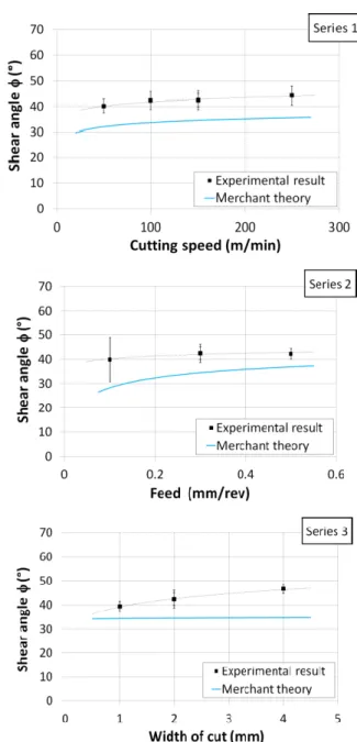
During experiments, the shear angle was clearly visible by using the appropriate integration time, Figure 4a. But even if the orthogonal cutting seemed to be stationnary, the IR recordings presented some variations of shear angle during cutting. In consequence, several shear angle values were extracted for each cutting conditions, and a mean value and standard deviation were calculated. The experimental shear angle mean values were compared to the Merchant’s shear angle values [20] obtained with the formula :
4 2
(7) is the friction angle determined from the experimental results through the Equation (5).14 Figure 11 - Comparison between experimental and calculated shear angle values.
Figure 11 presents the measured and the Merchant shear angles. It is noticeable that Merchant’s theory seems to underestimate the shear angle. According Equation (6-7), shear angle increases with cutting speed or feed; experimental results agree with these theoretical trends. Width of cut should not influence the shear angle; however experimental results highlight an increase of the shear angle with the width of cut.
Tool-chip contact length
With shear angle, tool-chip contact length is an important factor in the chip formation process. It plays a major role on the stress distributions in the shear zones and then on the mechanical and thermal tool loadings; as a consequence it has a significant influence on tool performance [21]. As it was explained previously, the tool-chip contact length is assumed to be decomposed into two regions: sticking region and sliding region. During the cutting process, the total tool-chip contact and its decomposition into
15 two regions control the amount of heat generated by plastic deformation and by friction in the secondary shear zone. The previous works have shown that the tool-chip contact length depends on cutting conditions, tool and coating materials, workpiece material. This dependence was taken into account through various models reviewed by Mativenga et al. [22] and Iqbal et al.[23]; they are presented in Table 5.
Authors
(Date) Model
Work material (Vc m/min)
Lee and Shaffer (1951) 1
2
sin[ 4
]
ct
l
sin
Mild steel Abuladze (1962) 1 2 12 [ (1 tan ) sec ]
ct
l
t
t
- Poletika (1969) 1 2 1[2.05
0.55]
ct
l
t
t
Iron, Steel, Copper, BronzeKato et al. (1972) Toropov and Ko (2003) 2
2
cl
t
EN AA 6061(1000) Copper(800) AISI 1045(300) AISI 304 (140)Tay et al. (1976) 1
sin[
]
cos
ct
l
sin
AISI 1016 (244) Vinogradov (1985) 1sin
4
cos[ 4
]
ct
l
sin
- Oxley (1989)
1sin
1
cos
3 1 2( 4
)
ct
nC
l
sin
nC
AISI 1016 (6-60)Zhang et al. (1991)
l
c
8.677 10
5t
10.5V
c0.065(90
)
0.733 AISI 1045 (300)Stephenson et al.
(1997)
l
c
0.485 0.0028
V
c AISI 1018 (82)Marinov (1999)
l
c
1.61
t
2
0,28
t
1 AISI 1020 (291)16 M. Zadshakoyan et al. (2013)
3 2 3 3 89.935 8.28 7.776 19.638 8.499 c c p p V l a f f f a f AISI 4140 (80-160)Table 5 - Models for the chip contact length from [23] and [24] t1 is the undeformed chip thickness, t2 the chip thickness,
the rake angle, the shear angle, and the friction angle.
It was difficult to measure, with a good accuracy, the contact length from the raw images recorded using the IR camera. At the end of the tool-chip interface, it was observed a significant oscillation of temperature with time; this clearly meant that the contact between the chip and the tool, at this point, became intermittent. For instance, Figure 12 gives the standard deviation of temperature along the contact measured for a particular set of cutting conditions during the stationary part of the experiment. The contact length was determined from the cutting edge to the beginning of the standard deviation increase.
Figure 12 - Example of contact length determination through standard deviation analysis (Vc = 150 m/min, f= 0.3 mm/rev, ap = 2 mm)
17 Figure 13 - Tool-chip contact length as a function of cutting conditions
Figure 13 summarizes the experimental results in comparison with models presented in Table 5. The overall trends are consistent with the previous works even if the contact length values may encounter some differences. As it was noticed by Sadik and Lindström [25], contact length increases if the feed increases; it seems independent from the width of cut. The feed is thus the cutting parameter with the greatest effect on contact length; this effect appears to be almost linear. The most relevant model seems to be the one developed by Zhang et al. [26]. He established this empirical model from cutting tests on a similar work material (AISI 1045); however the used tool was quite different since cutting edge was chamfered.
18 3.4 Thermal steady state
Orthogonal cutting is often considered as a steady state problem. During experiments, the temperature recordings have generally shown a transient stage which then evolves towards a ‘steady state’; however, this was not a strictly-speaking steady state [27]. Indeed, during the material removal process, the length of the sample was continuously decreasing, the thermal boundary conditions were then changing and the generated heat was accumulated at the top of the sample.
In order to approach this steady state, some observations were made with a virtual probe to check temperature time evolution for a point located at 0.6 mm far from the cutting edge within the tool-chip contact zone. This location was arbitrarily chosen. Results of these observations are shown, for several conditions, in Figure 14.
Vc = 150 m/min – ap = 2 mm f = 0.1 to 0.3 mm/rev
f = 0.3 mm/rev – ap = 2 mm Vc = 50 to 250 m/min Figure 14 - Temperature evolution function of cutting length
The measured temperature evolutions were approximated by a linear increasing function superposed to an exponential function:
0
01
1
x L
T T
e
B x
(5)T0, B and L0 are constants, and x represents the cutting length; they were determined for each cutting
test using a least square method. T0 may be considered as a temperature. B characterizes the linear
evolution of the temperature in the pseudo-steady state; when B is found small enough, the stationary assumption may be easily accepted. It should be noted that B was always small for all the cutting conditions tested in this study. L0 may be considered as a characteristic length: an estimation of the
minimum length to be cut before reaching the steady state. It may be useful to determine the lowest duration of a cutting test. These parameters have been estimated for each cutting test performed. It has been observed that the value of these parameters depends on the cutting conditions, i.e. values for Vc, f and ap. The values of T0, B and L0 have been processed to provide an empirical model. This model
shows how the cutting conditions induce variations on A, B and L0 Figure 15. Once more cutting
19 Figure 15 - Parameters for the temperature evolution versus cutting length, Equation (5) An increase in both cutting speed and feed induces an increase in T0 even if feed is clearly predominant
(since an increase of feed in a ratio from 1 to 5 induces an T0 increase about 40% while a similar increase
in cutting speed barely induces a slight T0 increase of about 10%). On the contrary L0 mainly depends
on cutting speed (since an increase of cutting speed in a ratio from 1 to 5 induces an L0 increase of about
200% while a similar increase in feed barely induces a slight L0 decrease of about 20%). Cutting tests
performed at low cutting speed should be then long enough if steady state is to be reached. All the experiments presented in the following have been made with a cutting length greater than 3 times L0.
3.5 Mean temperature along tool chip contact length
The data processing begins with an analysis of the global values such as the so-called “cutting temperature”, i.e. the mean temperature along the tool chip contact zone. Cutting temperature was often measured using the tool-workpiece thermocouple system [3], this technique was supposed to provide an image of the mean temperature. Here the objective is to obtain the evolution with cutting speed and feed of this interface mean temperature. The experimental values were determined from the measured temperature distribution along the tool-chip interface for a cutting length of 3 L0. The cutting
specific energy kc, the mean temperature and the temperature range at the tool-chip interface have been
20 (a)
f = 0.3 mm/rev – ap = 2 mm
(b)
Vc = 150 m/min – ap = 2 mm Figure 16 - Mean temperature evolution with cutting speed (a) and with feed (b).
Even if the cutting specific energy kc decreases with the increasing values of cutting speed and feed,
the cutting temperature increases. There are numerous results in the literature which confirm this tendency; it may be explained by the following facts : (1) more heat is being generated in the shear zones, (2) and/or is concentrated in a small area, (3) an/or less heat is being dissipated, as it was reported by Bacci da Silva and Wallbank [28]. Dimensional analysis applied to cutting highlights that the cutting temperature should be inversely proportional to the specific cutting energy kc and the root mean square of the cutting speed and feed [29].
3.6 Temperature fields
Figure 17 gives 2D thermal maps of the tool recorded for various cutting conditions. The evolution of the temperature fields versus cutting speed is first discussed. When cutting speed increases, the temperatures and the gradients both increase. It is also interesting to dwell on the flank face temperature distribution; the thermal gradient along the flank face in the vicinity of the tool edge seems to increase with the cutting speed. The smaller value of feed, 0.3 mm/rev., leads to the higher temperature gradients and to a reduced thermally affected area on the flank face. The flank temperature distribution has a direct effect on flank wear and has a consequence on the machined surface temperature. Depending on work material and cutting conditions, the machined surface and subsurface may be thermally affected and as a consequence tensile residual stresses may be induced, they have a negative influence on the components durability.
21 (a) (b) (c)
f = 0.3 mm/rev, ap = 2 mm
(a) Vc = 50, (b) Vc = 100 and (c) Vc = 250 m/min
Vc=150 m/min – ap = 2 mm
(d) f = 0.3mm/rev. (e) f = 0.5mm/rev.
Figure 17 - Temperature fields in the tool for various cutting conditions. 3.7 Temperature distribution along the tool-chip interface
It is well known that the temperature and its distribution along tool-chip interface affect the chip formation process through their effect on shearing properties of the work material ; their effect on friction characteristics in the sliding zone of this contact region, and they have significant influence on the tool wear mechanisms. The so-called cutting temperature, measurements of which were presented in paragraph 3.5, is not sufficient to refine metal cutting models or predict local tool wear rate.
22 f = 0.3 mm/rev – ap = 2 mm Vc = 150 m/min – ap = 2 mm
Vc = 150 m/min – f = 0.3 mm/rev
Figure 18 – Temperature distribution at tool – chip interface
Figure 18 shows the local temperature distribution for various cutting conditions. The global shapes are consistent with previous results collected using thermocouples [30] or pyrometers [31] or infrared camera [6]. The temperature reaches its maximum value in the vicinity of the cutting edge and is then decreasing up to the end of the tool-chip contact. Cutting conditions have a direct impact on the global level and on the location of the maximum temperature; when cutting speed, or feed and or width of cut increase, the temperature level increases and the location of the peak temperature moves away from the cutting edge. It appears that the feed has the most important effect on temperature distribution at the tool-chip interface; the effect of width of cut is reduced.
4. EXPERIMENTAL REMARKS AND FUTURE TRENDS
Similar experimental devices have been presented by Arrazola and al. [7] or Dinc et al. [13]. The measured cutting forces were used to calculate the cutting specific energy and the mean friction coefficient at the tool-chip interface. Our approach proposes to process thermal images not only to get temperature distributions but also to determine shear angle and tool-chip contact length. Furthermore instantaneous temperature values are used to check the validity of steady-state assumption. In addition, it must be noted that all the data were acquired during the cutting tests; therefore the processing was minimal and required no more complex systems such as Quick Stop Test for Primary Shear Zone observation or Scanning Electron Microscope for tool-chip contact zone measurements.
23 After the cutting tests performed with the proposed experimental setup, the following remarks and conclusions can be drawn:
As expected, the mean or apparent friction coefficient at the tool-chip interface is a decreasing function of cutting speed and feed. It takes into account of the main mechanisms at the tool-chip interface which are sticking and sliding with friction.
It must be noted that, during the cutting process and for each set of cutting conditions, the shear angle oscillates around a mean value. This main shear angle appears to be higher than the one given by the Merchant model.
A specific and original technique was developed to get the value of contact length. It was based on the temperature oscillation at the end of tool-chip interface. For the dependence with cutting speed and feed, the same trends as those given by previous works, are retrieved. The obtained values are very close to those measured by Zhang [26] for similar steel.
From the thermal images of the cutting zone recorded for various cutting conditions, the Temperature fields in the tool, and the temperature distribution at the tool-chip interface were obtained.
From measured temperature evolution versus time it was possible to establish a quasi steady state. The temperature distributions measured at the beginning of this quasi steady-state were chosen for the comparison between the different cutting conditions.
Even if the cutting specific energy kc decreases with increasing values of cutting speed and
feed, the cutting temperature increases; many results in the literature confirm this tendency. Local temperature distributions along tool-chip interface were extracted from thermal images.
Global level and maximum temperature position vary with cutting conditions. As cutting speed and feed increase the maximum temperature moves away from the cutting edge and the mean temperature increases.
The influence of cutting conditions on several parameters the cutting process such as cutting forces, cutting temperature, shear angle, and contact length at the tool-chip interface, has been pointed out. It highlights the adequacy of this protocol with thermo-mechanical advanced investigations of the orthogonal cutting process.
The experimental study detailed in this paper should be understood as a proposal for further post-processing developments of IR data collected in machining. Results are currently coupled with a thermo mechanical analytical modelling of chip formation process. Prospects are wide: determination of local heat partition ratios in the tool-chip interface, evaluation of heat flux densities and then stress distributions at the tool-chip interface, prediction of tool wear rate.
24 4 CONCLUSIONS
An innovative experimental setup using an infrared camera as main device was proposed in the present paper. With the help of a multi component dynamometer, it was proven that this device is able to fully investigate an orthogonal cutting process. Cutting temperatures and cutting forces were measured; chip formation and tool-chip contact were observed and analyzed; making these experimental device and approach powerful.
To demonstrate the capability and the efficiency of the proposed device, cutting tests on a medium carbon steel AISI 1055 were carried out to study the respective influence of cutting conditions on the measurements and observations. All the cutting tests were performed twice, the repeatability was thus verified.
The proposed orthogonal cutting infrared thermography workbench appears as a very relevant tool to enrich the global and local knowledge on both mechanical and thermal aspects of cutting.
AKNOWLEDGMENTS
The authors would like to give a special thanks to Jeremy Bianchin, Daniel Boehm, Lionel Simon and Marc Borsenberger for their assistance in this work.
REFERENCES
[1] G. Le Coz, M. Marinescu, A. Devillez, D. Dudzinski, L. Velnom, Measuring temperature of rotating cutting tools: Application to MQL drilling and dry milling of aerospace alloys, Applied Thermal Engineering 36 (2012) 434-444.
[2] N.A. Abukhshim, P.T Mativenga, M.A. Sheikh, Heat generation and temperature prediction in metal cutting: A review and implications for high speed machining, International Journal of Machine Tools and Manufacture 46-7/8 (2006) 782-800.
[3] R. Komanduri, Z.B Hou, A review of the experimental techniques for the measurement of heat and temperatures generated in some manufacturing processes and tribology, Tribology International 34 (2001) 653-682.
[4] M.A Davies, T. Ueda, R. M’Saoubi, B. Mullany, A.L. Cooke, On the measurement of temperature in material removal processes, CIRP Annals 56-2 (2007) 581-604.
[5] G. Boothroyd, Photographic technique for the determination of metal cutting temperatures, British Journal of Applied Physics 12-5 (1961) 238-242.
25 [6] P.J. Arrazola, I. Arriola, M.A. Davies, A.L. Cooke , B.S. Dutterer, The effect of machinability on
thermal fields in orthogonal cutting of AISI 4140 steel, CIRP Annals 57-1 (2008) 65-68.
[7] P.J. Arrazola, I. Arriola, M.A. Davies, Analysis of the influence of tool type, coatings and machinability on the thermal fields in orthogonal machining of AISI 4140 steels, CIRP Annals 58-1 (2009) 85-88.
[8] M. Armendia, A. Garay, A. Villar, M.A. Davies, P.J. Arrazola, High bandwidth temperature measurement in interrupted cutting of difficult to machine materials, CIRP Annals 59-1 (2010) 97-100. [9] J. Pujana, A. Rivero, A. Celaya, L.N. López de Lacalle, Analysis of ultrasonic-assisted drilling of
Ti6Al4V, International Journal of Machine Tools and Manufacture 49-6 (2009) 500-508. [10] H.T. Young, Cutting temperature responses to flank wear, Wear 201(1996) 117-120.
[11] P. Kwon, T. Schiemann, R. Kountanya, An inverse estimation scheme to measure steady state tool chip interface temperatures using an infrared camera, International Journal of Machine Tools and Manufacture 41-7 (2001) 1015-1030.
[12] E. Usui, T. Shirakashi, T. Kitagawa, Analytical prediction of cutting tool wear, Wear 100 (1984) 129-151.
[13] C. Dinc, I. Lazoglu, A. Serpenguzel, Analysis of thermal fields in orthogonal machining with infrared imaging, Journal of Materials Processing Technology 198 (2008) 147–154.
[14] G. Sutter, L. Faure, A. Molinari, N. Ranc, V. Pina, An experimental technique for the measurement of temperature fields for the orthogonal cutting in high speed machining, International Journal of Machine Tools and Manufacture 43-7 (2003) 671–678.
[15] J. Pujana, P.J. Arrazola, R. M’Saoubi, H. Chandrasekaran, Analysis of the inverse identification of constitutive equations applied in orthogonal cutting process, International Journal of Machine Tools and Manufacture 47-14 (2007) 2153-2161.
[16] R.C Dewes, E. Ng, K.S. Chua, P.G. Newton, D.K. Aspinwall, Temperature measurement when high speed machining hardened mould/die steel, Journal of Manufacturing Technology 92 (1999) 293-301.
[17] J.F. Canny, Finding edges and lines in images, Massachusetts Inst. of Tech., Technical Report 720, Cambridge, USA, 1983.
[18] T.H.C Childs, K. Maekawa, T. Obikawa, Y. Yamane, Metal Machining: Theory and Applications, Arnold, London, UK, 1999.
[19] V.P Astakhov, Metal cutting mechanics, CRC Press LLC, Boca Raton, USA, 2000
[20] M.E. Merchant, Mechanics of the Metal Cutting Process. I. Orthogonal Cutting and a Type 2 Chip, Journal of Applied Physics 16-5 (1945) 267.
26 [21] H.G. Abuladze, Character and the length of tool-chip contact (Russian) in Proceedings of
Machinability of Heat-resistant and Titanium Alloys, Kuibyshev (1962) 68–78.
[22] P.T. Mativenga, N.A Abukhshim, M.A. Sheikh, B.K.K. Hon, An investigation of tool chip contact phenomena in high-speed turning using coated tools, Proc. IMechE Part B: J. Engineering Manufacture 220 (2006) 657-667.
[23] S.A Iqbal, P.T. Mativenga, M.A. Sheikh, Contact length prediction: mathematical models and effect of friction schemes on FEM simulation for conventional to HSM of AISI 1045 steel, Int. J. Machining and Machinability of Materials 3-1/2 (2008) 18-33.
[24] M. Zadshakoyan, V. Pourmostaghimi, Genetic equation for the prediction of tool–chip contact length in orthogonal cutting. Engineering Applications of Artificial Intelligence 26 (2013) 1725–1730. [25] M.I. Sadik, B. Lindström, The effect of restricted contact length on tool performance, Journal of
Materials Processing Technology 48 (1995) 275-282.
[26] H.T. Zhang, P.D. Liu, R.S. Hu, R.S A three-zone model and solution of shear angle in orthogonal machining, Wear 143 (1991) 29–43.
[27] D.A. Stephenson, T.C. Jen, A.S. Lavine, Cutting tool temperature in contour turning: transient analysis and experimental verification, Transactions of the ASME Journal of Manufacturing Science and Engineering 119 (1997) 494–501.
[28] M.B. Da Silva, J. Wallbank, Cutting temperature: prediction and measurement methods -a review, Journal of Materials Processing Technology 88 (1999) 195–202.
[29] Shaw M.C., Metal cutting principles, Oxford series on advanced manufacturing, Oxford University Press, New York, USA, 2005.
[30] K. Maekawa, Y. Nahano, T. Kitagawa, Finite Element Analysis of Thermal Behaviour in Metal Machining, JSME International Journal Ser. C 39-4 (1996) 864-870.
[31] O.D. Prins, The influence of wear on the temperature distribution at the rake face, Annals of the CIRP 19 (1971) 579-584.