Smart distance keeping: modeling and perspectives for embedded diagnosis

(1)

HAL Id: inria-00540819

https://hal.inria.fr/inria-00540819

Submitted on 29 Nov 2010

HAL is a multi-disciplinary open access

archive for the deposit and dissemination of

sci-entific research documents, whether they are

pub-lished or not. The documents may come from

teaching and research institutions in France or

abroad, or from public or private research centers.

L’archive ouverte pluridisciplinaire HAL, est

destinée au dépôt et à la diffusion de documents

scientifiques de niveau recherche, publiés ou non,

émanant des établissements d’enseignement et de

recherche français ou étrangers, des laboratoires

publics ou privés.

Smart distance keeping: modeling and perspectives for

embedded diagnosis

Hassan Shraïm, Othman Nasri, Philippe Dague, Olivier Héron, Mickael

Cartron

To cite this version:

Hassan Shraïm, Othman Nasri, Philippe Dague, Olivier Héron, Mickael Cartron. Smart distance

keep-ing: modeling and perspectives for embedded diagnosis. 1rst International Conference on Intelligent

Systems, Modelling and Simulation ISMS’10, Jan 2010, Liverpool, United Kingdom. �inria-00540819�

(2)

SMART DISTANCE KEEPING: MODELING AND PERSPECTIVES FOR

EMBEDDED DIAGNOSIS

Hassan Shraim

LRI, University of Paris-sud 11, CNRS & INRIA Saclay - ˆIle-de-France Bˆat 490, 91405 Orsay Cedex France

Email: hassan.shraim@gmail.com

Othman Nasri

Email: othman.nasri@lri.fr

Philippe Dague

Email: philippe.dague@lri.fr

Olivier Heron

CEA LIST, Saclay

91191 Gif-sur-Yvette cedex France Email: olivier.heron@cea.fr

Mickael Cartron

CEA LIST, Saclay

91191 Gif-sur-Yvette cedex France Email: mickael.cartron@cea.fr

Abstract—This paper presents a detailed description of an advanced Adaptive Cruise Control (ACC) system implemented on a Renault-Volvo Trucks vehicle. One of the main differences between this new system, which is called the Smart Distance Keeping (SDK), and the classical ACC is the choice of the safe distance. This later is the distance between the vehicle (with the ACC or the SDK system) and the front obstacle (which may be a vehicle). It is supposed fix in the case of the ACC, while variable in the case of the SDK. The variation of this distance (in the case of SDK) depends essentially on the relative velocity between the vehicle and the front obstacle. The choice of this distance influences the velocity regulation. The main contribution of this work is on the SDK system architecture, the design of its environment model, and the proposition of a detection and isolation strategy for some of the possible faults that may be produced on the system.

Keywords-Smart Distance Keeping (SDK), vehicle modeling, fault diagnosis.

I. INTRODUCTION

An increasing number of vehicles are being equipped with adaptive cruise control (ACC). This technology is substantially more complex than conventional cruise con-trol; ACC adjusts the brake and/or throttle, within limited ranges, to maintain a constant headway from any vehicle that intrudes upon the path of the driver’s vehicle. While ACC provides a potential safety benefit in helping drivers to maintain a constant speed and headway [1], as with other types of automation, there is the potential for misuse and disuse [2]. Adaptive cruise control (ACC) provides assistance to the driver in the task of longitudinal control of his vehicle during motorway driving. The system controls the accelerator, engine power train and vehicle brakes to maintain a desired time-gap to the vehicle ahead.

For ACC to be effective, drivers need to understand the capabilities of the technology, which include braking and sensor limitations. Based on this understanding, they must

be able to intervene when a given situation exceeds ACC capabilities. However, drivers have difficulties in understand-ing how ACC functions [3]. As a result, they tend to rely on the system inappropriately. For instance, [4] showed that drivers failed to intervene when approaching a stopped queue of vehicles because they believed that the ACC could effectively respond to the situation. [6] introduced an unexpected acceleration into the ACC system during routine driving conditions, which resulted in a collision 33 percent of the time. Whether or not drivers can respond effectively when automation fails depends on their understanding of the type of failure that occurs and the context in which it occurs [5].

To ensure safe and effective use, ACC limits of operation should be identifiable and interpretable [7]. One approach to help drivers detect and respond to these limits is to match the limits of the ACC algorithm to the natural boundaries drivers use to switch between car-following and active braking behaviors, as defined by environmental cues [e.g. time headway (THW) and time to collision (TTC)].

Essentially, this means matching the function of the ACC to the way drivers perform the task of following other vehi-cles [7]. Individual differences in driving behavior, however, would require some degree of tuning of the ACC algorithm to individual drivers.

The SDK must be understood as a function to enhance the driver’s capability to manage his longitudinal environment, and is dedicated to a use on highways or expressways (straight line, low curvatures, one-way roads). The SDK is based on the immediate front environment sensing on one hand, and on the automated management of the truck lon-gitudinal actuators (brakes, engine, gearbox), all this being monitored and controllable at any time by the driver through the in-cabin human machine interface and the conventional driving commands (pedals, switches).

(3)

Sensor outputs should always be checked to ensure that they are within their expected operating range. Simple checks on the recent rate of change or variance of the output can also be incorporated. Faults which cause the sensor to have an offset or altered gain will affect the control system but may not be detected by this first level approach.

The traditional approach to sensor fault checking is to include hardware redundancy for sensors. If two sensors measuring the same quantity disagree, there is likely to be a fault in one of them, and if three or more measurements are available, the fault is likely to be in the sensor which disagrees most.

The high cost of providing direct hardware redundancy for sensors has led to the development of analytic redundancy techniques. Conceptually, this equates to creating virtual sensors from other available measurements, to compare with the one being monitored. Analytic redundancy is used in available passenger car control systems.

The paper is structured as: first we begin by a general description and modeling of the SDK controller with its environment system. The modeling in this work includes a simplified mathematical model of the wheels and the engine. Then, a strategy for the detection and the isolation of the some of the possible faults that may be produced on the overall system is shown. Finally test scenarios and conclusion are presented.

II. SYSTEM DESCRIPTION AND MODELING

A. SDK System

In our work, we are interested on the modeling and the diagnosis of the SDK system. On the diagnosis part, we con-centrate on the sensors fault diagnosis (truck velocity sensor, wheels angular velocity sensors, radar, engine sensors). We suppose during this study that no faults may be produced on the bus CAN or on coding the algorithms (software).

The main architecture of the global system can be rep-resented by figure 1. As shown in this figure, the global SDK system may be decomposed into two main parts, the SDK controller, and the SDK environment model. The main function of the SDK controller is to:

∙ find the minimal distance between the truck and the

front object,

∙ find the acceleration (deceleration) needed to realize the

correct functioning of the SDK system,

∙ use a control algorithm to control the engine.

Inputs to the controller:

∙ relative velocity between the SDK vehicle and the front

vehicle,

∙ distance between the SDK vehicle and the front vehicle,

∙ type of the front object (moving or not moving object),

∙ velocity of the SDK vehicle which may be found by

one of the following ways:

V c V e l o c i t y ( T r u c k ) S D K A L G O R I T H M - F i n d t h e m i n i m a l s a f e d i s t a n c e b e t w e e n t h e t r u c k a n d t h e f r o n t o b j e c t . - F i n d t h e a c c e l a r a t i o n ( d e c e l e r a t i o n ) n e e d e d t o r e a l i s e t h e c o r r e c t i o n f o n c t i o n n i n g t h e S D K f u n c t i o n . - U s e a c o n t r o l a l g o r i t h m e t o c o n t r o l t h e e n g i n e C o n t r o l s i g n a l t o t h e i n j e c t i o n E C U R a d a r 3 2 1 1 : R e l a t i v e v e l o c i t y ( t r u c k - f r o n t o b j e c t ) 2 : D i s t a n c e ( t r u c k - f r o n t o b j e c t ) 3 : T y p e o f t h e f r o n t o b j e c t

Figure 1. SDK system: algorithm and environment

– a velocity sensor (Tachograph, or from the

trans-mission system),

– the average value of wheels angular velocity

mea-surements.

Outputs from the controller:

∙ control of the injection system,

∙ information sent to the Human Machine Interface about

the status of the SDK system.

By showing this architecture, we see that the decision of the SDK controller depends essentially on the data issued from some sensors, which means, any faulty data, will influence the SDK system decision.

In order to avoid as maximum as possible the faulty data propagation, we analyze in this work the following element: the radar, the wheel, the engine, and the communication buses.

1) The Radar: The SDK needs to be informed about the

front object presence, and about its relative position and velocity. Within this work, the sensor is a 3 beam Doppler effect ARS100 Radar. This radar monitors the traffic in front of the vehicle using three stationary independent millimetre wave radar.

Moving and stationary objects are detected and their distance and relative velocity are measured and processed sixteen times per second.

Due to its physical nature, the radar sensor is offering ex-cellent performance characteristics even in adverse weather conditions.

Since the data issued from the radar depends on the external object, then in order to realize any simulation, several scenarios should be prepared for the movement SDK vehicle and the front object. In this work, we suppose that the distance and the relative velocity between the SDK vehicle and the front vehicle are inputs to the system (depending on the scenarios that we are choosing).

(4)

2) The Wheels: Wheel angular velocity is one of the

important inputs to the SDK controller. Based on the angular velocities (six wheels), the linear truck velocity is calculated. In this part, the wheel rotational dynamics are presented. By applying Newton’s Law to the dynamics of the wheels, we find:

𝐼𝑤𝑖𝑤˙𝑖 = 𝑅𝑖𝐹𝑋𝑖+ 𝑇 𝑜𝑟𝑞𝑢𝑒(𝑚𝑖) − 𝑇 𝑜𝑟𝑞𝑢𝑒(𝑏𝑖) (1)

Where 𝐼𝑤𝑖 is the moment of inertia of the wheel number

𝑖, 𝑅𝑖 is the effective radius, 𝑤𝑖 is the angular velocity of

the wheel, 𝑇 𝑜𝑟𝑞𝑢𝑒(𝑚𝑖) is the applied tractive torque, and

𝑇 𝑜𝑟𝑞𝑢𝑒(𝑏𝑖) is the braking torque.

B. Motor and Power Train

Modern diesel engines are essentially decomposed into several subsystems [10]: the exhaust manifold, the intake manifold, the injection (common rail), the engine with moving solids (rods, pistons, cylinders ...), the turbo charge. Each of these subsystems can be modeled separately, but for some of these subsystems it is difficult to develop analytical models, so static maps based on the knowledge about the system may be used.

The presented problem in this section is to develop a simplified model for the diesel engine (see figure 2) used by the SDK. Based on [10], the dynamics of motor rotation is given by (2).

𝐽𝑒𝑤˙𝑒(𝑡) = 𝑀𝑖𝑛𝑑(𝑡 − 𝜏𝑖) − 𝑀𝑓(𝑡) − 𝑀𝑙𝑜𝑎𝑑(𝑡) (2)

Where 𝑤𝑒 is the crank shaft angular velocity, 𝑀𝑖𝑛𝑑 is the

indicated torque, 𝜏𝑖is the delay, 𝑀𝑓(𝑡) is the friction torque,

𝑀𝑙𝑜𝑎𝑑 is the torque due to the load, and 𝐽𝑒is the effective

inertia of the engine.

In this work, the transmission system is represented as in the figure 3. For simplification purposes, the ”Transmission System” block is composed only of several constants, de-pending on the gearbox state.

1) The Admission and Intake Manifold: The temperature

𝑇𝑖𝑚 of the intake manifold is assumed to remain constant

due to the intercooler. Therefore, the analysis will be based on essentially on the variation of the pressure. In this study,

the input flow is characterized by the output flow 𝑃𝑖𝑚of the

compressor. In this study, the input flow is characterized by

the output flow𝑚˙𝑐 of the compressor (see equation (3)).

˙ 𝑃𝑖𝑚+ 𝜏𝑣𝑉𝑑𝑁𝑒 120𝑉𝑖𝑚 𝑃𝑖𝑚= ˙𝑚𝑐 𝑅𝑇𝑖𝑚 𝑉𝑚 (3)

Where 𝑉𝑖𝑚 is the volume of the intake manifold, 𝜏𝑣 is the

volumic efficiency, 𝑉𝑑is the exchange volume in the engine,

˙

𝑚𝑐 is the rotational velocity of the engine in rpm(𝑁𝑒 =

60𝑤𝑒 2𝜋 ). O U T L E T M A N I F O L D I N L E T M A N I F O L D B R A K I N G L O A D I N J E C T O R C O N T R O L S I G N A L S T O T H E I N J E C T O R S ( N ) C Y L I N D E R P R E S S U R E S E N S O R F U E L P R E S S U R E S E N S O R S E N S O R S F O R T E M P E R U T U R E A N D F L O W C R A N K S H A F T A N G U L A R P O S I T I O N , V E L O C I T Y S E N S O R E N G I N E R E G I M E S E N S O R F U E L T E M P E R A T U R E S E N S O R C O M P R E S S O R T U R B I N E A T M O S P H E R I C P R E S S U R E S E N S O R

Figure 2. Engine Architecture, [10]

G e a r b o x s t a t e ( a c t u a l g e a r n u m b e r ) T r a n s m i s s i o n s y s t e m A n g u l a r v e l o c i t y , a n d m o t o r t o r q u e s e n t t o t h e w h e e l s C r a n k s h a f t a n g u l a r v e l o c i t y

Figure 3. Transmission block

2) The Indicated Torque 𝑀𝑖𝑛𝑑: In order to calculate the

indicated torque, we should calculate firstly the indicated efficiency. Normally, this efficiency is a specific character-istic to the engine and it is found from empirical data. This efficiency is higher when the mixture is light, and it may be approximated by (4).

𝜇𝑖𝑛𝑑= 𝑎 + 𝑏𝜆 + 𝑐𝜆2 (4)

The coefficients (𝑎, 𝑏, 𝑐) are found by identification (three different tests have been made) and 𝜆 is defined by (5).

𝜆=

𝑃𝑖𝑚𝑤𝑒𝑉𝑑

4𝜋𝑅 𝜏𝑣

𝑇𝑖𝑚𝑚˙𝑓

(5)

Then the indicated torque 𝑀𝑖𝑛𝑑 can be found as follows:

𝑀𝑖𝑛𝑑= 𝑚𝑓𝑝𝑐𝑖𝜇𝑖𝑛𝑑 (6)

𝑝𝑐𝑖 is a characteristic for the diesel(40000000𝐽𝐾𝑔−1).

3) The Injection: The injection system controls the

quan-tity of fuel that will be introduced into the combustion chamber. The mixture Air/fuel should be capable to auto ignited by the effect of temperature and the high pressure. The calorific power of combustion is related to the quantity of fuel injected. The following model gives the flow of fuel

𝑚𝑓 in function of the accelerator pedal 𝑥𝑝 and the engine

speed (see equations (7) and (8)) [10].

˙

𝑚𝑓 = 𝑖0+ Δ ˙𝑚(𝑆𝐷𝐾)+ Δ ˙𝑚𝑓 (7)

Δ ˙𝑚𝑓 = 𝑤𝑒(𝑖1+ 𝑖 − 2𝑥𝑝+ 𝑖3𝑥2𝑝+ 𝑖4𝑤𝑒) (8)

Where 𝑖0 characterizes the minimal injection flow (greater

than zero, when the engine is idle), 𝑚𝑓models the variations

of the flow around, 𝑖0, 𝑖1, ..., 𝑖4are constants.

4) The Friction Torque 𝑀𝑓: The friction torque may be

calculated by (9).

𝑀𝑓 =

(𝑐0+ 𝑐1𝑤𝑒+ 𝑐1𝑤2𝑒)𝑉𝑑

2𝜋𝑛𝑟 (9)

5) The Load Torque 𝑀𝑙𝑜𝑎𝑑: The torque 𝑀𝑙𝑜𝑎𝑑 depends

on the type of the road, the vehicle velocity, the turnings,... In this work we will suppose that this torque is input to the system and it has a constant value.

III. POSSIBLE FAULTS AND DIAGNOSIS STRATEGY

In this section, we present the possible faults that may be produced and diagnosis strategy realized.

A. Radar Data

1) Detection Performance: The basic data detection

re-quirement is to measure distance, relative speed, and reflec-tion signal amplitude of moving and stareflec-tionary objects in three beams. Angular position is calculated by the interpo-lation algorithms based on signal levels in adjacent beams.

2) Several Scenarios For the Radar Fault Detection Anal-ysis:

i. First: if the radar is faulty and doesn’t detect any object. So, without the help of another device, we can do nothing.

ii. Second: if the radar works but gives incorrect dis-tances (with a certain shift of 𝑥 meters): for example

(150 𝑚 → 150 − 𝑥 𝑚) where 𝑥 is a constant term,

then, we cannot detect this fault.

iii. Third: if the relative velocity and the distance between the vehicles are measured separately (two different measurement tools), then it is important to check at each period (for example 2 seconds) if the variation in the distance corresponds to the variation in the relative

velocity. If there is a difference then we say that there is a fault.

Ex: suppose that we initially have the relative velocity

𝑉𝑟𝑒𝑙 and the distance 𝑑 between the SDK truck and

the front vehicle 𝐴𝑉 see figure 4, so if we consider that the period (that we choose for checking) is equal to2 seconds, then we should obtain

𝑑(𝑡) − 𝑑(𝑡 − 2) = 2 ∗ 𝐴𝑣𝑒𝑟𝑎(𝑉𝑟𝑒𝑙)

Where 𝐴𝑣𝑒𝑟𝑎(𝑉𝑟𝑒𝑙) is the average value of 𝑉𝑟𝑒𝑙in the

period of 2 seconds.

iv. Fourth: Suppose that the radar was detecting a front

𝐴𝑉 ; vehicle (see figure 4).

S D K A V

d

Figure 4. SDK Vehicle and the front vehicle AV

Let 𝑉𝑟𝑒𝑙 be the relative velocity between the two vehicles

then: 𝑉𝑟𝑒𝑙 = 𝑉𝑎𝑣−𝑉 . As we have shown before, the relative

velocity is a measurement given by the radar. And also, the SDK vehicle velocity 𝑉 is measured from other sensors (wheels angular velocities or vehicle velocity), then we can find the velocity of the 𝐴𝑉 vehicle.

Getting the velocity of the front vehicle we can analyse as follows:

If there is a strong sudden variation (and then its acceleration (deceleration) is not realistic) then we have one of the two following cases:

i. there is a fault in the radar sensor,

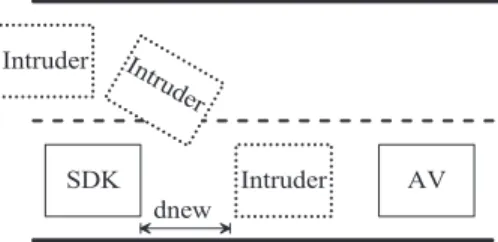
ii. the value of the SDK vehicle velocity is faulty, iii. an intruder vehicle comes in front of the SDK vehicle

(see figure 5).

In all the above cases, it is important to observe the velocity of the AV vehicle for several points before taking any decision. I n t r u d e r S D K A V I n t r u d e r _{I n t r} u d e_r d n e w

Figure 5. SDK Vehicle and the front vehicle AV with intruders (vehicles) In some of the above cases, the calculation of the AV vehicle acceleration (deceleration), may give a non realistic

(6)

values. A study about the maximum (minimum) possible acceleration (deceleration) can be given as follows:

∣𝑎𝑥∣𝑚𝑎𝑥 = max ∣ ∑ 𝐹_𝑥𝑖𝑗 𝑚 ∣ = max ∣ 𝜇.𝑁𝑧 𝑚 ∣ = max ∣ 𝜇.𝑚.𝑔 𝑚 ∣ ≤ 𝜇𝑚𝑎𝑥.𝑔 (10)

A maximum friction coefficient (𝜇𝑚𝑎𝑥) determines

maxi-mum acceleration or deceleration. It can be estimated using sliding modes techniques as follows (see the following section). Then if a non realistic acceleration (deceleration) value is found, then if there is no intruder vehicle, we can suppose that there is radar fault.

The overall diagnosis block for the Radar can be repre-sented by the figure 6.

D i s t a n c e f r o m t h e r a d a r s e n s o r s R e l a t i v e v e l o c i t y f r o m t h e r a d a r s e n s o r s T r u c k v e l o c i t y F r o m a n o t h e r d i a g n o s i s b l o c k a s i g n a l p r e c e s i n g i f t h e t r u c k v e l o c i t y i s f a u l t y o r n o t R a d a r f a u l t d i a g n o s i s b l o c k V e l o c i t y o f t h e f r o n t v e h i c l e D i a g n o s i s d e c i s i o n

Figure 6. Radar fault diagnosis block

B. 𝜇𝑚𝑎𝑥 Estimation

In order to estimate 𝜇𝑚𝑎𝑥, sliding modes observers can

be applied. A hierarchical observer is needed for this esti-mation. In the first step, an observer based on the dynamical equation of the wheels should be developed. This observer takes as an input the applied motor torque (which is es-timated statically (existing maps)) and the braking torque, which can be easily found based on the hydraulic pressure sent to the wheels [8]. Then, in parallel to this observer, a sliding modes observer is used to estimate the vertical forces. This observer is based on the suspension system modeling [9]. Then by calculating the longitudinal force and the vertical force we apply the following formula to estimate the adherence coefficient:

𝜇𝑚𝑎𝑥>

max(∑𝑛_𝑖=1𝐹𝑥𝑖)

min(∑𝑛_𝑖=1𝐹𝑧𝑖)

(11)

Where 𝑛 is the number of the wheels (equals to 6), 𝐹𝑥𝑖 and

𝐹𝑧𝑖 are respectively the longitudinal and the vertical forces

applied at the wheel 𝑖.

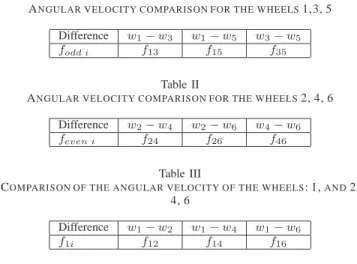
Table I

ANGULAR VELOCITY COMPARISON FOR THE WHEELS1,3, 5 Difference 𝑤1− 𝑤3 𝑤1− 𝑤5 𝑤3− 𝑤5

𝑓𝑜𝑑𝑑 𝑖 𝑓13 𝑓15 𝑓35

Table II

ANGULAR VELOCITY COMPARISON FOR THE WHEELS2, 4, 6 Difference 𝑤2− 𝑤4 𝑤2− 𝑤6 𝑤4− 𝑤6

𝑓𝑒𝑣𝑒𝑛 𝑖 𝑓24 𝑓26 𝑓46

Table III

COMPARISON OF THE ANGULAR VELOCITY OF THE WHEELS: 1,AND2, 4, 6

Difference 𝑤1− 𝑤2 𝑤1− 𝑤4 𝑤1− 𝑤6

𝑓1𝑖 𝑓12 𝑓14 𝑓16

C. Truck Velocity

The truck velocity used in the embedded SDK system is found by calculating the mean value of the wheels angular velocities. The truck velocity is an important decision term for the SDK controller. So, in order to ensure that the truck velocity value is not faulty, we analyze the rotational velocity value of each wheel. A simple fault detection strategy (based on the comparison between wheels velocities) aiming to detect wheels angular velocities sensors fault is proposed. To realise this study, two important steps are done:

1) A Simulator for the Truck Model: A Matlab Simulink

simulator representing the truck model is prepared. All the equations presented previously in the paper are coded in this simulator. The angular velocities of the wheels are found by equations 1, where the motor torque is found based on the angular velocity of the crank shaft (by a static map). The braking torque also is an input to these equations. This torque can be calculated based on the hydraulic brake pressure sent to the wheel [8].

2) A Detection Strategy: Two cases are considered based

on steering angle:

i. Case of straight line motion: In this case, we suppose that the angular velocities of the six wheels should be approximately equal. Then in order to apply this strategy, we suppose that we have two groups: group 1 (for the wheels: 1, 3, 5), and group 2 (for the wheels: 2, 4, 6), and we calculate the differences in the angular velocities as shown in table I and table II. Then if

(𝑤𝑖 − 𝑤𝑗) < 𝜖, then we suppose that there is no

fault, and 𝑓𝑖𝑗 = 0, else we have a fault and 𝑓𝑖𝑗 = 1.

To localise the fault in the case of 𝑓𝑖𝑗 = 1, a small

algorithm is realized. This algorithm is able to localise from 1 to 4 faults. In the case of more than four, it gives a signal that all the wheels are faulty.

The realization of this algorithm is based on the tables 1, 2, 3, 4, 5. By completing these tables, the localisation of the fault will be evident.

(7)

Table IV

𝑓3𝑖 𝑓32 𝑓34 𝑓36

Table V

𝑓5𝑖 𝑓52 𝑓54 𝑓56

ii. Case of a curve motion: In this case, we follow the same strategy proposed in the previous case, with the five tables, but the main difference here, in the case of the curve, is when we compare a wheel in group 1 (for the wheels : 1, 3, 5) to a wheel in group 2 (for the wheels: 2, 4, 6, we should take in consideration a small difference that can be calculated geometrically based on the Ackerman angle theory and based essentially on the steering angle. And then we should replace 𝜖 by 𝜖′_.

In addition to the decision about faulty sensors, the truck real velocity can be also calculated in this algorithm, this velocity is the actual real velocity which is approximated based on the non faulty sensors in the case that the number of the faulty sensors is less than four.

IV. TEST CONDITIONS AND SIMULATION ENVIRONMENT

First, mathematical models are validated by the company Renault-Volvo Trucks (Lyon Section in France). Several tests have been realized and the results were reasonable. Then, the above functions and algorithms are coded in the C language and implemented in the microcontroller card (prepared by the company Serma Engineering). The supervisor’s role is to treat all CAN messages, sent to it in CANoe. From these messages, it retrieves information required for diagnosis, applies the algorithm developed by the global ECU and sends to other ECUs through Can-bus network the diagnostic results and the counter-reactions. In addition, in order to visualize the diagnosis results and the supervisor activity, a PC interface is used by RS232 link. It allows communication between the supervisor and a HMI that displays progressively the information provided by the supervisor.

V. CONCLUSIONS

In this work, we have presented the architecture of the SDK system, with simplified models for the Engine and the wheels. A simplified strategy for the faults detection and isolation is also presented. Based on the analysis that we have done, we conclude that the proposed strategy for the detection and the isolation of faults (especially wheels

angular velocities) may improve the performance of the SDK system and increase its safety level.

REFERENCES

[1] Davis, L.C. ’Effect of Adaptive Cruise Control Systems on Traffic Flow’. Physical Review E, 69(6), 2004.

[2] Parasuraman R. Riley V. ’Humans and Automation: Use, Misuse, Disuse, Abuse’, Human Factors, 39(2), pp. 230-253, 1997.

[3] Stanton, N.A., Marsden, P. (1996). From fly-by-wire to drive-by-wire: Safety implications of automation in vehicles. Safety Science, 24(1), pp. 35-49, 1996.

[4] Nilsson, L. Safety effects of adaptive cruise control in critical traffic situations, Proceedings of the Second World Congress on Intelligent Transport Systems: Steps Forward, Vol. III, (Yokohama: VERTIS), pp. 1254-1259, 1995.

[5] Lee, J. D., See, K. A. ’Trust in technology: Designing for appropriate reliance’. Human Factors, 46(1), pp. 50-80, 2004. [6] Stanton, N.A., Young, M., McCaulder, B. ’Drive-by-wire: the case of driver workload and reclaiming control with adaptive cruise control’. Safety Science 27 (2), pp. 149159, 1997. [7] Goodrich, M.A., Boer, E.R., 2003. ’Model-based

human-centered task automation: a case study in ACC system de-sign’. IEEE Transactions on Systems, Man, and Cybernetics Part ASystems and Humans 33 (3),pp. 325336, 2003. [8] Shraim H., , ”Modeling, Estimation and control for vehicle

dynamics”, PhD Thesis, University Paul Czanne Aix Mar-seille III, 2007.

[9] Imine H. and Dolcemascolo V., ”Sliding Mode observers to heavy vehicle vertical forces estimation ”, IJHVS, Interna-tional Journal of Heavy Vehicle Systems, 2008, Vol. 15, No.1 pp. 53-64.

[10] Peysson F. , Noura H., Younes R., ’Diagnostic de d´efauts sur un moteur diesel’, CIFA06, 2006, Bordeaux, France.