Rotation, spectral variability, magnetic geometry and magnetosphere of the Of?p star CPD -28° 2561

arXiv:1411.7926v1 [astro-ph.SR] 28 Nov 2014

Rotation, spectral variability, magnetic geometry and

magnetosphere of the Of?p star CPD −28

◦

2561

⋆

G.A. Wade†

, R.H. Barb´a

, J. Grunhut

, F. Martins

, V. Petit

_{‡, J.O. Sundqvist}

,

R.H.D. Townsend

, N.R. Walborn

, E. Alecian

, E.J. Alfaro

, J. Ma´ız Apell´aniz

_{§, J.I. Arias}

,

R. Gamen

, N. Morrell

, Y. Naz´e

_{¶, A. Sota}

, A. ud-Doula

and the MiMeS Collaboration

1_{Department of Physics, Royal Military College of Canada, PO Box 17000 Station Forces, Kingston, ON, Canada K7K 7B4} 2_{Departamento de F´ısica, Universidad de La Serena, Av. Cisternas 1200 Norte, La Serena, Chile}

3_{European Southern Observatories, Karl-Schwarzschild-Str. 2, 85748, Garching, Germany}

4_{LUPM-UMR5299, CNRS & Universit´e Montpellier II, Place Eug`ene Bataillon, F-34095, Montpellier, France} 5_{Department of Physics and Astronomy, Bartol Research Institute, University of Delaware, Newark, DE 19716, USA} 6_{Institut f¨ur Astronomie und Astrophysik der Universit¨at M¨unchen, Scheinerstr. 1, D-81679 M¨unchen, Germany} 7_{Department of Astronomy, University of Wisconsin-Madison, 475 N Charter Street, Madison, WI 53706, USA} 8_{Space Telescope Science Institute, 3700 San Martin Drive, Baltimore, MD 21218, USA}

9_{UJF-Grenoble 1/CNRS-INSU, Institut de Plan `Etologie et d’Astrophysique de Grenoble (IPAG) UMR 5274, 38041, Grenoble, France} 10_{Instituto de Astrof´ısica de Andaluc´ıa-CSIC, Glorieta de la Astronom´ıa s/n, E-18008 Granada, Spain}

11_{Instituto de Astrof´ısica de La Plata (CCT La Plata-CONICET, Universidad Nacional de La Plata), Paseo del Bosque s/n, 1900 La Plata, Argentina} 12_{Las Campanas Observatory, Observatories of the Carnegie Institution of Washington, La Serena, Chile}

13_{FNRS-GAPHE, D´epartement AGO, Universit´e de Li`ege, All´ee du 6 Aoˆut 17, Bat. B5C, B4000-Li`ege, Belgium}

14_{Groupe d’Astrophysique des Hautes Energies, Institut d’Astrophysique et de G´eophysique, Universit´e de Li`ege, 17, All´ee du 6 Aoˆut, B5c, B-4000 Sart Tilman, Belgium} 15_{Penn State Worthington Scranton, Dunmore, PA 18512, USA}

Accepted . Received , in original form

ABSTRACT

We report magnetic and spectroscopic observations and modeling of the Of?p star CPD −28◦ _{2561. Using more than 75 new spectra, we have measured the equivalent width}

variations and examined the dynamic spectra of photospheric and wind-sensitive spectral lines. A period search results in an unambiguous 73.41 d variability period. High resolu-tion spectropolarimetric data analyzed using Least-Squares Deconvoluresolu-tion yield a Zeeman signature detected in the mean Stokes V profile corresponding to phase 0.5 of the spectral ephemeris. Interpreting the 73.41 d period as the stellar rotational period, we have phased the equivalent widths and inferred longitudinal field measurements. The phased magnetic data ex-hibit a weak sinusoidal variation, with maximum of about 565 G at phase 0.5, and a minimum of about -335 G at phase 0.0, with extrema approximately in phase with the (double-wave) Hα equivalent width variation. Modeling of the Hα equivalent width variation assuming a quasi-3D magnetospheric model produces a unique solution for the ambiguous couplet of in-clination and magnetic obliquity angles: (i, β) or (β, i) = (35◦_,90◦_{). Adopting either geometry,}

the longitudinal field variation yields a dipole polar intensity Bd = 2.6 ± 0.9 kG, consistent with that obtained from direct modelling of the Stokes V profiles. We derive a wind magnetic confinement parameter η_{∗ ≃ 100, leading to an Alfv´en radius R}A ≃ 3 − 5 R∗, and a Kepler

radius RK≃ 20 R∗. This supports a physical scenario in which the Hα emission and other line

variability have their origin in an oblique, co-rotating ’dynamical magnetosphere’ structure resulting from a magnetically channeled wind. Nevertheless, the details of the formation of spectral lines and their variability within this framework remain generally poorly understood. Key words: Stars : rotation – Stars: massive – Instrumentation : spectropolarimetry.

⋆ _{Based on observations obtained at the Canada-France-Hawaii Telescope}

(CFHT) which is operated by the National Research Council of Canada, the

Institut National des Sciences de l’Univers (INSU) of the Centre National de la Recherche Scientifique of France, and the University of Hawaii.

1 INTRODUCTION

The Of?p stars are mid-O-type stars identified by a number of pecu-liar observational properties. The classification was first introduced by Walborn (1972) according to the presence of C iii λ4650 emis-sion with a strength comparable to the neighbouring N iii lines. Well-studied Of?p stars are now known to exhibit recurrent, and apparently periodic, spectral variations (in Balmer, He i, C iii and Si iii lines), narrow P Cygni or emission components in the Balmer lines and He i lines, and UV wind lines weaker than those of typical Of supergiants (see Naz´e et al. 2010, and references therein).

Only 5 Galactic Of?p stars are known (Walborn et al. 2010): HD 108, HD 148937, HD 191612, NGC 1624-2 and

CPD −28◦ _{2561. Four of these stars - HD 108, HD 148937, HD}

191612 and NGC 1624-2 - have been studied in detail based on op-tical spectra, and in some cases UV spectra as well. In recent years, they have been carefully examined for the presence of magnetic fields (Donati et al. 2006; Martins et al. 2010; Wade et al. 2011, 2012a,b) and all have been clearly detected. It therefore appears that the particular spectral peculiarities that define the Of?p classi-fication are a consequence of their magnetism. Indeed, Hubrig et al. (2011, 2012) reported 4 FORS+VLT measurements of the

longitu-dinal magnetic field of CPD −28◦_{2561 at the few hundred G level,}

several of which correspond to detections at somewhat more than 3σ significance.

Like HD 108, HD 191612, HD 148937 and NGC 1624-2,

CPD −28◦_{2561 is a spectroscopic variable star (e.g. Walborn et al.}

2010). The spectrum of CPD −28◦ _{2561 was first described as a}

peculiar Of type by Walborn (1973) and Garrison, Hiltner & Schild (1977). Garrison et al. commented: ’Very peculiar spectrum. Car-bon (C iii λ4070) is strong, nitrogen weak. H and He ii lines are broad, while He i lines are sharp,’ Walborn classified the spec-trum as O6.5fp. The outstanding peculiarity was that although He ii

λ4686 emission was very strong, appropriate for an Of supergiant,

the N iii λ4640 emission was incompatibly not.

While Walborn (1973) announced HD 191612 as a new, third member of the Of?p class, it is significant that no such

associa-tion was made for CPD −28◦ _{2561. The reason was that no C iii}

λ_{4650 emission was detected in CPD −28}◦ _{2561, while a}

com-parable emission strength to that of N iii was the primary defin-ing Of?p characteristic. (Of course, it was subsequently discovered that the C iii emission disappears entirely at the minimum phase of HD 191612 (Walborn et al. 2004; Howarth et al. 2007; Wade et al. 2011)). It was not until the intensive OWN survey’s high-resolution

monitoring of CPD −28◦ _{2561 (Barb´a et al. 2010) revealed}

ex-treme variations in λ4686 and Balmer lines, analogous to those of HD 191612, that the association was made (Walborn et al. 2010)

and CPD −28◦_{2561 identified as an Of?p star.}

In this paper we perform a first detailed investigation of the

combined magnetic and variability properties of CPD −28◦ ₂₅₆₁

using an extensive spectroscopic and high-resolution spectropolari-metric dataset. In Sect. 2 we discuss the data acquired and the meth-ods of analysis used. In Sect. 3 we re-examine the physical proper-ties of the star, as well as its projected rotational velocity. In Sect. 4 we examine the spectral characteristics and variability, identifying periodic variability of the Hα and other emission and absorption lines and deriving the rotational period of the star. In Sect. 5 we

‡ Currently at Dept. of Physics & Space Sciences, Florida Institute of

Tech-nology, Melbourne, FL, USA

§ Currently at Centro de Astrobiolog´ıa, INTA-CSIC, Madrid, Spain. ¶ FNRS Research Associate

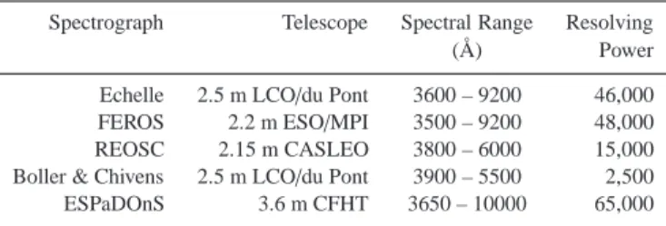
Table 1. Spectrographs used for the acquisition of CPD −28◦₂₅₆₁

spec-troscopy and spectropolarimetry.

Spectrograph Telescope Spectral Range Resolving

(Å) Power

Echelle 2.5 m LCO/du Pont 3600 – 9200 46,000 FEROS 2.2 m ESO/MPI 3500 – 9200 48,000

REOSC 2.15 m CASLEO 3800 – 6000 15,000

Boller & Chivens 2.5 m LCO/du Pont 3900 – 5500 2,500

ESPaDOnS 3.6 m CFHT 3650 – 10000 65,000

analyse in detail the magnetic data acquired at the Canada-France-Hawaii Telescope (CFHT). In Sect. 6 we employ the Hα EW varia-tion and CFHT magnetic data to constrain the stellar and magnetic geometry and the surface field strength. In Sect. 7 we derive the

magnetospheric properties of CPD −28◦ _{2561. Finally, in Sects.}

8 we summarize our results, and explore the implications of our study, particularly regarding the variability and other properties of

CPD −28◦_{2561, the confinement and structure of its stellar wind,}

and of the properties of the general class of Of?p stars.

2 OBSERVATIONS

2.1 Spectroscopic observations

Spectroscopic observations of CPD −28◦ _{2561 were obtained in}

the framework of two spectroscopic surveys: the High-resolution spectroscopic monitoring of Southern O and WN-type Stars (The ”OWN Survey”, Barb´a et al. 2010) and the Galactic O Star Spectro-scopic Survey (”GOSSS”, Ma´ız Apell´aniz et al. 2011) In the OWN Survey program, high-resolution and high signal-to-noise spectra are being acquired for a sample of 240 massive southern stars selected from the Galactic O Star Catalogue (GOSC version 1, Ma´ız-Apell´aniz et al. 2004). One of the goals is to determine pre-cise radial velocities in order to detect new binaries among these stars for which there is scarce or no indication of multiplicity. An additional goal is to detect possible spectral variations which can be related to multiplicity, the presence of magnetic fields,

pulsa-tion, or eruptive behaviour. CPD −28◦_{2561 was included early in}

the observed sample, and monitored systematically as large varia-tions in the intensity of the He ii λ4686 emission line were detected. The star was observed spectroscopically from three different loca-tions: Las Campanas Observatory (LCO), and La Silla Observa-tory (LSO), both in Chile, and Complejo Astron´omico El Leoncito (CASLEO), in Argentina, during 33 nights between 2006 and 2012. Seven spectrograms were obtained with an ´echelle spectro-graph attached to the 2.5 m LCO/du Pont telescope. The spec-tral resolving power is about 46,000. Twelve spectrograms were obtained with the FEROS ´echelle spectrograph attached to the 2.2 m ESO/MPI telescope. In this case, the spectral resolving power is about 48,000. Additionally, four spectrograms were obtained

with the REOSC ´echelle spectrograph1 _{attached to the 2.15 m}

CASLEO/Jorge Sahade telescope, with a resolving power of about 15,000. Thorium-Argon comparison lamp exposures were obtained before or after the science exposures. LCO and CASLEO ´echelle

1 _{Jointly built by REOSC and Li`ege Observatory, and on long-term loan} from the latter.

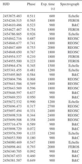
Table 2. Log of spectroscopic observations showing heliocentric Julian

Date, rotational phase according to Eq. (1), and exposure time. The column ’Spectrograph’ corresponds to the facilities described in Table 1.

HJD Phase Exp. time Spectrograph (s) 2453875.483 0.511 600 Echelle 2454246.515 0.565 1800 FEROS 2454610.486 0.523 900 B&C 2454627.467 0.754 1800 FEROS 2454786.865 0.926 900 Echelle 2454842.716 0.687 1800 REOSC 2454846.677 0.741 1800 REOSC 2454847.609 0.753 2000 REOSC 2454848.650 0.767 1800 REOSC 2454954.537 0.210 1800 FEROS 2454955.500 0.223 1800 FEROS 2454964.476 0.345 1500 Echelle 2455341.455 0.481 1200 Echelle 2455495.865 0.584 900 B&C 2455604.796 0.068 1800 REOSC 2455641.586 0.569 1800 REOSC 2455643.569 0.596 1800 REOSC 2455646.597 0.637 900 B&C 2455669.553 0.950 900 B&C 2455672.532 0.990 1200 Echelle 2455696.473 0.317 2700 REOSC 2455697.494 0.331 2400 REOSC 2455698.518 0.344 2400 REOSC 2455699.508 0.358 2400 REOSC 2455716.479 0.589 900 B&C 2455898.729 0.072 900 B&C 2455976.599 0.133 1200 Echelle 2456053.500 0.180 900 B&C 2456080.469 0.547 1800 Echelle 2456098.461 0.793 2000 FEROS 2456340.705 0.092 900 B&C 2456367.653 0.460 900 B&C 2456381.587 0.649 900 B&C

spectrograms were reduced using the Echelle package layered in

IRAF2_{, while FEROS spectrograms were reduced using the}

stan-dard MIDAS pipeline. All spectrograms were bias subtracted, flat-fielded, echelle order identified, and extracted, and finally wave-length calibrated. Table 1 presents technical details of the different spectrographs utilized.

Under the GOSSS program, we have obtained ten

spectro-grams of CPD −28◦_{2561 between 2008 and 2013 using the Boller}

& Chivens spectrograph attached to the 2.5 m LCO/du Pont tele-scope, with a spectral resolving power of about 2,500. Helium-Neon-Argon comparison lamps were used for wavelength calibra-tion. A dedicated pipeline was developed for the complete reduc-tion of GOSSS observareduc-tions. Detailed descripreduc-tion about the ob-serving procedures and data reduction are described by Sota et al. (2011) and Sota et al. (2014).

The log of spectroscopic observations is reported in Table 2.

2 _{IRAF is the Image Reduction and Analysis Facility, a general purpose} software system for the reduction and analysis of astronomical data. IRAF is written and supported by the National Optical Astronomy Observatories (NOAO) in Tucson, Arizona. See iraf.noao.edu.

2.2 Spectropolarimetric observations

Spectropolarimetric observations of CPD −28◦_{2561 were obtained}

using the ESPaDOnS spectropolarimeter at the CFHT in 2012 and 2013 within the context of the Magnetism in Massive Stars (MiMeS) Large Program (Wade et al. 2014, Wade et al., in prep.). Altogether, 44 Stokes V sequences were obtained.

Each polarimetric sequence consisted of four individual subexposures taken in different polarimeter configurations. From each set of four subexposures we derive a mean Stokes V spectrum following the procedure of Donati et al. (1997), ensuring in partic-ular that all spurious signatures are suppressed at first order. Diag-nostic null polarization spectra (labeled N) are calculated by com-bining the four subexposures in such a way that polarization can-cels out, allowing us to check that no spurious signals are present in the data (see Donati et al. (1997) for more details on how N is defined). All frames were processed using the Upena pipeline feed-ing Libre ESpRIT (Donati et al. 1997), a fully automatic reduction package installed at CFHT for optimal extraction of ESPaDOnS

spectra. The peak signal-to-noise ratios per 1.8 km s−1_{velocity bin}

in the reduced spectra range from about 70 to nearly 266, with a median of 200, depending on the exposure time and on weather conditions.

The log of CFHT observations is presented in Table 3.

We also obtained one observation of CPD −28◦_{2561 with the}

HARPS instrument in polarimetric model. The observing proce-dure was fundamentally the same as that described above for ES-PaDOnS. Two consecutive observations were acquired with expo-sure times of 3600s apiece. The peak SNR of the combined spec-trum was 110 per 1 km/s spectral pixel. The mean HJD of the ob-servation is 2455905.798, corresponding to phase 0.168 according to the ephemeris defined in Eq. (1).

3 STELLAR PHYSICAL AND WIND PROPERTIES

We have used the atmosphere code CMFGEN (Hillier & Miller

1998) to determine the stellar parameters of CPD −28◦_2561.

CM-FGEN computes non-LTE, spherical models including an outflow-ing wind and line-blanketoutflow-ing. A complete description of the code is given by Hillier & Miller (1998). We have included the following elements in our models: H, He, C, N, O, Ne, Mg, Si, S, Ar, Ca, Fe and Ni. A solar metallicity (Grevesse et al. 2010) was adopted.

We used the classical helium ionization balance method to constrain the effective temperature. As shown in Sect. 4, spectral variability is observed in He i lines. Part of the variability may be due to emission from the stellar wind (i.e. the magnetosphere inferred later in the paper), contaminating the underlying

photo-spheric features. The determination of Teff is thus difficult. It was

performed using spectra #1051146/50 (corresponding to phase

0.718 of the rotational ephemeris described in Sect. 4) where the He i lines were the strongest, presumably minimizing contamina-tion from the wind and leaving access to the cleanest photospheric profiles. Nevertheless, some wind-sensitive lines are poorly repro-duced. Notably He ii λ4686 exhibits a P Cyg-like profile, with a strong redshifted absorption that (unlike most other absorption fea-tures in the spectrum) is under-fit by the model. The profile of this line may be suggestive of accretion.

The relative strength of He i and He ii lines indicates a tem-perature of about 35000 K, with an uncertainty of 2000 K. The surface gravity was determined from the wings of the numerous Balmer lines available in the ESPaDOnS spectrum. The line cores

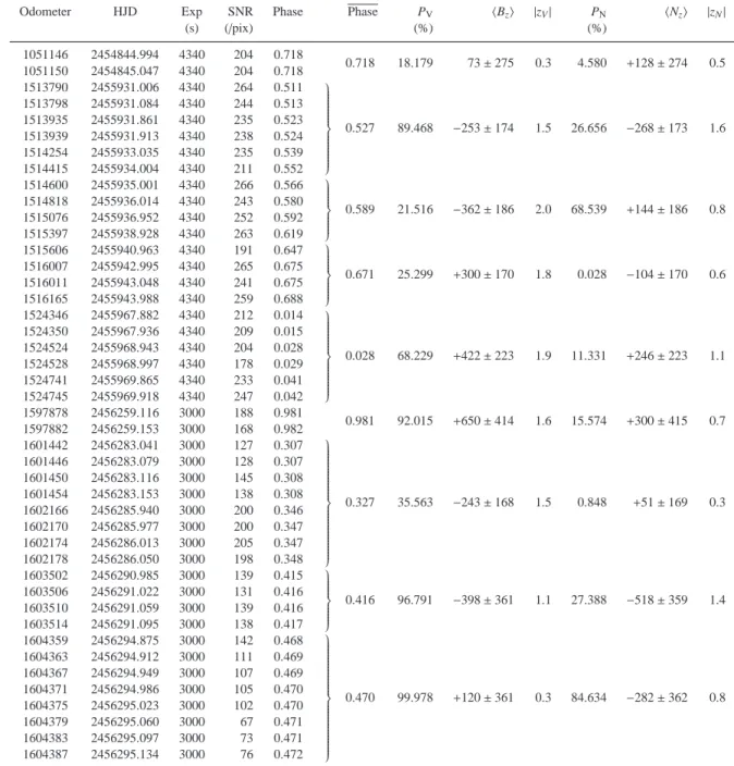
Table 3. Log of ESPaDOnS spectropolarimetric observations. Columns indicate CFHT archive unique identifier, heliocentric Julian Date, exposure duration,

signal-to-noise ratio per 1.8 km/s pixel, phase according to Eq. (1), mean phase of indicated binned spectra, Stokes V detection probability, longitudinal magnetic field and longitudinal field significance, diagnostic null detection probability, longitudinal magnetic field and longitudinal field significance.

Odometer HJD Exp SNR Phase Phase PV hBzi |zV| PN hNzi |zN|

(s) (/pix) (%) (%) 1051146 2454844.994 4340 204 0.718 1051150 2454845.047 4340 204 0.718 0.718 18.179 73 ± 275 0.3 4.580 +128 ± 274 0.5 1513790 2455931.006 4340 264 0.511 1513798 2455931.084 4340 244 0.513 1513935 2455931.861 4340 235 0.523 1513939 2455931.913 4340 238 0.524 1514254 2455933.035 4340 235 0.539 1514415 2455934.004 4340 211 0.552                          0.527 89.468 −253 ± 174 1.5 26.656 −268 ± 173 1.6 1514600 2455935.001 4340 266 0.566 1514818 2455936.014 4340 243 0.580 1515076 2455936.952 4340 252 0.592 1515397 2455938.928 4340 263 0.619                0.589 21.516 −362 ± 186 2.0 68.539 +144 ± 186 0.8 1515606 2455940.963 4340 191 0.647 1516007 2455942.995 4340 265 0.675 1516011 2455943.048 4340 241 0.675 1516165 2455943.988 4340 259 0.688                0.671 25.299 +300 ± 170 1.8 0.028 −104 ± 170 0.6 1524346 2455967.882 4340 212 0.014 1524350 2455967.936 4340 209 0.015 1524524 2455968.943 4340 204 0.028 1524528 2455968.997 4340 178 0.029 1524741 2455969.865 4340 233 0.041 1524745 2455969.918 4340 247 0.042                          0.028 68.229 +422 ± 223 1.9 11.331 +246 ± 223 1.1 1597878 2456259.116 3000 188 0.981 1597882 2456259.153 3000 168 0.982 0.981 92.015 +650 ± 414 1.6 15.574 +300 ± 415 0.7 1601442 2456283.041 3000 127 0.307 1601446 2456283.079 3000 128 0.307 1601450 2456283.116 3000 145 0.308 1601454 2456283.153 3000 138 0.308 1602166 2456285.940 3000 200 0.346 1602170 2456285.977 3000 200 0.347 1602174 2456286.013 3000 205 0.347 1602178 2456286.050 3000 198 0.348                                      0.327 35.563 −243 ± 168 1.5 0.848 +51 ± 169 0.3 1603502 2456290.985 3000 139 0.415 1603506 2456291.022 3000 131 0.416 1603510 2456291.059 3000 139 0.416 1603514 2456291.095 3000 138 0.417                0.416 96.791 −398 ± 361 1.1 27.388 −518 ± 359 1.4 1604359 2456294.875 3000 142 0.468 1604363 2456294.912 3000 111 0.469 1604367 2456294.949 3000 107 0.469 1604371 2456294.986 3000 105 0.470 1604375 2456295.023 3000 102 0.470 1604379 2456295.060 3000 67 0.471 1604383 2456295.097 3000 73 0.471 1604387 2456295.134 3000 76 0.472                                      0.470 99.978 +120 ± 361 0.3 84.634 −282 ± 362 0.8

are variable but are not the main gravity diagnostics so that our log g estimate is safe. We found that log g = 4.0±0.1 provided the best fit. In absence of strong constraint on the distance of

CPD −28◦_{2561, we decided to adopt a luminosity of 10}5.35±0.15_L

⊙.

This value is intermediate between that of an O6.5 dwarf and giant (Martins, Schaerer & Hillier 2005), and similar to that of the Of?p star HD 191612 (Howarth et al. 2007). The corresponding radius

is thus 12.9±3.0 R⊙. The best fit of the spectrum with maximum

He i 4471 absorption is shown in Fig. 1.

The evolutionary mass, determined from the position in the HR diagram and interpolation between the tracks of Meynet &

Maeder (2005), is 35±6 M⊙. The spectroscopic mass, obtained

from the surface gravity and the radius, is 61±33 M⊙. The mass

estimates are consistent within the error bars, which remain large because of the uncertainties on the distance (and thus on the lumi-nosity). We also note that the evolutionary tracks adopted here do not include the effects of a strong, large-scale stellar magnetic field. The shape of the photospheric lines could be reproduced with different combinations of rotational velocities and macrotur-bulence. In the extreme cases, a macroturbulent isotropic

veloc-ity of 40 km s−1 _{and a negligible rotational velocity, or no}

macro-turbulence and v sin i = 80 km s−1_{, correctly reproduce the shape}

of the photospheric lines. Using C iii and N iii lines as indicators (C iii λ4070 and N iii λ4505–4515 being the main diagnostics),

we estimated the nitrogen and carbon content to be N/H<5.0×10−5

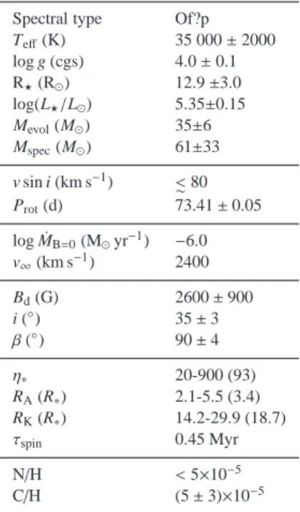
com-Table 4. Summary of physical, wind and magnetic properties of

CPD −28◦_{2561. Apart from the luminosity L/L}

⊙(which was adopted), all

parameters are derived in this paper. The mass-loss rate corresponds to the CMFGEN radiatively-driven rate required to reasonably reproduce the Hα profile; this value is only indicative, since the spherical symmetry assumed by CMFGEN is clearly broken in the case of CPD −28◦ _{2561. The wind}

magnetic confinement parameter η_∗, the rotation parameter W and the char-acteristic spin down time τspinare defined and described in Sect. 7. Values in brackets for η_∗, RAand RKcorrespond to the best-fit parameters.

Spectral type Of?p Teff(K) 35 000 ± 2000 log g (cgs) 4.0 ± 0.1 R⋆(R⊙) 12.9 ±3.0 log(L⋆/L⊙) 5.35±0.15 Mevol(M⊙) 35±6 Mspec(M⊙) 61±33 v sin i (km s−1₎ ∼ <80 Prot(d) 73.41 ± 0.05 log ˙MB=0(M⊙yr−1) −6.0 v_∞(km s−1_{) 2400} Bd(G) 2600 ± 900 i (◦_{) 35 ± 3} β(◦_{) 90 ± 4} η_∗ 20-900 (93) RA(R∗) 2.1-5.5 (3.4) RK(R∗) 14.2-29.9 (18.7) τspin 0.45 Myr N/H <5×10−5 C/H (5 ± 3)×10−5

Figure 1. Best fit CMFGEN model (red) of the observed ESPaDOnS

spectrum (black, phase 0.72, average of spectra #s 1051146/50) for CPD −28◦2561.

Figure 2. Binned ASAS photometry phased with the spectroscopic

ephemeris given by Eq. (1). Only a marginal variation is detected.

pared to the Sun, which seems consistent with the location of the star in the outer part of the disk, beyond the solar circle. The car-bon to nitrogen ratio is consistent with little enrichment: N/C<1.0, compared to 0.25 for the sun (Grevesse et al. 2010). There is no evidence for strong He enrichment. Hence the abundances of

CPD −28◦_{2561 have barely been affected by chemical processing}

occurring inside the star.

Finally, we adopted a wind terminal velocity of 2400 km s−1_,

and a velocity field slope β=1.0. These values are typical of O

dwarfs/giants. We found that a mass loss rate of 10−6_M

⊙yr−1leads

to a density ρ = ˙MB=0/(4πr2v) able to correctly reproduce the shape

of Hα in the spectrum showing the weakest nebular contamination.

We caution that this value of ˙M should not be blindly interpreted as

the true mass loss rate of this magnetic star’s outflow. As discussed

in detail in Sect. 7, the circumstellar structure of CPD −28◦_{2561 is}

expected to be highly aspherical and dominated by infalling mate-rial. MHD models by ud-Doula et al. (2008) show that for a star like

CPD −28◦_{2561, the true rate of mass lost from the star into}

inter-stellar space (i.e. from the top of the magnetosphere) is reduced by a factor of about 5, i.e. ∼ 80% of the material leaving the surface actually falls back upon the star. Hence the true mass loss rate is

most likely significantly lower than 10−6_M

⊙yr−1. Rather, the

CM-FGEN ˙MB=0should be viewed as a parameter giving a first rough

estimate of the expected circumstellar density (see further Sect. 7).

4 SPECTRAL VARIABILITY AND PERIOD

Many lines in the spectrum of CPD −28◦ _{2561 show significant}

variability.

Following a similar analysis as applied by the MiMeS col-laboration to other magnetic O-type stars (e.g. Grunhut et al. 2012; Wade et al. 2012a), we first characterise the line variability using the equivalent width (EW). Before measuring the EW, each spectral line was locally re-normalised using the surrounding continuum, and the EWs were computed by numerically integrating over the line profile. The 1σ uncertainties were calculated by propagating

0 20 40 60 80 100 Period (d) 0 500 1000 1500 2000 Power

Figure 3. Periodogram obtained from the Hα EW (solid black) and He ii

λ4686 EW (solid red) measurements. A clear and unique signal at 36.7 d is detected.

the individual pixel uncertainties in quadrature. Precomputed pixel error bars were only available for the ESPaDOnS and HARPS spec-tra, which required us to assign a single uncertainty to each pixel for the other spectra that was inferred from the RMS scatter of the Stokes I flux in the continuum regions around each spectral line.

A period search was performed on the EW measurements from all spectra using the Lomb-Scargle technique (Press et al. 1992) and an extension of this technique to higher harmonics (Schwarzenberg-Czerny 1996). In this approach, a harmonic

func-tion with free parameters a1,a2,a0and P (the latter being the

pe-riod) corresponding to the form a1sin(ωt) + a2cos(ωt) + a0, where

ω = 2π/P, is fit to the data. Adding the first harmonic leads

to the introduction of additional terms of the form a3sin(2ωt) +

a4cos(2ωt). The resulting periodograms are defined as the power

4

P

i=1

a2

i versus period P.

The periodograms from the strongly variable lines (such as Hα, Hβ, He i λ5876 and He ii λ4686) show significant power at

∼36.7 d. When phased with this period, the EW variations show

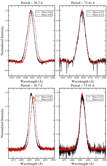
clear sinusoidal variations. However, the sinusoidal variations of the He i λ5876 measurements show considerably more scatter than the other lines. Furthermore, a comparison of spectra obtained at different epochs, but at similar phases according to the ∼36.7 d pe-riod, show important differences. These include a systematic veloc-ity offset, a difference in peak emission flux, and opposite skew, of the emission line profiles. This effect is particularly striking for Hα and He ii λ4686, and is illustrated in Fig. 4. Lines in the spectrum

of CPD −28◦_{2561 that are primarily in absorption are much more}

weakly variable; they are therefore poor probes of the wind vari-ability reflected in the emission lines. Nevertheless, the behaviour of lines that are formed deeper in the photosphere (e.g. He ii λ4542, C iv λλ5801, 5811) are indicative of a stable photospheric spec-trum that is not plausibly responsible for the phenomenon discussed above.

The detailed explanation is no different then the implementa-tion used in fsrch:

We therefore carried out a new period search including the contributions from the first harmonic - by including additional har-monics we change not only the relative power in each peak, but also the precise location of the peaks. The resulting periodograms showed two clear peaks, one consistent with the previous

peri-6550 6555 6560 6565 6570 6575 6580 Wavelength (Å) 0.9 1 1.1 1.2 1.3 1.4 1.5 Normalised Intensity Phase 0.04 Phase 0.05 Period = 36.7 d 6550 6555 6560 6565 6570 6575 6580 Wavelength (Å) 0.9 1 1.1 1.2 1.3 1.4 1.5 Phase 0.47 Phase 0.51 Period = 73.41 d 4675 4680 4685 4690 4695 4700 Wavelength (Å) 1 1.1 1.2 1.3 1.4 Normalised Intensity Phase 0.04 Phase 0.05 Period = 36.7 d 4675 4680 4685 4690 4695 4700 Wavelength (Å) 1 1.1 1.2 1.3 1.4 Phase 0.47 Phase 0.51 Period = 73.41 d

Figure 4. Comparison of Hα and He ii λ4686 profiles obtained at similar

phases, but at different epochs. Left - Assuming a period of 36.7 d, profile shapes at similar phases do not agree. Right - Assuming a period of 73.4 d, profile shapes at similar phases agree well. As discussed in the text, we identify the P = 73.41 ± 0.05 as the rotation period based on the better agreement of the profiles at all phases.

odogram at ∼36.7 d and a new peak at 73.41±0.05 d, twice the previously identified period. When phased with this longer period, the EW variations continue to phase coherently. However, this new phasing achieves a much better agreement between the line profile shapes from spectra corresponding to similar phases, but obtained at different epochs. We therefore conclude that a period of 74.41 d provides a much better solution to the phase

variabil-ity of CPD −28◦_{2561, and we adopt this period as the stellar}

ro-tation period within the context of a magnetically-confined wind and the oblique rotator model (Stibbs 1950; Babel & Montmerle 1997; Wade et al. 2011). Adopting maximum Hα emission (mini-mum EW) as the reference date we derive the following ephemeris:

HJDmax_{emis= 2454645.49(05) + 73.41(05) · E,} (1)

where the uncertainties (1σ limits) in the last digits are indicated in brackets. The uncertainties represent the formal 1σ uncertainty

computed from the χ2_{statistic corresponding to second-order}

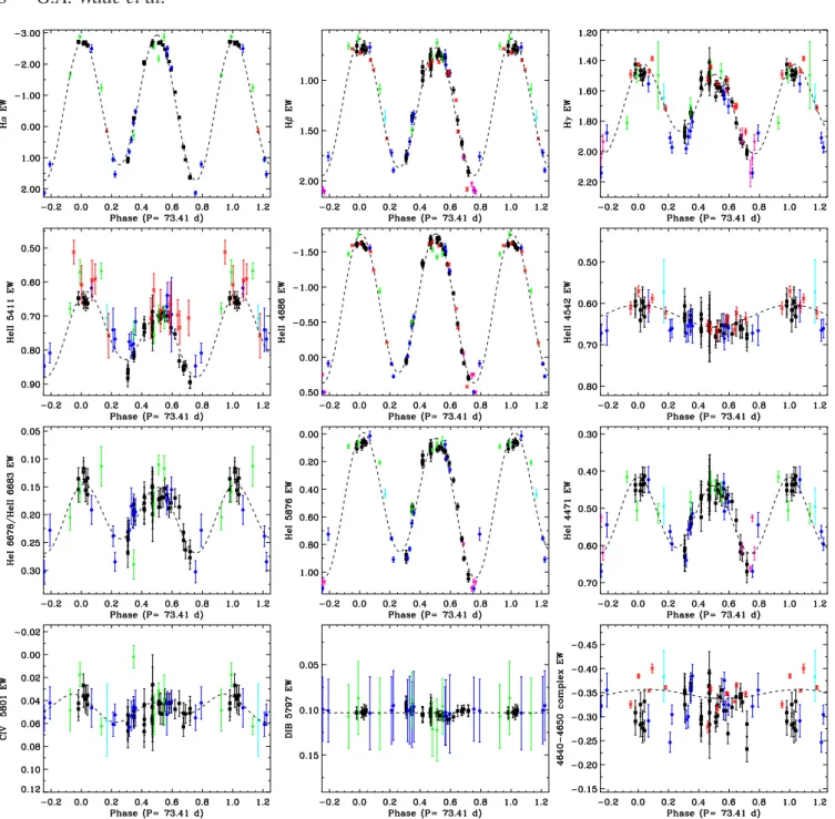
har-monic fits carried out on the EW variations for periods near 73 d. The phased EW measurements are illustrated in Fig. 5. The measurements obtained from the various spectral datasets agree reasonably well. Examination of Fig 5 shows that most lines with

significant variability exhibit double-wave variations. Hα shows the most significant variability with a peak-to-peak EW variation of ∼5 Å. Maximum emission occurs at phase 0 for most lines, while an-other emission peak occurs one-half of a cycle later. The value of the EW measurements of Hα and He ii λ4686 at maximum emis-sion are similar at both emisemis-sion maxima, while a higher emisemis-sion level occurs at phase 0.5 for some other lines (this is most evident in the EW curves of Hβ and He i λ5876), although there is consid-erable scatter at these phases. Unlike HD 148937, which showed clear variability in C iii λ4647 and C iv λ5811 (Wade et al. 2012a),

CPD −28◦_{2561 shows no significant variability in these lines. We}

also include EWs measured from the DIB at 5797 Å to illustrate the lack of variability of a reference line that is not formed in the environment of the star.

Hipparcos and ASAS data are also available for this star, and we used these data to attempt to detect photometric variability and confirm the derived period. Only the best quality data were kept : for Hipparcos, this means keeping only data with flag 0; for ASAS data, two filterings were used - either keeping only data with grade A (and discarding four strongly discrepant points with V > 10.1 mag) or keeping data only at 3 σ from the mean (both filtering yielded the same results). Errors amount typically

to 0.03 mag for Hp (Hipparcos), 0.2 mag for BT and VT

(Ty-cho), and 0.04 mag for V (ASAS). A χ2 _{test for constancy was}

performed on each dataset. Only Hp data were found to be

sig-nificantly variable with significance level S L < 1%. However, a Fourier period search on those data reveals only white noise, without any significant peaks (or in particular a peak at the ex-pected period of 73.41d). Furthermore, that period does not yield a significant coherent phased variation. Fourier period searches on the Tycho data yield similar conclusions. Period searches (Fourier (Gosset et al. 2001), PDM (Stellingwerf 1978), and en-tropy (Cincotta, Mendez & Nunez 1995)) on the ASAS data result in the detection of marginal signals with periods of 63.69 ± 0.13d and 73.43±0.16d. The amplitude is very small, ∼ 0.0046 mag at most. When phased with these periods, the photometry only shows marginal variations, even after binning the phased data (Fig. 2). We therefore conclude that any astrophysical variability of the pho-tometric signal is below the typical uncertainty of a few tens of mmag, and would require high-precision photometry to be securely detected.

4.1 Line profile variations

4.1.1 _{Line profiles of CPD −28}◦_{2561 at high resolution}

As discussed above, it is now established that CPD −28◦ ₂₅₆₁

is the only Of?p star known so far that has double emission-line maxima, corresponding to a geometry that presents both magnetic poles during the rotational cycle. The magnetic O stars HD 47129 (Grunhut & Wade 2013) and HD 57682 (Grunhut et al. 2012) do likewise. In the former case, the complex spectrum of this SB2 sys-tem precludes any identification of Of?p characteristics. In the latter case, its wind density is too low to produce the defining He ii, C iii, and N iii emission lines, while it does display the characteristic, variable Balmer emission profiles (first noted in a single Hα obser-vation by Walborn (1980). Thus, HD 57682 does provide points of

comparison for CPD −28◦_2561.

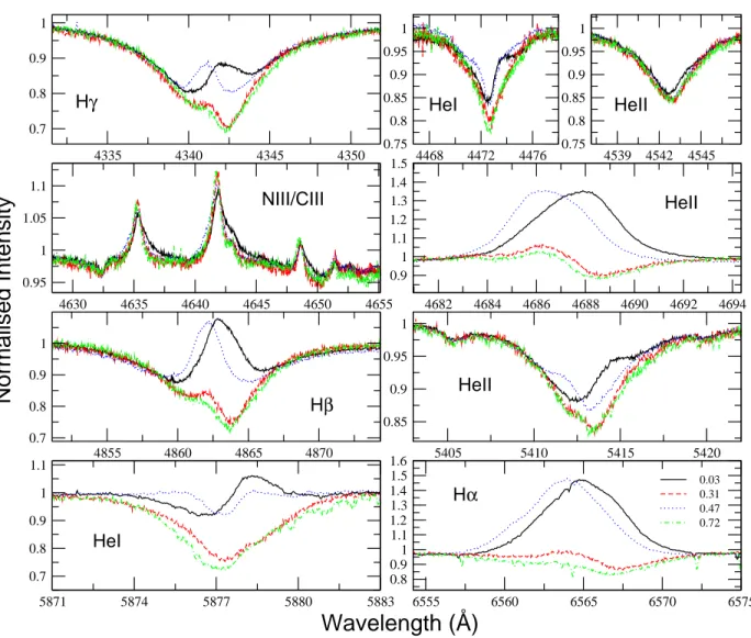
An early indication that the double-wave period of ∼ 73 d is the correct one was provided by the strikingly opposite skews of the He ii λ4686 emission peaks at phases 0 and 0.5 (Fig. 7). In ad-dition, there is a velocity offset between the two maximum phases.

Both of these effects are also seen in the Balmer emission lines to a lesser degree. Significantly, both effects are likewise seen at Hα in HD 57682. These fine morphological details undoubtedly code significant information about the complex circumstellar structures producing them.

The He ii λ4686 and Balmer profiles at the intermediate phases (i.e., at or near 0.25 and 0.75) are also noteworthy but display

diver-sity between the two objects. In CPD −28◦_{2561, they all have weak}

emission near the blueward edges of absorption features at both intermediate phases. As already noted, HD 57682 has no λ4686 emission, but remarkably, the Hα profiles have the weak emission components shifted in opposite directions at the two intermediate phases. Again, these subtle similarities and differences are impor-tant physical clues that need to be modeled and understood.

Turning to the systematic variations of He ii λ4686 during the

CPD −28◦_{2561 cycle, some further interesting effects are evident.}

The weak emission toward the shortward sides of the intermediate-phase profiles gradually strengthens and shifts toward the line cen-tre beginning about 0.3 cycle before each maximum (which again, have opposite skews and a small velocity difference). In contrast, however, the disappearance of the maximum emission lines is re-markably abrupt, occurring within about 0.1 cycle. This behavior may be suggestive of a sharp occultation of the line-emitting re-gion.

The behaviour of the dilution-sensitive line He i λ5876 is en-tirely distinct from those of the features just described, which are either similar or opposite between phases 0.5 apart. That of λ5876 is egregiously asymmetrical (Fig. 7): at phase 0.5 it displays a weak absorption flanked by equal emission wings, whereas at phase 0.0 it has a relatively weak but well marked P Cygni profile. At phases 0.25 and 0.75 it is a strong, symmetrical absorption line.

On the other hand, He ii λ5411 is a moderate absorption line with strong wings at all phases, which at first glance appears to present velocity shifts opposite to those of the λ4686 and Balmer emission lines at the two maxima. However, on closer inspection the effect is seen to be due to wing emissions in the same sense as those of the other lines, although possibly with a larger amplitude. In contrast, C iv λλ5801, 5812 are weak absorption features with no velocity shifts, albeit with a weak P Cygni tendency at phase 0.0, i.e., in the sense of λ5876. No doubt this apparent chaos will be transformed into valuable diagnostics as our understanding of the intricate phenomenology advances.

Finally, the relative behaviours of He i λ4471 and He ii λ4542 (Fig. 7) are of considerable interest, since their ratio is the primary spectral-type criterion, although classification is a heuristic exercise here because of the effects of variable circumstellar emission on the line strengths; the minimum spectrum is expected to be more closely related to the actual stellar parameters. Indeed, both lines are seen to be affected by wing emission at both maxima, albeit the He i line much more strongly. In fact, the λ4542 line has the unique characteristic that its profile at phase ∼ 0.5 is very similar to that exhibited at the quadrature phases 0.25 and 0.75. Hence it appears that this line is only affected by one of the emission maxima.

It should be noted that the He i effect is weaker than in other Of?p spectra, whereas the He ii one is unprecedented, weaker than but analogous to that in λ5411 described above. In terms of the line depths, the maximum spectral type is O7, but the He ii line has a larger equivalent width so that measurements would yield O6-O6.5. On the other hand, the minimum spectral type is a well defined O8, which again may be presumed to correspond to the stellar photosphere.

Figure 5. Rotationally phased EW measurements for selected lines in the spectrum of CPD −28◦_{2561. Least-squares sinusoidal fits are shown for those}

lines with statistically significant EW variability. In the bottom row we also show measurements of the λ5797 DIB as an example of an intrinsically non variable feature. In these figures, the ESPaDOnS measurements are black squares, the HARPS measurement is the cyan upwards facing triangle, the FEROS measurements are the blue circles, the LCO/echelle measurements are the green diamonds, the CAS measurements are the pink downward facing triangles, and the B&C measures are red crosses.

4.1.2 Dynamic spectra

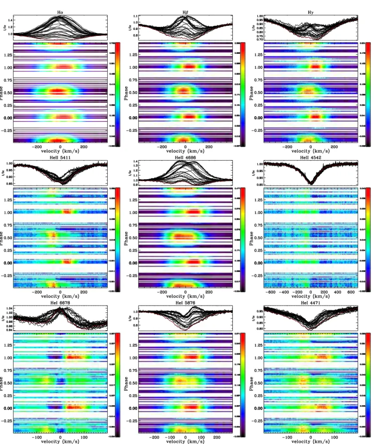
The phased line profile variations are displayed as dynamic spectra in Fig. 6. These images were constructed by subtracting the profile that presented the least overall emission in Hα (corresponding to phase ∼0.75 - obtained on HJD 2454627.467). The colour scheme was chosen to maximise the dynamic range of the variability to highlight changes relative to the minimum profile.

The dynamic spectra of the most strongly variable lines (such as the Balmer lines (Hα, Hβ, Hγ), He i λ5876 and He ii λ4686) exhibit very similar characteristics. In each case the profiles indi-cate the presence of structures that vary in intensity, from

absorp-tion to strong emission, twice per cycle. The two emission features reach similar peak intensities (as already inferred from their EW variations). The emission features of the Balmer lines are slightly asymmetric in velocity about their central peaks and are found to be broad relative to the width of the spectral line (the emission

fea-tures in Hα have a FWHM of ∼280 km s−1_{). The emission feature}

that reaches maximum emission at phase 0 appears to be offset

from the mean velocity by about -30 km s−1_{; the emission feature}

at phase 0.5 is offset by +30 km s−1_.

While the line profile variability in He i λ5876 and He ii λ4686 appears similar to the Balmer lines, there are some outstanding

Figure 6. Phased variations of selected spectral lines in the high resolution spectra, shown as dynamic spectra. Plotted is the difference between the observed

profiles and the profile obtained of HJD 2454627.467 (dashed-red, top panel), which occurred at phase ∼0.75, corresponding to minimum observed emission in Hα.

4335 4340 4345 4350 0.7 0.8 0.9 1 4468 4472 4476 0.75 0.8 0.85 0.9 0.95 1 4682 4684 4686 4688 4690 4692 4694 0.9 1 1.1 1.2 1.3 1.4 1.5

HeII

H

γ

H

β

HeI

HeII

H

α

NIII/CIII

HeI

HeII

Wavelength (Å)

Normalised Intensity

Figure 7. Selected line profiles in the spectrum of CPD −28◦_{2561 and their variability illustrated near the 4 principal phases according to the ephemeris}

derived in Sect. 4.

differences. The two emission features appear considerably more asymmetric. In fact, the emission feature occurring at phase 0.5 ap-pears to be a blend of two distinct emission peaks in both lines.

The higher intensity peak is centred around -60 km s−1_{for the He ii}

line (or −35 km s−1_{for the He i line), while the less intense peak is}

centred about 30 km s−1_{for the He ii line (or 50 km s}−1_{for the He i}

line). While the central velocities of these features differ between these two lines, their separation is similar. The emission features that appear at phases 0 and 0.5 reach similar peak intensity for the Balmer lines, whereas the intensity of the emission peak at phase 0 is about 10% stronger than the peak occurring at phase 0.5 for the He ii line and 20% stronger for the He i line.

The lines that display weaker variability exhibit a character of variability that is similar to those described for the previous lines. The He i λ6678 line shows weaker emission than the previously discussed spectral lines, but there is still evidence for an emission feature occurring twice per cycle. This feature occurs at a velocity relative to the mean velocity that is similar to the other He lines. Furthermore, the relative intensity of the redward emission feature appears considerably stronger than the blueward feature in the He i lines that display less variability (the maximum emission intensity

is about 60 percent stronger than the blueward emission feature of the λ6678 line). Some of the weakly-variable lines also show evidence of enhanced absorption (relative to the minimum profile) in a narrow region around the line core. The enhanced absorption reaches a maximum relative absorption in the core at about phase 0.5 (which corresponds to the phase of maximum emission at the blue edge of this line).

The He ii λ4542 line exhibits only weak variability. However, it stands out from essentially all other lines in the spectrum of

CPD −28◦ _{2561 due to its apparent single-wave variation, a}

phe-nomenon reflected in the line profiles examined in Sect. 4.1.1. In contrast to the double-wave variation of the other lines illustrated in Figs. 5 and 6, which show EW maxima at phases 0.0 and 0.5, the

λ4542 line appears to exhibit an EW maximum at phase 0.0, but a

minimum at phase 0.5.

5 DIAGNOSIS OF THE MAGNETIC FIELD

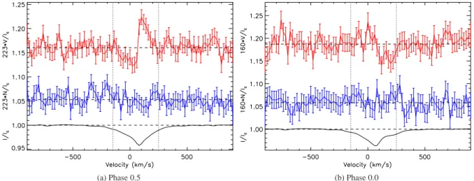
Least-Squares Deconvolution (LSD, Donati et al. 1997) was

applied to all CFHT observations using the LSD code of Kochukhov, Makaganiuk & Piskunov (2010). In their detection of

(a) Phase 0.5 (b) Phase 0.0

Figure 8. Left: LSD profile at phase 0.5, Stokes V: Definite detection (FAP=9e-7%), hBzi = −290±95 G. Diagnostic null N: ND (FAP=72%), hNzi = −2±95 G.

Right: LSD profile at phase 0.0, Stokes V: No detection (FAP=2%), hBzi = +335 ± 200 G. Diagnostic null N: ND (FAP=91%), hNzi = −71 ± 199 G.

the magnetic field of HD 191612, Donati et al. (2006) developed and applied an LSD line mask containing 12 lines. Similar masks were successfully employed by Wade et al. (2011, 2012a) in their analyses of HD 191612 and HD 148937. Given the similarity

be-tween the spectra of CPD −28◦ _{2561 and HD 191612, we began}

with this line list and adjusted the predicted line depths to best

match the depths observed in the spectrum of CPD −28◦ _{2561 at}

phases ∼ 0.25 and 0.75, when the emission is lowest. This involved adjustment of the line depths by typically ∼ 20% relative to their depths in the spectrum of HD 191612. We then used this line list to extract mean circular polarization (LSD Stokes V), mean polar-ization check (LSD N) and mean unpolarized (LSD Stokes I) pro-files from all collected spectra. All LSD propro-files were produced on

an 1800 km s−1_{spectral grid with a velocity bin of 20 km s}−1_,

us-ing a regularization parameter of 0.2 (for more information regard-ing LSD regularisation, see Kochukhov, Makaganiuk & Piskunov (2010).

Using the χ2 signal detection criteria described by

Donati et al. (1997), we evaluated the significance of the sig-nal in both the Stokes V and N LSD profiles in the velocity

range [-150, 250] km s−1_{, consistent with the observed span of the}

Stokes I profile. No significant signal was detected in any of the individual V (or N) profiles. We also computed the longitudinal magnetic field from each profile set using Eq. (1) of Wade et al. (2000a). To improve our sensitivity, we coadded the LSD profiles of spectra acquired within ±2 nights (resulting in 9 averages of 2-8 spectra; see Table 3). Given the observed variability period (Sect. 5), ±2 nights corresponds to approximately 0.05 cycles -a timesp-an during which v-ari-ability should be limited; indeed, this was verified empirically. From these profiles we obtain one

marginal detection of signal (false alarm probability FAP < 10−3₎

in the V profiles (for the coadded profile corresponding to spectral IDs 1604363-1604387), and best longitudinal field error bars of

∼ 170 G. The most significant measurement of the longitudinal

field from the coadded profiles is −362 ± 186 G (2.0σ). The individual and coadded ESPaDOnS spectra and the corresponding longitudinal fields and detection probabilities are indicated in

Table 3. The longitudinal field measured from the HARPSpol

spectrum was 280 ± 460 G.

We conclude that we fail to detect a magnetic field in

individ-ual and co-added Stokes V spectra of CPD −28◦_{2561. To proceed}

further, we note the similarity of the spectrum of CPD −28◦₂₅₆₁

to HD 191612 (and in particular its Of?p classification), and its pe-riodic variability, combined with the reported detection of a strong magnetic field by Hubrig et al. (2011, 2012), strongly suggest that

CPD −28◦_{2561 is an oblique magnetic rotator. This has been}

con-vincingly demonstrated for HD 191612 (Wade et al. 2011), and is consistent with the behaviour of other magnetic O-type stars (e.g. Wade et al. 2012b; Grunhut et al. 2012; Wade et al. 2012a).

We therefore proceeded to bin the LSD profiles according to rotational phase as computed via Eq. (1) in order to increase the signal-to-noise ratio. We note that this phase binning implicitly as-sumes an oblique magnetic rotator, i.e. that the magnetic field vari-ation proceeds according to the same period as the spectra (and other variations). We have binned the coadded LSD profiles from phases 0.307-0.619 and 0.981-0.042. From these profiles (illus-trated in Fig. 8) we obtain a definite detection of signal in the Stokes V profile (at phase ∼ 0.5) and no detection (although with twice poorer SNR) at phase ∼ 0.0, with no signal detected in the null profiles. Notwithstanding the lack of formal detection at phase 0, the Stokes V LSD profile appears to exhibit a weak signature with polarity opposite to that at phase 0.5. The phase 0.0 and 0.5

LSD profiles yield longitudinal fields of hBzi = +335 ± 200 G and

hBzi = −290 ± 95 G respectively, and corresponding null profile

fields of hNzi = −71 ± 199 G and hNzi = −2 ± 95 G. We have

also searched the average spectrum at phase ∼ 0.5 for Zeeman signatures in individual line profiles. Weak signatures, compatible with the LSD Stokes V profiles, are visible in the He i λ5876 and C iv λ5801 lines. We also note that coadding LSD profiles phased using one-half the adopted period (i.e. 36.7 d) yields no detection of the magnetic field.

From this analysis, which implicitly assumes that

CPD −28◦ _{2561 is an oblique magnetic rotator, we conclude}

that an organized magnetic field is detected in the photosphere

of CPD −28◦_{2561, with a longitudinal field with a characteristic}

strength of several hundred G, that likely changes sign.

6 STELLAR AND MAGNETIC GEOMETRY

With the inferred rotational period and derived radius (from Table

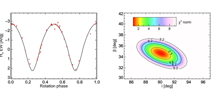
0.0 0.2 0.4 0.6 0.8 1.0 3 2 1 0 −1 −2 −3 0.0 0.2 0.4 0.6 0.8 1.0 Rotation phase 3 2 1 0 −1 −2 −3 Hα EW [Ang] 86 88 90 92 94 96 30 32 34 36 38 40 42 86 88 90 92 94 96 i [deg] 30 32 34 36 38 40 42 β [deg] 86 88 90 92 94 96 30 32 34 36 38 40 42 2.3 4.6 6.2 6.2 9.2 9.2 2 4 6 8 χ2 norm

Figure 9. MHD modelling of the Hα variation. Left - Model fit to the phased Hα EW variation. Right - χ2contour map illustrating the best fit solution of the magnetic geometry. See text for details.

in the range ve ≃ 7 − 11 km s−1_{. Since the upper limit on v sin i}

obtained in Sect. 3 (see Table 4) is much larger than this value due to the significant turbulent broadening of the line profile, we are not able to constrain the inclination of the stellar rotational axis via

comparison of veand v sin i.

Instead, we derive both the rotational and magnetic

geome-try of CPD −28◦ _{2561 from considering the rotationally}

modu-lated Hα line stemming from the star’s hypothetical circumstel-lar ”dynamical magnetosphere” (Sundqvist et al. 2012). Below the

Alfven radius RAat which the magnetic and wind energy densities

are equal, the magnetic field is strong enough to channel the

radia-tively driven wind outflow of CPD −28◦_{2561 along closed field}

lines (ud-Doula & Owocki 2002). The trapped wind plasma, chan-neled along field lines from opposite magnetic hemispheres then collides at the magnetic equator, and is pulled back to the star’s surface by gravity. This in turn leads to a statistically overdense region centered around the magnetic equator, which is also charac-terized by infalling material of quite low velocities (as compared to non-magnetic O star wind velocities). If the magnetic and rotational axes of the star are mutually inclined, an observer at earth will view this dynamical magnetosphere from different perspectives, which leads to rotationally modulated line profiles (Sundqvist et al. 2012; Grunhut et al. 2012; ud-Doula et al. 2013; Petit et al. 2013). Below we use this variability to derive constraints on the magnetic

geom-etry of CPD −28◦_2561.

We follow the procedure developed by Sundqvist et al. (2012) (see also Grunhut et al. (2012) and ud-Doula et al. (2013)) and use 100 snapshots of a 2-D radiation magnetohydrodynamic (MHD) wind simulation of a magnetic O-star, that we patch together in

azimuth to form a 3-D ”orange slice” model. The MHD

sim-ulation employed here is that computed for HD 191612 (see

Sundqvist et al. 2012) as a proxy for CPD −28◦_{2561. This is a}

rea-sonable approach because both HD 191612 and CPD −28◦ ₂₅₆₁

are slow rotators (in the sense that rotation is dynamically insignif-icant in determining the wind/magnetosphere properties), and their magnetic field strengths/confinement parameters are formally iden-tical (see Sect. 7). Hence the geometry of the plasma confinement should be similar in both cases (ud-Doula & Owocki 2002).

The tests by ud-Doula et al. (2013) show this patching

tech-nique results in a reasonably good representation of the full 3-D magnetosphere. To compute synthetic Hα spectra, we then solve the formal solution of radiative transfer in a 3-D cylindrical system for an observer viewing from angle α with respect to the magnetic axis. For magnetic obliquity β and observer inclination i we then have

cos α = sin β cos Φ sin i + cos β cos i, (2)

which gives the observer’s viewing angle as function of rotational phase Φ, thus mapping out the rotational phase variation for a

given couple of β and i3_{. We solve the formal solution only in the}

wind, assuming Hα occupation numbers and a temperature struc-ture given by a 1-D NLTE model atmosphere calculation, and us-ing an input photospheric Hα line profile as lower boundary con-dition (see Sundqvist et al. (2012) for more details). The infalling material in our selected 100 snapshots falls preferably toward one pole. This is most presumably due to a subtle numerical issue in the MHD simulations, where over a time this north-south asymmetry is canceled out (see ud-Doula & Owocki 2002). To account for the fact that in these non-rotating stars there should be no preference between the north and south magnetic pole, we here average com-puted line profiles from the same angle α as counted from the north and south magnetic poles, respectively.

The absolute level of Hα emission should further, in princi-ple, provide constraints on the rate by which the magnetosphere is fed by radiatively driven wind material (in analogy with how Hα emission from non-magnetic O-stars provides constraints on the stellar mass loss). However, as discussed in detail by Grunhut et al. (2012), adjusting the underlying model so that the level of Hα emis-sion is reproduced in the high state results in variability between the high and low states that is too small to reproduce the observa-tions. Since here we are mainly interested in obtaining constraints on the magnetic geometry from the variability itself, we thus com-pute synthetic Hα equivalent width curves that have somewhat too

3 _{Although the 2D MHD simulations of ud-Doula & Owocki (2002)} as-sumed field-aligned rotation, the slow rotation of CPD −28◦ _{2561, and}

hence the lack of any significant dynamical influence of rotation, allows us to construct 3D non-aligned structures for synthesis of Hα.

strong absolute emission and then simply shift them down so that the absolute level of emission at the extrema are fit. This then re-sults in equivalent width curves that reproduces well the variability, providing good constraints on the geometry. However, because of this shifting we are not able to simultaneously derive constraints on the mass feeding rate; this issue will be discussed in detail in a forthcoming paper.

The right panel of Fig. 9 shows the χ2 _{landscape from fitting}

the observed rotational phase variation for given sets of β and i. Because of the strong emission dependence on α, the error bars of the best fit i = 90 deg and β = 35 deg are quite small. We note, however, that simply switching the obliquity and inclination angles gives equal results, i.e. there is a second ”best-fit” model at i = 35 deg and β = 90 deg (that is not shown in the figure). The left panel then finally compares the best model with the observed variability as function of rotational phase.

6.1 Photometric and broadband polarization variability

A second constraint on the geometry is potentially derived from photometric and broadband (linear) polarimetric variability. We use the Monte-Carlo radiative transfer (RT) code developed by RHDT for simulating light scattering in circumstellar envelopes, first ap-plied in this context to the Of?p star HD 191612 by Wade et al. (2011). In this code, photon packets are launched from a central star and allowed to propagate through an arbitrary distribution of circumstellar matter (described by a Cartesian density grid), un-til they are scattered by free electrons. Upon scattering, a ray is peeled off from the packet toward a virtual observer, who records the packet’s Stokes parameters appropriately attenuated by any in-tervening material (see Yusef-Zadeh, Morris & White 1984, for a discussion of this peel-off technique). A new propagation direction is then chosen based on the dipole phase function (Chandrasekhar 1960), and the packet’s Stokes parameters are updated to reflect the linear polarization introduced by the scattering process. The prop-agation is then resumed until, after possible further scatterings, the packet eventually escapes from the system or is reabsorbed by the star.

We employ the circumstellar density model developed for HD 191612, and compute lightcurves for the two geometries derived from the orange-slice MHD modelling. In Fig. 10 we compare the observed ASAS V-band photometric variation with the predictions of the Monte Carlo RT code. Unfortunately, the available photome-try is not sufficiently precise to allow us to obtain meaningful con-straints on the geometry. Nevertheless, the predictions demonstrate that the existing photometry is at the threshold of being able to de-tect the predicted variation. High-precision photometry and broad-band polarimetry would provide an additional constraint on the ge-ometry, and in particular the polarimetric variation would enable the determination of the individual values of the angles i and β.

6.2 Longitudinal magnetic field variation

To infer the strength of the magnetic field, and to test its compati-bility the derived geometry, we model the longitudinal field

vari-ation of CPD −28◦ _{2561 as a function of rotational phase. We}

used the coadded profiles discussed in Sect. 5 and reported in

Ta-ble 3, phased according to Eq. (1). This phase variation hBzi(φ)

of the longitudinal field is illustrated in Fig. 11 (upper frame).

A fit by Least-Squares of a cosine curve of the form hBzi(φ) =

B0+ B1cos(2π(φ − φ0)) to the data yields a reduced χ2 of 0.84,

with parameters B0 _{= +115 ± 55 G, B}1 = 450 ± 100 G and

φ0= 0.18 ± 0.15.

Therefore, according to Least Squares, the variation of the

field is detected at 4.5σ confidence. The reduced χ2 _{of the data}

relative to the straight line hBzi(φ) = 0 (the hypothesis of a null

field) is 2.3. These results indicate that the variation is significant at about 97% confidence, and that the null hypothesis can be re-jected as an acceptable representation of the data at similar confi-dence. The longitudinal field measured from the null profiles (lower

frame of Fig. 11) yields similar reduced χ2_{for both the cosine and}

straight-line fits, and indicates no significant variation.

Adopting i = 35◦ _{and β = 90}◦ _{from the modelling of the}

Hα EW, we have fit the phase-binned longitudinal field measure-ments with a synthetic longitudinal field variation with fixed phase of maximum (phase 0.5) and variable polar field strength Bd. The

best-fit model (according to the χ2 _{statistic) is characterised by}

Bd≃ 2.6 kG. The extrema of the best-fit dipole model are slightly

offset from the best-fit sinusoid in mean longitudinal field strength (by about 100 G) and in phase (by about 0.07 cycles). These offsets are well within the uncertainties of the observed variation. Taking them into account, we estimate an uncertainty on the derived dipole strength of ±900 G.

If we fix only the inclination and allow both β and Bdto vary,

a direct fit to the longitudinal field variation yields best-fit values of

β =78+10

−8 ◦and Bd= 2.7 ± 1.1 kG. These values are in good

agree-ment with those derived from the fit with fixed geometry derived above.

In Fig. 11 we also show the longitudinal field measurements of Hubrig et al. (2011, 2013) obtained from ’all’ lines. Those measure-ments, which have formal errors that are substantially more precise than our own, are in good agreement with both the best-fit synthetic dipole and the best sinusoidal fit. It is notable that 3 of the measure-ments of Hubrig et al. were acquired at essentially the same phase,

which corresponds to crossover (i.e. hBzi ≃ 0).

6.3 Modeling the Stokes V profiles

We also modelled the magnetic field geometry using the LSD Stokes V profiles. We compared the mean LSD profiles for phases 0.0, 0.5 and 0.75 to a grid of synthetic Stokes V profiles using the method of Petit & Wade (2012). For this modelling we used LSD profiles extracted using a metallic line mask, as described by Wade et al. (2012a).

The emergent intensity at each point on the stellar surface is calculated using the weak-field approximation for a Milne-Eddington atmosphere model. In this model, the source function is

linear in optical depth such that S (τc) = S0[1+βτc]. We use β = 1.5,

Voigt-shaped line profiles with a damping constant a = 10−3_{and a}

thermal speed vth = 5 km s−1_{. The line-to-continuum opacity}

ra-tio κ is chosen to fit the intensity LSD profile. The synthetic flux profiles are then obtained by numerically integrating the emergent intensities over the projected stellar disk. The projected rotational

velocity is set to v sin i = 9 km s−1_{. We applied isotropic Gaussian}

macroturbulence4_{compatible with that determined in Sect. 3.}

We assume a simple centred dipolar field, parametrized by the

dipole field strength Bd, the rotation axis inclination i with respect

to the line of sight, the positive magnetic axis obliquity β and the ro-tational phase ϕ. Assuming that only ϕ may change between differ-ent observations of the star, the goodness-of-fit of a given

rotation-4 _{of the form e}−v2_/v2

0.0 0.2 0.4 0.6 0.8 1.0 Phase 9.90 9.92 9.94 9.96 9.98 10.00 10.02 10.04 V i= 35◦ i= 90◦ ASAS 0.0 0.2 0.4 0.6 0.8 1.0 Phase −0.4 −0.2 0.0 0.2 0.4 Q / I (% ) 0.0 0.2 0.4 0.6 0.8 1.0 Phase −0.4 −0.2 0.0 0.2 0.4 U / I (% )

Figure 10. Predicted light curve and broadband polarization variations of CPD −28◦_{2561. Variations are shown for two models: (i = 35}◦_{, β =90}◦_{), and}

(i = 90◦_{, β =35}◦_{). Whereas both models produce identical light curves, their polarization variations are clearly distinct.}

Figure 11. Top panel: Longitudinal field versus phase. Dashed line -

best-fit sinusoid. Solid line - Dipole model (fixed phase and geometry, polar strength Bd= 2.6 kG). Diamonds represent ESPaDOnS measurements from

the current study. The cross is the HARPSpol measurement. The triangles are measurements from Hubrig et al. (2011, 2013). Bottom panel: Null field versus phase. All measurements are phased according to Eq. (1).

independent (Bd, i, β) magnetic configuration can be computed to

determine configurations that provide good posterior probabilities for all the observed Stokes V profiles in a Bayesian statistic frame-work. In order to stay general, we do not at this point constrain

Table 5. Odds ratios derived from the analysis of Stokes V profiles.

Phase log(M0/M1) V log(M0/M1) N

0.00 -0.91 0.09

0.50 -7.43 0.24

0.75 -0.34 0.06

Combined -9.06 0.25

the rotational phases of the observations nor the inclination of the rotational axis.

The Bayesian prior for the inclination is described by a ran-dom orientation [p(i) = sin(i) di], the prior for the dipolar field strength has a modified Jeffreys shape to avoid a singularity at

Bd= 0 G, and the obliquity and the phases have flat priors.

To assess the presence of a dipole-like signal in our observa-tions, we compute the odds ratio of the dipole model (M1) with the null model (M0; no magnetic field implying Stokes V = 0). We also perform the same analysis on the null profiles. The results are displayed in Table 5. Taking into account all the observations si-multaneously, the odds ratio is in favour of the magnetic model by 9 orders of magnitude. For the null profiles, the combined odds

ra-tio is 2:1 in favour of the null model. Note that as the case Bd= 0 G

is included in the magnetic model, in the latter case the difference between the two models, which can equally well reproduce a signal consisting of only pure noise, is expected to be dominated by the ratio of priors in this case, i.e. the Occam factor that penalizes the magnetic model for its extra complexity.

Figure 12 shows the posterior probability density function for each model parameters. The 68.3, 95.4, 99.0, and 99.7 percent re-gions, tabulated in Table 6, are illustrated in dark to pale shades, respectively. At 95.4% confidence, the polar strength of the dipole

magnetic field of CPD −28◦ _{2561 is found to be in the range}

1.9 6 Bd 6 _{4.5 kG. This is in good agreement with the dipole}

strengths derived from the longitudinal field variation.

7 MAGNETOSPHERE

As presented by ud-Doula & Owocki (2002), the global compe-tition between the magnetic field and stellar wind can be

char-Table 6. Credible regions derived from the Bayesian analysis of Stokes V

profiles.

Credible Range in gauss region V 99.7 1754 - 5000 99.0 1841 - 4947 94.5 1891 - 4509 68.3 2137 - 3307 N 99.7 0 - 3835 99.0 0 - 2767 95.4 0 - 1508 68.3 0 - 425

Figure 12. Magnetic field polar strength (upper frame) and geometry (i, β)

(lower frame) constraints derived from of modelling of Stokes V profiles.

acterized by the so-called wind magnetic confinement parameter

η⋆ ≡ B2eqR

2

⋆/ ˙MB=0v∞, which depends on the star’s equatorial field

strength (Beq), stellar radius (R⋆), and wind momentum ( ˙MB=0v∞)

the star would have in absence of the magnetic field. For a dipolar

field, one can identify an Alfv´en radius RA ≃ η1/4⋆ R⋆,

represent-ing the extent of strong magnetic confinement. Above RA, the wind

dominates and stretches open all field lines. But below RA, the wind

material is trapped by closed field line loops, and in the absence of

significant stellar rotation is pulled by gravity back onto the star within a dynamical (free-fall) time-scale.

To estimate the Alfv´en radius of the magnetosphere of

CPD −28◦_{2561, we use the stellar parameters given in Table 4.}

The stellar parameter with the largest uncertainty is the wind

momentum. Fig. 13 therefore illustrates the variation of RA with

one order of magnitude variation in mass-loss rate (corresponding to a generous estimate of the uncertainty). One can see how this uncertainty is mitigated by the 1/4 power dependence of the wind momentum in the definition of the Alfven radius. The grey shaded

areas represent intervals of stellar radius uncertainty (±3 R⊙) and

of dipole field strength (2.1, 2.6, 3.3 kG, reflecting the 68.3% Bayesian credible region) meant to minimize and maximize the Alfven radius.

We therefore expect the Alfven radius to be of the order of 3 stellar radii, and certainly no more than 5 stellar radii.

In the presence of significant stellar rotation, centrifugal forces can support any trapped material above the Kepler co-rotation

radius RK ≡ (GM/ω2₎1/3_{. This requires that the magnetic}

con-finement extend beyond this Kepler radius, in which case ma-terial can accumulate to form a centrifugal magnetosphere (e.g. Townsend, Owocki & Groote 2005).

In the case of CPD −28◦_{2561, the slow rotation puts the}

Ke-pler radius much farther out than the Alfven radius (∼ 18 R⋆) and

no long-term accumulation of wind plasma is expected, as illus-trated by the red curve in Figure 13 (the red shaded area represents

±3 R⊙and a range of mass from 30 to 60 M⊙). In such a

dynami-cal magnetosphere configuration, transient suspension of

circum-stellar material results in a statistical global over-density in the closed loops. For O-type stars with sufficient mass-loss rates, the resulting dynamical magnetosphere can therefore exhibit strong emission in Balmer recombination lines (Sundqvist et al. 2012; Petit et al. 2013). This conclusion supports the MHD modelling employed to determine the stellar geometry in Sect. 6. We note that due to infalling wind material (which may be reflected in the P Cyg-like profile of He ii λ4686 at some phases), the global mass-loss rate of a star exhibiting such a dynamical magneto-sphere is significantly reduced. According to the scaling relations of Ud-Doula, Owocki & Townsend (2008) (their eqn. 10 and 23),

for an estimated rA ≈ 3Rstar, ˙M/ ˙MB=0 ≈ 0.2, i.e. the global

mass-loss rate is reduced by approximately a factor of 5 due to wind plasma falling back upon the star.

The characteristic magnetic braking time can be estimated us-ing equation 25 of ud-Doula, Owocki & Townsend (2009). Usus-ing the nominal wind parameters in Table 4 and k ∼ 0.1 (Claret 2004), we obtain a spin-down timescale of 0.45 Myr. However as noted by Petit et al. (2013), the square-root dependence of this quantity on the wind momentum renders spin-down estimates valid only to a factor of a few.

8 DISCUSSION AND CONCLUSIONS

In this paper we have performed a first thorough analysis of the variability, geometry, magnetic field and wind confinement of the

Of?p star CPD −28◦_{2561. Using more than 75 new medium and}

high resolution spectra, we determined the equivalent width varia-tions and examined the dynamic spectra of photospheric and wind-sensitive spectral lines, deriving a rotational period of 73.41 d. We confirmed the detection of an organized magnetic field via Zeeman signatures in LSD Stokes V profiles. The phased longitudinal field data exhibit a weak sinusoidal variation, with maximum of about