Robustness of Planar Shape Descriptors of Particles E. Pirard1, G. Dislaire1
1Université de Liège, GeomaC, Mineral Resources and Geo-imaging Lab Sart Tilman B52, 4000 Liège, Belgium,
E-mail : eric.pirard@ulg.ac.be 1. Abstract
This paper explores the estimation error of size and shape parameters computed from binary digital images of individual particles. The influence of sampling density (magnification), translation and rotation of the discrete grid is studied using simulated images of geometric and natural particles. These results are intended to serve as a basis for selecting the most adequate size and shape estimators in image analysis. They also warn users against abusive comparison of shape parameters obtained on particlesof different size (or at different magnification).
2. Introduction
The literature on shape analysis is extremely extensive, particularly in the field of geology and sedimentology, where regular review publications help to keep trace of some major contributions. Despite the sophistication of multiscale analysis techniques making use of Fourier spectrum analysis (Ehrlich and Weinberg, 1970), Fractal dimensions (Kaye, 1995) or Mathematical Morphology (Serra, 1982) the practical results gained so far are still limited. This disappointment is probably due to the fact that the quest for the supreme morphometric method is desviating many researchers from the necessity to compare, validate and select the methods satisfying basic quality criteria. These have been already defined by Exner (1980) : Independency; Robustness; Sensitivity; Accessibility; Additivity; Relevance.
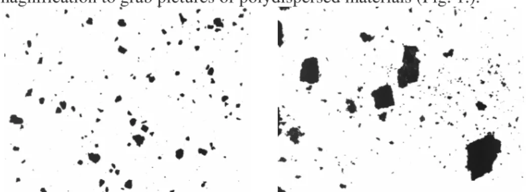
It is the objective of this paper to compare the robustness of the most popular global shape parameters with respect to the density, translation and rotation of the sampling grid. The practical implications of the results are essential in that they indicate whether it is acceptable to compare measurements performed using different algorithms (thus different commercial image analyzers) and to which extent it is allowable to compare shape parameters obtained at different magnifications as well as on particles of variable size pictured at equal magnification. This last problem is central because most systems work at fixed magnification to grab pictures of polydispersed materials (Fig. 1.).
3. Test shapes and image simulation methods.
The robustness of shape parameters can be tested using analytical, experimental or simulation techniques. Analytical techniques are extremely powerful because they can be solved to compute the Best Unbiased Estimator, but they can only be developed for simple geometric shapes (disk, rectangle,…). Experimental imaging consists in taking pictures at different magnifications of objects lying on a turntable. Apart from being time consuming, this method can only explore a limited set of magnifications determined by the available optics and suffers from any additional variation that can affect the optical system (optical abberation, heating up of the camera, change in light intensity, etc.). Finally simulation is an idealized context in which the estimation error is on the lowest side. But, it allows to explore a large number of situations and to analyze a wide range of shapes without departing too much from reality.
In this study, both geometric shapes and real shapes have been studied (Fig. 2). The shapes are represented as black pixels sets (level 0) on a white background (level 255). In order to simulate the optics a Gaussian interpolation function is applied and thresholded at level 128 to determine the border forming pixels for each position of the grid.
Subpixel translation of the grid has been explored using steps of x= y=0.05 (5% of the interpixel distance) in the interval of coordinates [0,0] and [0.5,0.5]. Rotation of the grid has been explored using steps of =7.5° in the interval between 0° and 45°.
A
B
Fig. 2. A. Set of real particles (diamond, sand, rutile, glass bead) used for testing in addition to ellipses and disks. B. Sand particle sampled at 9000, 2300, 600, 140 pixels and rotated 30° at 600.
4. Area, Perimeter and Aspect Ratio Estimators.
Basic stereology (Stoyan, 1995) demonstrates that the best unbiased area estimator is obtained by counting the pixels of a systematic grid hitting the object (Pi) and multiplying by their area of influence (dA):
= i i
dA P
A . (1)
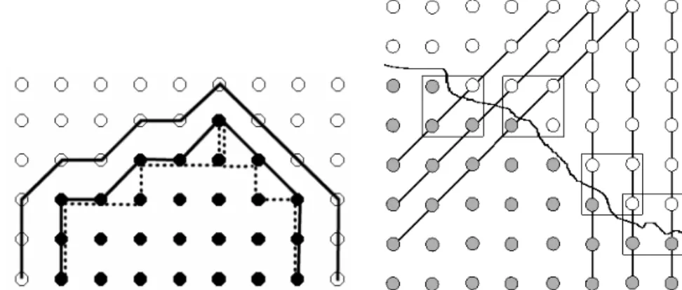
Another well known result is the perimeter estimator of a disk based on the number of intercepts (I ) formed by a series of parallel lines with spacing d exploring N directions from 0 to (Fig. 3). This gives the so-called Cauchy-Crofton formula :
d I N U . 0 = = π α α
π
(2)The vast majority of image analysis systems ignore this formula and use either a simple count of the border pixels (4c inner perimeter) or a polygonal approximation linking these border pixels with an eight-connected chain (8c inner perimeter), not to say that some
might use similar definitions applied to the background border pixels (outer perimeter) (Fig.3). Dorst & Smeulders (1987) suggested a Best Linear Unbiased Estimator for the length of a circular arc from its 8c polygonal approximation.
Fig. 3. A. Based on the object ( ) and background ( ) pixels it is possible to consider different perimetric representations : inner 4c (dotted line), inner 8c or outer 8c (continuous line).
B. Some intercept configurations in both the 45° and 90° orientations.
The most common shape parameter is called circularity (shape factor, isoperimetric deficit, etc.). It is a simple ratio obtained from the previous estimators :
2 . . 4 U A F =
π
(3)It is derived from Euclidean geometry and is used to express the departure from a perfect disk. However, it is clear from many practical examples (fig.4) that it confuses both a notion of elongation and roughness.
Fig. 4. These particles are clearly different in terms of roundness or elongation. A circularity measure will not be able to distinguish a from b (F=70%) or c from d (F=61%).
The elongation of a particle is the ratio between its largest and its smallest diameter in a 2D projection. A common estimator of the diameter of the particle is the Feret diameter, (F ) which is the length of its projection onto a segment making an angle of with the reference axis. From a series of projections a minimum and a maximum can be derived to compute an aspect ratio (Russ, 1990): ELF. Inertia moments are a popular way of fitting an equivalent ellipse to any given shape. The axial ratio of this ellipse is another possible estimation for the elongation of the particle (Medalia, 1970): ELI
5. Data analysis Area estimation
The dispersion of the area estimator with rotation is obtained for different sampling densities ranging from about 20 pixels up to 10000 pixels per object. The estimator appears clearly unbiased above 200 pixels, whereas underestimation occurs in practice at lower resolution. For the glass bead the maximum error is only 4 % but it can be as worse as 15 % for more elongated particles (Fig. 5).
Fig. 5. Area estimation as a function of the sampling density (log scale) for two particles.
Perimeter estimation
The estimation of the perimeter of a perfect disk of radius 100 for a series of rotations and translations is given in fig. 6.A. for pixel densities ranging from 15 up to 31000 pixels. The unbiased nature of the Cauchy-Crofton estimator, even using N=4, is clear when compared to the classical 8c perimeter. Fig. 6.B. presents the same results in terms of the squared error of the perimeter estimation for different sampling densities.
A B
Fig. 6. A. Box-Whisker plots for perimeter estimates of a disk. B. Squared error on the perimeter estimate of a disk as a function of the sampling density (log scale)
The Cauchy-Crofton formula still appears to be the most unbiased estimator for a 2:1 ellipse although the variance is quite higher than for 8c polygonal estimation (Fig. 7.A.). This is confirmed for real irregular shapes such as the sand grain (Fig. 7.B.).
A B
Fig. 7. A. Box-Whisker plots for the squared error on the perimeter estimate of an ellipse as a function of sampling density (log). B. Perimeter estimations for a sand grain.
Glass Bead
25
50 75 250 500750 2500 50007500 Grid Density (Nb Pixels)
70 75 80 85 90 95 100 D iff to A ve ra ge A re a (% ) Broken Diamond 25 50 75 250 500750 2500 50007500 Grid Density (Nb Pixels)
70 75 80 85 90 95 100 D iff to A ve ra ge A re a (% )
Circularity estimation
As a ratio of the area to the squared perimeter, the bias of the circularity estimator is quite significant. Fig. 8 shows its evolution with sampling density for a perfect disk. A similar behaviour is seen with the sand grain. This clearly demonstrates that using the 8c perimeter estimator, not only is circularity never equal to unity, but it is hazardous to compare circularity factors of small (200 pixels) versus large (5000 pixels) particles. Using Crofton, the estimation is less biased, but its standard deviation is higher.
A B
Fig. 8. A. Plot of circularity estimations for a disk as a function of sampling density (log) for all possible grid translations and rotations.
B. Circularity as a function of sampling (log) and rotation for a sand grain.
Elongation estimation
Except for elliptical shapes, inertia moments will not give the exact dimensions of an object and hence its exact elongation (Fig. 9). The advantage of using inertia moments lies in the robustness of the method with respect to the orientation of the major and minor axes. Therefore, a suggested technique (Pirard, 2004) is to compute Feret dimensions from the orientations given by inertial ellipses.
A B
Fig. 9. A. Box-Whisker plots for elongation estimations of a 2:1 ellipse as a function of sampling density (log) for all grid rotations and translations.
B. Elongation as a function of sampling density (log) and rotation for a sand grain.
6. Conclusion
The precise estimation of size and shape properties of objects is essential in image analysis. The simulated results clearly indicate that it might be hazardous to compare measurements made at different scales or to compare shape parameters through the whole size range.
Experimental imaging on real and synthetic shapes have confirmed the results presented in this study. Though one must consider simulations as giving the lower bound of estimation errors, it is clear that some estimators perform better than others for the range of quasi-convex shapes explored in this work which are considered representative of many granular materials.
As a conclusion, the Cauchy-Crofton estimator should be recommended for all perimeter based measures and Feret ratios derived from the orientation of the main inertia moments should be promoted as the most robust and accurate method for aspect ratio computations.
7. References
Dorst, L., and Smeulders, A. W., 1987 : Length estimators for digitized contours. Computer Vision Graphics and Image Processing, 440, 311-333.
Ehrlich, R., and Weinberg, B., 1970 : An exact method for characterization of grain shape. J Sedimentary Petrology, 40, 205-212.
Exner, H. E., 1987 : Shape : a key problem in quantifying microstructures. Acta Stereologica, 6, 1023-1028.
Kaye, B., 1995 : Applied fractal geometry and powder technology. In Chaos, Solutions and Fractals, 6, 245-253.
Medalia, A., 1970 : Dynamic shape factors of particles. Powder Technology, 4, 117-138.
Pirard, E., 2004 : Image Measurements. In Image analysis, sediments and paleoenvironments, Developments in paleoenvironmental research. 7. Dordrecht, Kluwer.
Russ, J. C., 1990 : Computer-Assisted Microscopy. The measurement and analysis of images. New York, Plenum Press.
Serra, J., 1982 : Image analysis and mathematical morphology. New York, Academic Press. Stoyan, D., Kendall, W. S., and Mecke, J., 1995 : Stochastic Geometry and its Applications. Chichester, Wiley.