SPICES: a 1.5-m space coronagraph for spectro-polarimetric
characterization of cold exoplanets
Anne-Lise Maire
a, Anthony Boccaletti
a, Jean Schneider
b, Rapha¨
el Galicher
c, Pierre Baudoz
a,
Daphne Stam
d, Wesley Traub
e, Pierre-Olivier Lagage
f, Raffaele Gratton
g,
and the SPICES team
a
LESIA, Paris Observatory, CNRS, 5 pl. J. Janssen, 92195 Meudon, France;
bLUTh, Paris Observatory, CNRS, 5 pl. J. Janssen, 92195 Meudon, France;
c
Herzberg Institute of Astrophysics, 5071 West Saanich Road, Victoria, BC V9E 2E7, Canada;
dSRON, Sorbonnelaan 2, 3584 CA Utrecht, The Netherlands;
e
JPL, California Institute of Technology, 4800 Oak Grove Drive, Pasadena, CA 91109, USA;
fSAp, CEA Saclay, 91191 Gif-sur-Yvette, France;
g
INAF-Padova Observatory, Vicolo dell’Osservatorio 5, Padova, Italy, 35122-I
ABSTRACT
The study of the physico-chemical properties of wide-separated exoplanets (> 1 AU) is a major goal of high-contrast imaging techniques. SPICES (Spectro-Polarimetric Imaging and Characterization of Exoplanetary Systems) is a project of space coronagraph dedicated to the spectro-polarimetric analysis of gas and ice giant planets, super-Earths and circumstellar disks in visible light at a spectral resolution of about 40. After recalling the science cases of the mission, we describe the optical design and the critical subsystems of the instrument. We then discuss the SPICES performance that we derived from numerical simulations.
Keywords: high angular resolution techniques, high-contrast imaging techniques, exoplanets, integral field spectro-polarimetry
1. INTRODUCTION
The field of exoplanets in astrophysics is extremely rich and diverse. From detection to characterization, many techniques are being used or developed to address the fundamental questions about planetary formation and evolution. Some are more efficient to build statistics on the planet frequency and parameters (radial velocities,1 microlensing2) while others provide information on the composition and structure of planetary atmospheres (transits,3direct imaging4). Direct imaging is currently the only available technique for the spectral
characteri-zation of long-period planets, from a few tenths to several hundreds of astronomical units (AU). In the present decade, planet-finder instruments on 8–10-m class telescopes will analyze young and/or nearby jovian planets in near-infrared spectroscopy and visible polarimetry. In the 2020s, extremely large telescopes (E-ELT5) and
space observatories (JWST,6 SPICA7) will be sensitive to lighter and colder giant planets. Possibly, the former
will detect super-Earths but will not be able to perform spectral analyses of such faint planets in great details. Conceptual studies were carried out to consider the feasibility of large aperture coronagraphs and large baseline interferometers for the detection of Earth twins from space. These studies identified areas of technological de-velopment that need to be first addressed, which postpone the realization of Terrestrial Planet Finder missions in ∼2025–2030. Several missions, mainly small coronagraphs,8, 9 have been proposed to 1/ get colors and/or
low-resolution spectra of ice giants and super-Earths in the solar neighborhood (.20 pc) and 2/ validate the key technologies required for the realization of larger instruments for the characterization of Earth twins. SPICES (Spectro-Polarimetric Imaging and Characterization of Exoplanetary Systems) belongs to this family of projects but differs from them in several aspects. First, it will measure the spectro-polarimetric information of a planet at a spectral resolution of 40 while the others will provide colors and spectro-photometry at a resolution ≤15.8, 9 Then, since accurate spectral measurements are time demanding (from a tens of hours to a few hundred hours10),
it will focus on planetary systems previously discovered by other instruments instead of performing discovery surveys. This proposal was submitted to the ESA Cosmic Vision call for medium-class missions in 2010 by a consortium of European institutes with American and Japanese participations.11 We briefly review the science
cases of the mission in Sec. 2. Then, we describe the optical design, the pointing issues and the mission profile in Sec. 3. Finally, Section 4 illustrates the instrument performance that we derived from numerical simulations. We refer the reader to a companion paper published in these proceedings and to Maire et al.10 for a more detailed
description of the results of this last section.
2. SCIENCE CASES
The main science driver of SPICES is the study of planetary systems as a whole for the understanding of planet formation and evolution. This includes of course cold planets, which are definitely the main goal of the mission, but also planets with longer periods (>10 AU) around young stars (found by planet finders on the ground) and circumstellar disks (from protoplanetary to debris disks). SPICES also potentially offers discovery capability through surveys around bright/nearby stars. Importantly, SPICES can detect exozodiacal light, which is famously known to hamper the detection of Earth-like planets, down to a few zodis. Therefore, the census SPICES will carry out will be crucial for future space nulling interferometers.12, 13
SPICES direct imaging and spectro-polarimetry (R = 40) will give us information on: • the composition of planetary atmospheres (absorbing gases);
• the presence and character of clouds/hazes;
• the structure of planetary atmospheres (e.g. vertical distributions of gases, clouds and hazes); • the composition and structure of planetary surfaces (if present and visible through the atmosphere); • temporal variations in the composition and structure of planetary atmospheres and surfaces (e.g. due to
seasons, orbital eccentricity, chemical non equilibrium);
• the rotation rate of a planet (only for slow rotators with high-contrast surface features);
• the orientation of planetary orbits (yielding the true masse for planets detected with the radial velocity method);
• the presence of unknown exoplanets in known planetary systems;
• the properties (density, microphysical characteristics) of exozodiacal dust; • the morphology of circumstellar dust and debris disks.
In the remainder of this section, we focus on the main science cases of SPICES, namely the spectro-polarimetric analysis of cold planets and the expected number of targets.
2.1 Visible spectro-polarimetry of cold extrasolar planets
Old planets are cold, and at visible wavelengths, they shine with the starlight they reflect. SPICES will measure the polarized flux from 0.45 to 0.90 µm. The reflected planet flux is a function on its radius, its distance to the star, its distance to the observer and its albedo. The latter is dependent on the composition and structure of the planetary atmosphere and surface (if present and visible through the atmosphere), the wavelength, and the planetary phase angle (i.e. the angle star-planet-observer).
0.4 0.5 0.6 0.7 0.8 0.9 1 0 0.1 0.2 0.3 0.4 0.5 0.6 0.7 0.8 0.9 1 Wavelength, µm Albedo
Jupiters and Neptunes
CH₄ CH₄ CH₄ CH₄ CH₄ CH₄ H₂O H₂O CH₄ Na K CH₄ CH₄ H₂O H₂O K 2 AU Jupiter (green) 2 AU Neptune (cyan) 0.8 AU Jupiter (red) 0.8 AU Neptune (blue)
Figure 1. Left: Albedo spectra of model Jupiter and Neptune planets at separations of 0.8 AU (red and blue respectively) and 2 AU (green and cyan respectively). Rayleigh scattering is clearly seen for the 0.8-AU model because the atmosphere temperature is too warm for the cloud formation. The 2-AU models are cold enough to allow water to condensate into clouds, which greatly increases the amount of reflected light and the contrast between the molecular bands and the continuum. Right: Albedo spectra of Venus (yellow), the Earth with clouds (purple), the Earth without clouds and an ocean (black) and Mars (red) (Tinetti et al.17). The spectra differ strongly because of different compositions, cloud optical thicknesses and type surfaces.
2.1.1 Gas and ice giants
The left panel of Fig. 1 shows albedo spectra for models of Jupiter-like (red and green curves) and Neptune-like (blue and cyan curves) planets, for a spectral resolution of 40. Even at such a low resolution, SPICES will be able to distinguish between gas and ice giants. Indeed, the atmosphere of the Neptune-like planets contains more methane which absorbs light at all wavelengths for a separation of 0.8 AU, and especially in the methane bands for 2 AU (0.54, 0.62, 0.73, 0.79 and 0.89 µm). Measuring absorption bands at different wavelengths allows to infer the gas abundances, if the cloud top altitudes can be derived from a known gas which is well mixed in the atmosphere.14 The atmospheric composition and structure of gas and ice giants depend strongly on their
formation history and evolution.15 For extrasolar planets with typical ages of 200 Myr to 10 Gyr and masses of
1 to 5 Jupiter masses (MJ), the expected atmospheric effective temperature ranges from about 500 K to below
100 K.16 The planets with temperatures too high for condensation to take place will be relatively cloud-free. These planets will show a strong Rayleigh scattering feature at short wavelengths, and will be relatively dark at longer wavelengths (red and blue curves). With decreasing temperatures, the first clouds to appear in the skies are water clouds. Their high albedo enhances the planet flux in the continuum and increases the contrast of molecular absorption bands (green and cyan curves). In the Solar System, we also see differences between spectra of gas and ice giants, in particular the former are darker at blue wavelengths because of absorption by photo-chemical hazes. This is not seen in the 2-AU Jupiter spectra (left panel of Fig. 1, green curve) because the photo-chemical hazes are not accounted for.
2.1.2 Super-Earths
Super-Earths are defined as objects which are not dominated by an atmosphere (by contrast to giants) and have masses up to 10 Earth masses (ME). As May 2012, there are 9 super-Earths within 7 pc in the exoplanet
database.18 None of them is observable with SPICES because of the proximity to their star (<0.0600 while the
SPICES resolution is ∼0.1200 at the smallest wavelength). However, radial velocities surveys are still limited to separations of a few tenths of AU and specific surveys are on-going to discover rocky planets on wider orbits.19
The spectra of the largest terrestrial planets in the Solar System (Venus, Earth, Mars) do not resemble each other because of differences in composition, cloud optical thickness and coverage, and surface type (Fig. 1, right). In the spectral range of SPICES (0.45–0.9 µm), the spectra of Venus and Mars do not show strong molecular bands because they contain mainly carbon dioxyde (CO2), which have absorption bands beyond 1 µm. On
the contrary, the spectra of the Earth show prominent broad features in the visible domain, in particular the Chappuis band of ozone O3 (0.54–0.64 µm), the oxygen O2A and B bands (0.69 and 0.76 µm) and water H2O
bands (0.72 and 0.82 µm). SPICES will be able to detect large terrestrial planets (up to 2.5 Earth radii) with Earth-like albedos around a few stars within ∼5 pc (see the companion paper published in these proceedings and to Ref. 10). In favorable circumstances, SPICES could detect the most obvious spectral features (Sec. 4). SPICES will see the lowest possible scattering surface of a planet atmosphere. This surface might be the top of clouds or the solid/liquid surface. Sensing the actual surface will only be possible if the planet atmosphere is optically thin, like that of Mars, or if the cloud coverage is sparse enough, such as on Earth. SPICES can make the difference between various cloud coverage and surface type (forest, ocean and forest-ocean mix) due to very strong spectral effects in the visible.10 Observations of a planet at different locations in its orbit could reveal
seasonal effects provided they are strong, as they might be for a planet in a highly elliptical orbit or with a large obliquity.
2.2 Expected targets
The SPICES target sample relies mainly on previously detected objects. Currently, almost 30 planets (all giants) match the fundamental limitations of the instrument (resolution of ∼0.100at 0.45 µm). The on-going and near-term detection programs will provide appropriate targets for SPICES although it is difficult to predict the exact number. However, we can make estimations based on the current performances and the progression rate of discoveries. The majority of the SPICES targets will come from two methods, radial velocities and astrometry. For radial velocities, the current precision of HARPS20 has already allowed to identify some 20 telluric planet candidates (unpublished yet) in the range of 4–10 MEat short periods (0.05–0.5 AU). In addition, a few
Neptune-like candidates (still unpublished) at longer periods (1–5 AU) are also known with masses larger than 10–50 ME.
There is no doubt that HARPS and its successor ESPRESSO21 will push further these numbers of detection
in the appropriate range for SPICES (∼1 AU). It is now a matter of temporal coverage rather than precision. As for giant planets (>1 MJ), Wittenmeyer et al.22 concluded that 3.3% of stars have planets in the 3–6 AU
range. This translates to about 60 giants observable with SPICES within 20 pc. As for super-Earths, Mayor et al.23 determined that ∼50% of solar-type stars have close-in planets with masses <50 M
E while Howard et al.1
found 6.5% but for a smaller range of mass 10–30 ME. If the rate of discovery follows the current trend, we can
reasonably predict of the order of 100 long-period planets observable with SPICES. As for astrometry, there is no planet detected so far while a very few are confirmed. Nevertheless, we anticipate that the next European astrometric mission Gaia (launch in 2013) will open up a new discovery space (unbiased spectral types, all sky, volume limited) towards long-period giant planets, perfectly suitable for SPICES. Given some assumptions about planet probability,24 Gaia can observe hundreds of stars within 20 pc (6<V<13) and should detect a dozen of giants (more massive than Saturn) with 0.5–4.5 AU semi-major axis.
2.3 Science requirements
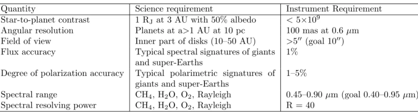
Table 1 summarizes the science requirements used to design the instrument concept described in the next section.
Table 1. Summary of the science requirements.
Quantity Science requirement Instrument Requirement
Star-to-planet contrast 1 RJat 3 AU with 50% albedo < 5×10⁹
Angular resolution Planets at a>1 AU at 10 pc 100 mas at 0.6 µm
Field of view Inner part of disks (10–50 AU) >500(goal 1000)
Flux accuracy Typical spectral signatures of giants
and super-Earths
1% Degree of polarization accuracy Typical polarimetric signatures of
giants and super-Earths
1–5%
Spectral range CH4, H2O, O2, Rayleigh 0.45–0.90 µm (goal 0.40–0.95 µm)
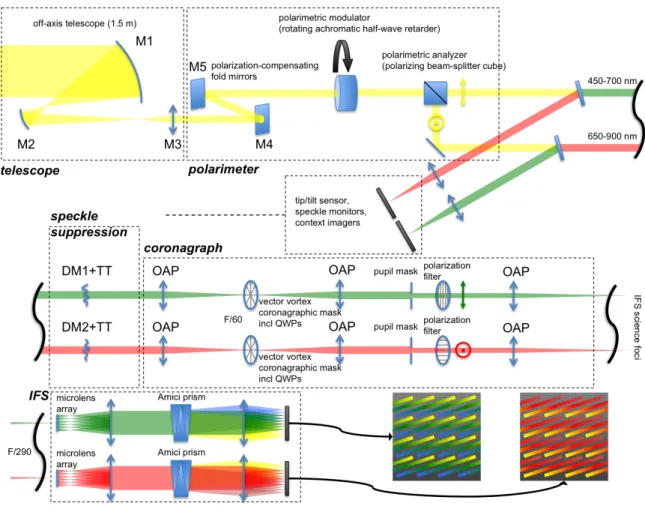
Figure 2. Conceptual design of the SPICES payload showing the main blocks: telescope, polarimeter, coronagraph and IFS. Only the main optics are shown here for sake of clarity (see text for details).
3. THE MISSION
3.1 Instrument concept
The general problem to image directly extrasolar planets near bright stars is well known and emblematic tech-niques like coronagraphy and wavefront control have been developed over the last 15 years to enable high-contrast imaging. The bottom line is to get rid of the diffraction pattern from the star to allow the detection of the faint planets. Nevertheless, SPICES has to tackle star/planet brightness ratio of typically 108–1010, which is 100 to
1000 times the contrast achieved with the next planet-finder instruments on the ground. Therefore, this chal-lenging mission requires a specific instrumentation, which is not available on any other facility present or future. Moreover, this very high contrast has to be achieved at angular separations of ∼0.200. Since SPICES has a small telescope (diameter 1.5 m), coronagraphs with small inner working angles (IWA) are required. Only phase-mask coronagraphs meet this constraint. We chose the vector vortex coronagraph [25, VVC], which offers a very high throughput (>90%). This has a strong impact on the instrument concept which is presented in Fig. 2. The instrument has an off-axis telescope with a good optical quality in order to limit the sensitivity of the VVC to mirror obscuration and wavefront aberrations. However, we need active wavefront correction with deformable mirrors (DM) to reach the contrast requirement (Sec. 4). Since SPICES will observe known planetary systems instead to search for new planets, the optical design is based on one DM only. A single DM will correct the wavefront aberrations in one half of the field of view, which will be adjusted to match the planet position. As VVC is a phase coronagraph, it is chromatic by definition, so we split the whole bandwith (0.45–0.9 µm) into
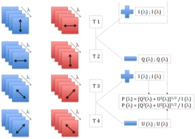
Figure 3. Illustration of the SPICES measurement concept. Data cubes (x, y, λ) are reconstructed for the blue and red IFS channels. Four sequences are obtained at different times T1, T2, T3, T4. At a given time the polarization directions are orthogonal between the channels. The direct sum of T1 and T2 data gives the intensity spectrum while two more sets of data (with 45◦and 135◦orientations) are needed to build Stokes vectors U and Q which define the polarized flux.
two spectral channels (0.45–0.70 µm / 0.65–0.90 µm) to reduce this issue. Each spectral channel includes a DM, a VVC and a micro-lenses based integral field spectro-polarimeter (IFS) with a 4k×4k detector. The IFS is similar to those developed now on the ground.26 The measurement of the aberrations is directly obtained at the
focal plane so that no differential aberrations occur and no supplementary channel for the wavefront sensing is needed. The IFS offers the capability to sense the wavefront in each spectral channel so that both phase and amplitude can be corrected accross half of the field of view. The wavefront control is achieved with the Electric Field Conjugation,27a specific algorithm to measure the aberrations, which provides a wavefront correction with
a quality/stability of the order of tens of picometers. As a goal, we propose a new concept, the Self Coherent Camera [28, SCC], for wavefront sensing that is being evaluated in the lab, but not yet at TRL 5 unlike our baseline algorithm. However, this device is very simple to implement and allows a better discrimination of plan-ets and speckles (see Refs. 29, 30, and the communication by Mazoyer et al. published in these proceedings).
Table 2. Overall requirements for the payload.
Parameters Values
Telescope Diameter (D) 1.5 m
Bandwidths specs (goal) 0.45–0.90 µm (0.40–0.95 µm)
Equivalent spatial resolution (goal) 62–120 mas (55–127 mas)
Blue channel / Red channel 0.45–0.70 µm / 0.65–0.90 µm
Observable Stokes parameters I, Q, U
Planet/Star contrast at 2 λ/D a few 10−9 Planet/Star contrast at 4 λ/D a few 10−10 Deformable mirror, nb. of elements 64×64 actuators Corrected field of view (blue/red channel) 600 / 800
Imaged field of view (blue/red channel) 900 / 1200
Static wavefront errors 20 nm rms
DM wavefront errors 10 pm rms
Final pointing accuracy 0.5 mas (goal 0.1 mas)
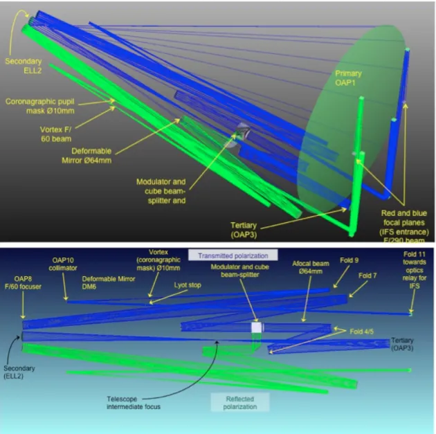
Figure 4. Top: General optical layout showing the implementation of the main components. Most of the optical elements are located below the M1-M2 segment while the IFS is deported at the back of the primary mirror. Bottom: detailed view of the instrument, as seen from above.
The integration times will be long, from some ten hours for a close Jupiter around a nearby bright star to one hundred of hours for a super-Earth.10 The frequency of wavefront sensing together with polarimetric modulation
will be faster to ensure a very high calibration and wavefront correction (from a few hours to 1 day).
Polarimetry is implemented in the design by inserting a rotating half-wave retarder as a modulator and a polarizing beam-splitter cube as an analyzer. They are placed after the primary mirror and some fold mirrors compensating the polarization of the former. Each channel has a polarimetric orientation assigned but the modulator allows to rotate a direction of polarization on the sky to the direction that the analyzer filters. The effect is that half of the light is sent to the detector at once, but the other half is used to sense the star position on the coronagraph with a precision of 0.1 mas. Therefore, the full coverage of the spectral band and polarimetric vectors requires four sets of observations with four positions of the modulator (Fig. 3). All SPICES sub-systems are close or above TRL 5. A full optical design is proposed in Fig. 4 but more work will be needed to provide a definitive concept. However, this is beyond the scope of this paper.
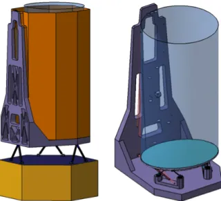
Figure 5. Opto-mechanical views of the telescope with the payload, showing in particular the L-shape base plate on which the optical elements are fixed. The dimension of the main telescope (without the platform) is 3350 × 1850 × 1540 mm. Design : Astrium-France.
3.2 Pointing strategy
The pointing requirement is an important aspect of the SPICES concept. At the instrument level, the alignment of the star onto the coronagraph must be very good to avoid stellar leakage and achieve the largest contrast. From simulations, we obtained a requirement of 0.1 mas at the level of the coronagraph over a timescale that is representative of the instrument stability. In addition, a telescope pointing of typically 2–10 mas is required to avoid beam walk on the primary and secondary, which would otherwise cause an unacceptable decorrelation of the wavefront over time. This value is similar to the JWST requirement.31 To meet these demanding accuracies, we propose a three-stage procedure. First, a coarse pointing is achieved by the spacecraft service module, within an accuracy of a few arcseconds (similar to Gaia and Herschel ). In the second stage, the spacecraft attitude control system (ACS) refines the pointing to a precision of 10 mas using the star position measurement provided by the payload itself (therefore limiting differential effects). Two solutions are considered: either the use of the light reflected by the filters as shown in Fig. 2 (saving thus all the light unused by the science channels), or the use of the starlight rejected by the coronagraph at the Lyot stop (achieving numerically a precision as good as 0.05 mas). Finally, the third stage of pointing corrects for the small tip tilt variations down to a precision of 0.1 mas using the error signal on the pointing detector. The usual way to do this is to make use of a fine steering mirror. A preferable solution for SPICES is to use a tip/tilt mount holding the DM, so that tip/tilt and higher order corrections are performed by the same optical element. The ACCESS proposal8 demonstrates the ability
of the telescope ACS to achieve the pointing specifications of stages 2 and 3.
3.3 Mission and spacecraft design
Section 2.2 describing the potential targets of SPICES indicates roughly that about 80–100 targets would consti-tute the core sample of SPICES for deep spectro-polarimetric characterization. A preliminary estimation gives a mission duration of three years.11 For thermal stability (high dimensional stability is required for the telescope
and instrument optics), target accessibility (avoidance of occultation of the sky by the Earth), and high data rate for the full mission, SPICES will be on an orbit around the Sun-Earth L2 Lagrangian point. A target will be accessible twice a year. The whole telescope is passively cooled at about 200 K, using special material like SiC to ensure a good stability and will point to the same target for a long duration (thermal variations are minimized), without any need to re-point the spacecraft for data transfer. But the current TRL5+ DMs operate at room temperature. This implies some thermal gradients, which require a special care for the thermal insulation.
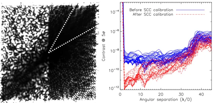
Figure 6. Left: Central part of a simulated no-noise image provided by the SPICES instrument (DM+VVC+SCC) at a wavelength of 0.675 µm (field of view 6×6 arcsec2, see Sec. 4 for the hypotheses). Due to amplitude aberrations, the DM correction occurs in one half of the field of view (here the right half). The calibration of the stellar residuals by the SCC is more efficient on a diagonal from the bottom left to the top right (see text). The white dotted line indicates the area used for the calculation of the radial profiles shown in the right panel. Right: 5-σ detection profiles of the instrument contrast achieved by SPICES for all spectral channels, before (blue solid lines) and after (red dashed lines) the SCC speckle calibration.
Figure 5 shows opto-mechanical views of the spacecraft with the payload designed by Astrium-France. The telescope core structure is constituted by a nearly SiC L-shape frame which provides easy fixation interfaces to the primary and secondary mirrors, the focal planes and optical items of the polarimeters and coronagraphs. In this way, the complete optical path is then fixed to this main structural frame while the whole telescope can tip up to 30◦ with respect to the plane normal to the Earth-Sun direction and rotate around the Sun direction.
4. NUMERICAL PERFORMANCE
We briefly discuss in this section the instrument performance that we obtained from numerical simulations. We refer the reader to the companion paper published in these proceedings and to Ref. 10. The main hypotheses are the following. We simulate an off-axis primary mirror of diameter 1.5 m, an achromatic VVC, a 64×64 DM and a SCC. The primary mirror is affected by phase aberrations corresponding to optical path differences of 20 nm rms and amplitude aberrations of 0.1%. The light is propagated with Fourier Transforms.32 We consider the whole bandwidth instead of the two spectral channels shown in Fig. 2. We split this bandwidth into 35 channels of the same width 0.013 µm. This provides a spectral resolution from 35 at the smallest wavelengths to 70 at the longest wavelengths, with a value of 50 at the central wavelength. We do not simulate the polarimeter. We assume that the wavefront aberrations are perfectly estimated by the SCC and projected onto the influence functions of the DM using the algorithm of Ref. 33. The wavefront aberrations will be corrected in one half of the field of view of size (N/2)(λ/D) × N (λ/D), where N is the number of DM actuators on one side so N = 64 (Fig. 6, left panel). We do not simulate the IFS and assume that the data cubes (x, y, λ) are reconstructed without numerical errors. However, we account for the flat field variations (0.5%) of the detector because the spectra provided by the IFS are dispersed on different pixels. We assume a host star similar to the Sun and a global throughput of 16% (instrument throughput × quantum efficiency of the CCD). We account for the photon and read-out noise. The CCD has a read-out noise of 0.2 e- rms per pixel and a full well capacity of 300 000 e-. The maximum single exposure is set to 1 000 s. As mentioned in Sec. 3.1, the SCC provides a means to calibrate further the stellar residuals after the DM correction. This device uses the coherence property of the
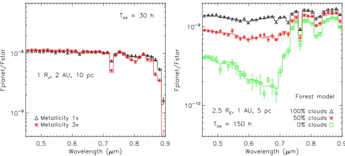
Figure 7. Left: Simulated (symbols) and theoretical (solid lines) spectra of Jupiters for metallicities of 1 and 3 (solar units). The median SNR measured on the spectrum is 30. Right: Same as the left figure but for forest super-Earths with different cloud coverages. The measured SNR is 25. All error bars are at 1σ.
Table 3. Signal-to-noise ratio (SNR) measured on the main features of the spectra of Fig. 7.
Jupiter Feature SNR CH4 band @ 0.62 µm >17 CH4 band @ 0.73 µm >15 CH4 band @ 0.79 µm >24 CH4 band @ 0.86 µm >9 Super-Terre Feature SNR O3band @ 0.54–0.64 µm ∼23 (100% clouds) H2O band @ 0.72 µm ∼28 (100% clouds) O2band @ 0.76 µm >5 H2O band @ 0.82 µm >23
stellar light to distinguish stellar residuals from planets.30 This calibration occurs in all the field of view but it
is more efficient on a diagonal as shown in the left panel of Fig. 6.
The right panel of Fig. 6 shows the radial profiles of the 5-σ instrument contrast against angular separation (λ = 0.675 µm) for all spectral channels, before and after the speckle calibration by the SCC. The radial profiles are calculated in the area delimited by the white dotted line in the left panel of the figure. We see that the detection limit after the DM is a few 10−9, which satisfies the contrast requirement at 2 λ/D (Table 2). However, the additional speckle subtraction achievable with the SCC is necessary to reach the requirement of ∼10−10 at a few λ/D (Table 2). The wavelength dispersion of the performance is due to the phase aberration dependence on wavelength (∝ λ−1) and the SCC calibration dependence on spectral resolution.29 The steep increase of the detection limit around 32 λ/D corresponds to the DM cut-off spatial frequency. This cut-off and the more efficient SCC calibration at small separations explain the contrast degradation with angular separation.
To illustrate the spectrometric performance of SPICES, we briefly discuss two typical cases of planet. The left panel of Fig. 7 compares measured (symbols) and theoretical (solid lines) spectra for Jupiters at 2 AU at 10 pc for two metallicity enhancements (models from Ref. 15). The error bars on the measurements are at 1 σ. The exposure time is determined so that the median SNR on the brightest spectrum (1 solar metallicity) is 30. The spectra mainly show methane features that are well recovered after an exposure time of 30 h (SNR > 9, left panel of Table 3). The metallicity effects are more important in the methane bands, in particular at 0.73 and 0.86 µm. SPICES is thus able to distinguish between gaseous giants with metallicity factors as small as 3 from their spectra. The right panel stands for super-Earths at 1 AU at 5 pc for different cloud coverage (models from Ref. 14). The median SNR on the brightest spectrum (100% clouds) is 25. The absorption lines are due to water, molecular oxygen and ozone. Here again the main features are recovered but for a longer exposure time
of 150 h (SNR > 5, right panel of Table 3). Our instrument can also constrain the cloud coverage of a telluric planet because the latter alters the spectra especially in the blue part of the bandwidth.
5. CONCLUSION
We presented a space coronagraphic mission named SPICES which was submitted to the ESA Cosmic Vision call for medium-class missions in 2010. SPICES aims to perform visible spectro-polarimetric analysis of known cold exoplanets, from gas giants to nearby super-Earths. It combines several techniques for high-contrast imaging in a single instrument designed to maximize the astrophysical return while reducing the risks. This mission is an improved proposal of the former SEE-COAST proposal submitted in 2007.34 The instrument was not selected
after the two calls because it was judged too expensive (cost/time of technological developments) with respect to the budget envelop allocated to a medium-class mission (∼450 Me). We will re-submit SPICES to the next Cosmic Vision call for proposals.
REFERENCES
[1] Howard, A. W., Marcy, G. W., Johnson, J. A., Fischer, D. A., Wright, J. T., Isaacson, H., Valenti, J. A., Anderson, J., Lin, D. N. C., and Ida, S., “The occurrence and mass distribution of close-in super-earths, neptunes, and jupiters,” Science 330, 653– (2010).
[2] Cassan, A., Kubas, D., Beaulieu, J.-P., Dominik, M., Horne, K., Greenhill, J., Wambsganss, J., Menzies, J., Williams, A., Jørgensen, U. G., Udalski, A., Bennett, D. P., Albrow, M. D., Batista, V., Brillant, S., Caldwell, J. A. R., Cole, A., Coutures, C., Cook, K. H., Dieters, S., Prester, D. D., Donatowicz, J., Fouqu´e, P., Hill, K., Kains, N., Kane, S., Marquette, J.-B., Martin, R., Pollard, K. R., Sahu, K. C., Vinter, C., Warren, D., Watson, B., Zub, M., Sumi, T., Szyma´nski, M. K., Kubiak, M., Poleski, R., Soszynski, I., Ulaczyk, K., Pietrzy´nski, G., and Wyrzykowski, L., “One or more bound planets per milky way star from microlensing observations,” Nature 481, 167–169 (2012).
[3] Seager, S. and Deming, D., “Exoplanet atmospheres,” ARA&A 48, 631–672 (2010).
[4] Barman, T. S., Macintosh, B., Konopacky, Q. M., and Marois, C., “Clouds and chemistry in the atmosphere of extrasolar planet hr8799b,” ApJ 733, 65 (2011).
[5] Kasper, M., Beuzit, J.-L., Verinaud, C., Gratton, R. G., Kerber, F., Yaitskova, N., Boccaletti, A., Thatte, N., Schmid, H. M., Keller, C., Baudoz, P., Abe, L., Aller-Carpentier, E., Antichi, J., Bonavita, M., Dohlen, K., Fedrigo, E., Hanenburg, H., Hubin, N., Jager, R., Korkiakoski, V., Martinez, P., Mesa, D., Preis, O., Rabou, P., Roelfsema, R., Salter, G., Tecza, M., and Venema, L., “Epics: direct imaging of exoplanets with the e-elt,” in [SPIE Conf. Series ], SPIE Conf. Series 7735, 77352E (2010).
[6] Boccaletti, A., Baudoz, P., Baudrand, J., Reess, J. M., and Rouan, D., “Imaging exoplanets with the coronagraph of jwst/miri,” AdSpR 36, 1099–1106 (2005).
[7] Enya, K., Kotani, T., Haze, K., Aono, K., Nakagawa, T., Matsuhara, H., Kataza, H., Wada, T., Kawada, M., Fujiwara, K., Mita, M., Takeuchi, S., Komatsu, K., Sakai, S., Uchida, H., Mitani, S., Yamawaki, T., Miyata, T., Sako, S., Nakamura, T., Asano, K., Yamashita, T., Narita, N., Matsuo, T., Tamura, M., Nishikawa, J., Kokubo, E., Hayano, Y., Oya, S., Fukagawa, M., Shibai, H., Baba, N., Murakami, N., Itoh, Y., Honda, M., Okamoto, B., Ida, S., Takami, M., Abe, L., Guyon, O., Bierden, P., and Yamamuro, T., “The spica coronagraphic instrument (sci) for the study of exoplanets,” AdSpR 48, 323–333 (2011).
[8] Trauger, J., Stapelfeldt, K., Traub, W., Krist, J., Moody, D., Mawet, D., Serabyn, E., Henry, C., Brugarolas, P., Alexander, J., Gappinger, R., Dawson, O., Mireles, V., Park, P., Pueyo, L., Shaklan, S., Guyon, O., Kasdin, J., Vanderbei, R., Spergel, D., Belikov, R., Marcy, G., Brown, R. A., Schneider, J., Woodgate, B., Egerman, R., Matthews, G., Elias, J., Conturie, Y., Vallone, P., Voyer, P., Polidan, R., Lillie, C., Spittler, C., Lee, D., Hejal, R., Bronowicki, A., Saldivar, N., Ealey, M., and Price, T., “Access: a concept study for the direct imaging and spectroscopy of exoplanetary systems,” in [SPIE Conf. Series ], SPIE Conf. Series 7731, 773128 (2010).
[9] Guyon, O., Shaklan, S., Levine, M., Cahoy, K., Tenerelli, D., Belikov, R., and Kern, B., “The pupil mapping exoplanet coronagraphic observer (peco),” in [SPIE Conf. Series ], SPIE Conf. Series 7731, 773129 (2010).
[10] Maire, A.-L., Galicher, R., Boccaletti, A., Baudoz, P., Schneider, J., Cahoy, K., Stam, D., and Traub, W., “Atmospheric characterization of cold exoplanets using a 1.5-m coronagraphic space telescope,” A&A 541, A83 (2012).
[11] Boccaletti, A., Schneider, J., Traub, W., Lagage, P.-O., Stam, D., Gratton, R., Trauger, J., Cahoy, K., Snik, F., Baudoz, P., Galicher, R., Reess, J.-M., Mawet, D., Augereau, J.-C., Patience, J., Kuchner, M., Wyatt, M., Pantin, E., Maire, A.-L., V´erinaud, C., Ronayette, S., Dubreuil, D., Min, M., Rodenhuis, M., Mesa, D., Belikov, R., Guyon, O., Tamura, M., Murakami, N., and Beerer, I. M., “Spices: Spectro-polarimetric imaging and characterization of exoplanetary systems,” Exp. Astron. (2012). [arXiv:1203.0507].
[12] Cockell, C. S., Herbst, T., L´eger, A., Absil, O., Beichman, C., Benz, W., Brack, A., Chazelas, B., Chelli, A., Cottin, H., Coud´e du Foresto, V., Danchi, W., Defr`ere, D., den Herder, J.-W., Eiroa, C., Fridlund, M., Henning, T., Johnston, K., Kaltenegger, L., Labadie, L., Lammer, H., Launhardt, R., Lawson, P., Lay, O. P., Liseau, R., Martin, S. R., Mawet, D., Mourard, D., Moutou, C., Mugnier, L., Paresce, F., Quirrenbach, A., Rabbia, Y., Rottgering, H. J. A., Rouan, D., Santos, N., Selsis, F., Serabyn, E., Westall, F., White, G., Ollivier, M., and Bord´e, P., “Darwin – an experimental astronomy mission to search for extrasolar planets,” Exp. Astron. 23, 435–461 (2009).
[13] Martin, S., Ksendzov, A., Lay, O., Peters, R. D., and Scharf, D. P., “Tpf-interferometer: a decade of development in exoplanet detection technology,” in [SPIE Conf. Series ], SPIE Conf. Series 8151, 81510D (2011).
[14] Stam, D., “Spectropolarimetric signatures of earth-like extrasolar planets,” A&A 482, 989–1007 (2008). [15] Cahoy, K. L., Marley, M. S., and Fortney, J. J., “Exoplanet albedo spectra and colors as a function of
planet phase, separation, and metallicity,” ApJ 724, 189–214 (2010).
[16] Fortney, J., Marley, M., Saumon, D., and Lodders, K., “Synthetic spectra and colors of young giant planet atmospheres: Effects of initial conditions and atmospheric metallicity,” ApJ 683, 1104–1116 (2008). [17] Tinetti, G., Cash, W., Glassman, T., Keller, C., Oakley, P., Snik, F., Stam, D., and Turnbull, M.,
“Char-acterization of extra-solar planets with direct-imaging techniques,” in [astro2010: The Astronomy and As-trophysics Decadal Survey ], ArXiv AsAs-trophysics e-prints 2010, 296 (2009).
[18] Schneider, J., Dedieu, C., Le Sidaner, P., Savalle, R., and Zolotukhin, I., “Defining and cataloging exoplan-ets: the exoplanet.eu database,” A&A 532, A79+ (2011).
[19] Pepe, F., Lovis, C., S´egransan, D., Benz, W., Bouchy, F., Dumusque, X., Mayor, M., Queloz, D., Santos, N. C., and Udry, S., “The harps search for earth-like planets in the habitable zone. i. very low-mass planets around hd 20794, hd 85512, and hd 192310,” A&A 534, A58 (2011).
[20] Mayor, M., Pepe, F., Queloz, D., Bouchy, F., Rupprecht, G., Lo Curto, G., Avila, G., Benz, W., Bertaux, J.-L., Bonfils, X., Dall, T., Dekker, H., Delabre, B., Eckert, W., Fleury, M., Gilliotte, A., Gojak, D., Guzman, J. C., Kohler, D., Lizon, J.-L., Longinotti, A., Lovis, C., Megevand, D., Pasquini, L., Reyes, J., Sivan, J.-P., Sosnowska, D., Soto, R., Udry, S., van Kesteren, A., Weber, L., and Weilenmann, U., “Setting new standards with harps,” Msngr 114, 20–24 (2003).
[21] Pepe, F. A., Cristiani, S., Rebolo Lopez, R., Santos, N. C., Amorim, A., Avila, G., Benz, W., Bonifacio, P., Cabral, A., Carvas, P., Cirami, R., Coelho, J., Comari, M., Coretti, I., de Caprio, V., Dekker, H., Delabre, B., di Marcantonio, P., D’Odorico, V., Fleury, M., Garc´ıa, R., Herreros Linares, J. M., Hughes, I., Iwert, O., Lima, J., Lizon, J.-L., Lo Curto, G., Lovis, C., Manescau, A., Martins, C., M´egevand, D., Moitinho, A., Molaro, P., Monteiro, M., Monteiro, M., Pasquini, L., Mordasini, C., Queloz, D., Rasilla, J. L., Rebord˜ao, J. M., Santana Tschudi, S., Santin, P., Sosnowska, D., Span`o, P., Tenegi, F., Udry, S., Vanzella, E., Viel, M., Zapatero Osorio, M. R., and Zerbi, F., “Espresso: the echelle spectrograph for rocky exoplanets and stable spectroscopic observations,” in [SPIE Conf. Series ], SPIE Conf. Series 7735, 77350F (2010). [22] Wittenmyer, R. A., O’Toole, S. J., Jones, H. R. A., Tinney, C. G., Butler, R. P., Carter, B. D., and Bailey,
J., “The frequency of low-mass exoplanets. ii. the ”period valley”,” ApJ 722, 1854–1863 (2010).
[23] Mayor, M., Udry, S., Lovis, C., Pepe, F., Queloz, D., Benz, W., Bertaux, J.-L., Bouchy, F., Mordasini, C., and Segransan, D., “The harps search for southern extra-solar planets. xiii. a planetary system with 3 super-earths (4.2, 6.9, and 9.2 mearths),” A&A 493, 639–644 (2009).
[24] Casertano, S., Lattanzi, M. G., Sozzetti, A., Spagna, A., Jancart, S., Morbidelli, R., Pannunzio, R., Pour-baix, D., and Queloz, D., “Double-blind test program for astrometric planet detection with gaia,” A&A 482, 699–729 (2008).
[25] Mawet, D., Serabyn, E., Liewer, K., Hanot, C., McEldowney, S., Shemo, D., and O’Brien, N., “Optical vectorial vortex coronagraphs using liquid crystal polymers: theory, manufacturing and laboratory demon-stration,” Opt. Express 17, 1902–1918 (2009).
[26] Antichi, J., Dohlen, K., Gratton, R. G., Mesa, D., Claudi, R. U., Giro, E., Boccaletti, A., Mouillet, D., Puget, P., and Beuzit, J.-L., “Bigre: A low cross-talk integral field unit tailored for extrasolar planets imaging spectroscopy,” ApJ 695, 1042–1057 (2009).
[27] Give’on, A., Kern, B., Shaklan, S., Moody, D. C., and Pueyo, L., “Broadband wavefront correction algorithm for high-contrast imaging systems,” in [SPIE Conf. Series ], SPIE Conf. Series 6691, 66910A (2007). [28] Galicher, R., Baudoz, P., and Rousset, G., “Wavefront error correction and earth-like planet detection by a
self-coherent camera in space,” A&A 488, L9–L12 (2008).
[29] Galicher, R., Baudoz, P., Rousset, G., Totems, J., and Mas, M., “Self-coherent camera as a focal plane wavefront sensor: simulations,” A&A 509, A31+ (2010).
[30] Baudoz, P., Boccaletti, A., Baudrand, J., and Rouan, D., “The self-coherent camera: a new tool for planet detection,” in [Direct Imaging of Exoplanets: Science & Techniques ], Aime, C. and Vakili, F., eds., IAU Colloq. 200, 553 (2006).
[31] Nelan, E., “Jwst science instrument target acquisition concepts,” Tech. Rep. JWST-STScI-000405 (2005). [32] Soummer, R., Pueyo, L., Sivaramakrishnan, A., and Vanderbei, R. J., “Fast computation of lyot-style
coronagraph propagation,” Optics Express 15, 15935 (2007).
[33] Bord´e, P. J. and Traub, W. A., “High-contrast imaging from space: Speckle nulling in a low-aberration regime,” ApJ 638, 488–498 (2006).
[34] Schneider, J., Boccaletti, A., Mawet, D., Baudoz, P., Beuzit, J.-L., Doyon, R., Marley, M., Stam, D., Tinetti, G., Traub, W., Trauger, J., Aylward, A., Cho, J. Y.-K., Keller, C.-U., Udry, S., and the See-coast Team, “Super earth explorer: a coronagraphic off-axis space telescope,” Exp. Astron. 23, 357–377 (2009).