HAL Id: hal-03197693
https://hal-imt-atlantique.archives-ouvertes.fr/hal-03197693
Submitted on 14 Apr 2021
HAL is a multi-disciplinary open access
archive for the deposit and dissemination of
sci-entific research documents, whether they are
pub-lished or not. The documents may come from
teaching and research institutions in France or
abroad, or from public or private research centers.
L’archive ouverte pluridisciplinaire HAL, est
destinée au dépôt et à la diffusion de documents
scientifiques de niveau recherche, publiés ou non,
émanant des établissements d’enseignement et de
recherche français ou étrangers, des laboratoires
publics ou privés.
Estimation of spectrum valuation for 5G dynamic
frequency allocation and auctions
Ayman Chouayakh, Aurélien Bechler, Isabel Amigo, Loutfi Nuaymi, Patrick
Maillé
To cite this version:
Ayman Chouayakh, Aurélien Bechler, Isabel Amigo, Loutfi Nuaymi, Patrick Maillé. Estimation of
spectrum valuation for 5G dynamic frequency allocation and auctions. VTC2021-Spring, Apr 2021,
Helsinki (Online), Finland. �hal-03197693�
Estimation of spectrum valuation for 5G dynamic
frequency allocation and auctions
Ayman Chouayakh
∗, Aur´elien Bechler
∗, Isabel Amigo
†, Loutfi Nuaymi
†, Patrick Maill´e
†∗Orange Labs, Chatillon, France
† IMT Atlantique, Brest, Nantes and Rennes, France
Email:{ayman.chouayakh, aurelien.bechler}@orange.com Email: {isabel.amigo, loutfi.nuaymi, patrick.maille}@imt-atlantique.fr
Abstract—The high data rates and diversity of services in 5G require a flexible and efficient use of all the available frequencies. In 5G networks, new approaches of dynamic spectrum sharing will be deployed, allowing Mobile Network Operators (MNOs) to access other incumbents’ spectrum, after obtaining a license from the regulator. The attribution of licenses will be made via auction mechanisms valid for given geographical areas and durations. To determine how to bid, each MNO has to estimate his valuation for spectrum i.e., how much he is willing to pay for spectrum. In this paper, we propose a model for estimating that valuation. The model is based on Markov chain modeling of user behavior, to compute the MNO satisfaction as a function of the obtained spectrum. We then illustrate our method by applying it to real operator data.
I. INTRODUCTION
Accommodating exploding data traffic is among the greatest challenges for fifth generation (5G) networks. According to some estimations, data rates will be multiplied by 10 compared to 4G [1], while latency must go down to one millisecond or less. 5G use cases can be mapped to three different classes: i) Machine-Type Communications (MTC) will create an environment of smart cities based on a new concept called internet of everything [2], ii) Ultra-Reliable Low-Latency Communications (URLLC) will enable connected autonomous vehicles and other latency-sensitive services, and iii) enhanced Mobile BroadBand (eMBB) will offer high transmission rates. According to [3], cellular network capacity may need to deliver as much as 1000 times the capacity of 4G. Accom-modating that traffic needs much larger bandwidths than the actual ones.
Currently some incumbent holders (through a licence) of some frequencies (e.g., military, satellites, some commercial users), do not always use all their spectrum: usage varies with time and geographical location [4]. Hence there is some room for improvement which has given rise to the idea of Licensed Shared Access (LSA). The concept involves three stakehold-ers: the owner of a bandwidth (the incumbent), the secondary user which is called the LSA licensee, and the regulator [5]. The first candidate bandwidth for the LSA concept is the 2.3 − 2.4 GHz bandwidth. This frequency band is used by different incumbents in Europe (e.g., in France it is used by the military). Under the LSA approach, the secondary user
needs to obtain a license from the regulator before accessing the spectrum of the incumbent. In general the attribution of licences is done via two approaches: administrative approaches (e.g., comparison of candidacies or beauty contests in which a committee sets a number of criteria and the license is attributed to the Mobile Network Operator (MNO) with the best mix of those criteria) and market-based approaches (e.g., auctions). Administrative approaches are used when demand is below supply or when the regulator and MNOs can find an agreement to split spectrum at some price [6]. However, when we cannot satisfy all MNOs or there is a lack of resources, auctions are the fairest means for spectrum assignment: since the regulator ignores the valuation that the bandwidth has for operators, a natural approach is to have them declare that valuation through an auction mechanism, so that the regulator allocates resources in the most efficient way, i.e., to maximize the resulting valuation to the market. The 2.3 − 2.4 GHz is considered as a very valuable (and therefore scarce) resource thanks to its ability to propagate far and offer high capacity. Thus, auctions [7] are more adequate to allocate spectrum to MNOs in this context.
In the LSA concept, the allocation will be made at the base station level [7]. Before participating in the auction, each base station has to compute its valuation [7], [8]. A specificity of LSA is that the allocation needs to work at a fast time scale, since the availability of LSA spectrum will be changed by the incumbent possibly several times per hour, and spectrum has to be allocated as soon as the incumbent releases his spectrum in order to improve its use. Therefore, a model which computes dynamically that valuation needs to be developed. However, computing that valuation is challenging because many factors can affect it [9]. Several approaches can be found in the literature to estimate spectrum valuation. One is the engineering value [10], which represents the savings in infrastructure from using additional spectrum instead of expanding the existing network to obtain the same capacity. Another approach is the strategic value, which represents the expected market position resulting from the additional spectrum [11]. Finally, the economic value [12] represents the profits earned by using the additional spectrum (revenue surplus from the market). In [9], [13] the authors identify
the key elements that impact the economic valuation. In [14] the authors propose a model based on user satisfaction in order to compute the economic valuation. In [15], based on the model proposed in [14] and using a Poisson process for modeling arrivals [16], the authors propose a more detailed model. In this paper we propose a new model, inspired by those previous works, by extending the model proposed in [15] to consider several types of users (typically, real-time users and file-downloading users, with different requirements) instead of one.
II. LSASPECTRUM VALUATION MODEL
We present in this section our economic model. In [15], the authors assume that all users have the same activity (each one consumes a quantity of data exponentially distributed with mean m). In order to get closer to real life, we add a new type of users, whose connection duration does not depend of the quality they experience (we will assume it is exponentially distributed with mean µ1). Our model takes into account the duration of the license and the quantity of the LSA spectrum (intuitively the valuation for spectrum must be a non-decreasing function with the duration of the license and with the quantity of LSA spectrum), also the model takes into account the average income from users in the geographical area of interest (the revenue from a user may vary from country to country).
We denote by Wnthe normal bandwidth of a base station h
and by Wtot, the total bandwidth i.e., the package composed of
the normal bandwidth and the LSA bandwidth. The valuation v of the base station for the additional bandwidth is given by v = V (Wtot) − V (Wn), (1)
where V (Wtot) is the valuation of the total bandwidth and
V (Wn) is the valuation of the normal bandwidth. Now the
question is: given a bandwidth W , how to compute V (W )? We suppose that the valuation of a bandwidth during a period t is just the average revenue from a user multiplied by the average number of users during that period.
V (W ) = Nprev,˜ (2)
where ˜rev is the average revenue from a user and Np is the
average number of users served during t.
A. Average revenue per user versus user satisfaction
The higher the satisfaction of users, the higher the operator revenue [15]. The authors in [17] note that spectrum has more valuation in high-income regions. Combining those assump-tions we suggest, as in [15], the following representation of the average revenue from a user:
˜
rev = czuS,˜ (3)
where ˜S is the average satisfaction and cz
u is a constant in
euros per unit of satisfaction in a given geographical zone which depends on the average income of users of that zone.
B. User satisfaction as a function of QoS
It is common in the literature [15], [18] to express user satisfaction as a function of data rate. Results given in [19] suggest that user satisfaction keeps increasing with the data rate but more and more slowly. In [18] authors have proposed the following formulation of user satisfaction:
S = 1 − e−(dcomd ), (4)
where d is the data rate and dcom is a comfort data rate
(can be interpreted as the mean data rate beyond which user satisfaction exceeds 63% of the maximum satisfaction [14]). Other parameters (such as the bit error rate) can have an impact on user perceived QoS, but we will focus here on the average data rate.
Among the factors that can affect the average data rate of a user served by a Base Station (BS) h, we suppose that the main ones are:
• the total throughput D of BS h, that D depends on the bandwidth W and other factors such as the digital modulation;
• the number of users connected to BS h;
• the maximum number Nmax of users that can be served
simultaneously by BS h;
• the scheduling i.e., how resources are divided when there are n users connected to BS h (we suppose that when there are n users, resources are allocated in such a way that all users perceive the same data rate).
In the following, we provide a model which computes the average user satisfaction from those parameters (the final formula is given in (7)). We assume a Poisson arrival process, an consider two types of users.
• Type 1: those users (with arrival rate λ1) stay connected
for a duration exponentially distributed with mean 1µ so the service rate (the connection duration) is independent of the BS throughput (e.g., video conference)
• Type 2: those users (with arrival rate λ2) stay connected
until they finish downloading a given quantity of data, that we assume exponentially distributed with mean m so the service rate depends on the available BS throughput (e.g., downloading an application, loading a web page). At each instant, when there are n users, we suppose that resources are allocated in such a way that all users, indepen-dently of their type, perceive the same data rate. Therefore if there are i users of Type 1 and j users of Type 2, we can establish the following results:
• The departure rate for Type-1 users is µ1i,j = i × µ (i
users of Type 1 with individual departure rate µ).
• The departure rate µ2i,j for users of Type 2 depends
on their data rate. That data rate depends on the total throughput D and the total number of connected user (we have i + j users). There are j users of Type 2, the service rate of each one is his throughput divided by m: µ2i,j=
D i+j
m × j.
With those assumptions, the pair (i, j) of numbers of connected users of each type is a Markov process [20]. The
transition diagram for the specific case Nmax= 3 is drawn in
Fig. 1 (µsat = Dm). Note that for any non-null values of the
(0,0) (0,1) (0,2) (0,3) (1,0) (1,1) (1,2) (2,0) (2,1) (3,0) λ1 λ2 λ1 λ2 λ1 λ2 λ1 λ2 λ1 λ2 λ1 λ2 1µ 1µ 1µ 2µ 2µ 3µ 1µsat 1 (1+1)µsat 1 (1+2)µsat 2 (2+0)µsat 2 (2+1)µsat 3 (3+0)µsat
Fig. 1: Markov chain describing the evolution of (n1, n2) for
Nm= 3, where nk is the number of Type-k users.
parameters, the chain is irreducible and has a finite number of states, hence it admits a unique stationary distribution.
If λ1, λ2, D, m and Nmaxare known to the MNO, then we
can compute the service rates. We denote by Πi,jthe stationary
probability of there being i users of Type 1 and j users of Type 2. The associated balance equations of the Markov chain can be established as follows:
• (λ1+ λ2)Π0,0 = µ11,0Π1,0+ µ20,1Π0,1
• (λ1 + λ2 + µ1i,0)Πi,0 = µ1i+1,0Πi+1,0 + µ2i,1Πi,1 +
λ1Πi−1,0; i < Nmax • (λ1 + λ2 + µ20,j)Π0,j = µ20,j+1Π0,j+1 + µ11,jΠ1,j + λ2Π0,j−1; j < Nmax • λ1ΠNmax−1,0= µ 1 Nmax,0ΠNmax,0 • λ2Π0,Nmax−1 = µ 2 0,NmaxΠ0,Nmax
• (µ1i,j + µ2i,j)Πi,j = λ1Πi−1,j + λ2Πi,j−1; i + j =
Nmax; i, j < Nmax
• (λ1+ λ2+ µ1i,j + µ2i,j)Πi,j = λ1Πi−1,j+ λ2Πi,j−1+
µ1
i+1,jΠi+1,j+ µ1i,j+1Πi,j+1; 0 < i, j < Nmax
From those equations, we build a matrix A such that ΠA = Π then we look for the eigenvector of constant sign associated with 1 and we normalize it to find Π. Once Π is computed the average satisfaction of a client at his arrival time can be written as: e S = Nm−1 X k=0 ( k X i=0 Πi,k−i)(1 − exp( dk+1 dcom )) (5) with dk+1 = k+1D the data rate of each user when there are
k + 1 users. We suppose that the average revenue is inde-pendent of the service time. More specifically, as in [15], we assume that the average revenue of an accepted user is equal to the average satisfaction during the service time multiplied
by a constant in euros per unit of satisfaction. In addition, we suppose that the the average satisfaction during the service time is approximately equal to the average satisfaction at the arrival time. Also, in order to consider the refused users, we propose to penalize BS, as in [15], by subtracting pefrom its
revenue each time a user is rejected. Therefore, the average revenue ˜rev from a user can be approximated as:
˜
rev = czuS − Π˜ Nmaxpe (6)
Where ΠNmaxis the blocking probability. Finally, the valuation
of W during t is:
V (W ) = Np(czuS − Π˜ Nmpe) (7)
Where Np is the average number of users presented during
the period of the licence t. Fig. 2 summarizes the steps that we have done in order to compute the valuation.
Capacity Nmax, Throughput D, Arrival rates (λ1, λ2) Steady state probability of the Markov Process Π Average satisfaction ˜S Average revenue ˜rev valuation of W V (W )
Fig. 2: Steps for computing the valuation for the bandwidth during a period t
C. Illustration
In the following, we illustrate our model by a simple exam-ple. We fix Nmax = 100, czu = 1 euro/unit of satisfaction,
dcom = 5 Mb/s, t = 300 s and pe = 0.2 euro. We suppose
that all users are of Type 2 with m = 50 Mb and arrival rate λ. We fix three possible valuations for λ. For each valuation, we compute the valuation as a function of the throughput as shown in Fig. 3. Fig. 4 shows how to compute the valuation, for
50 100 0 500 1,000 1,500 Throughput (Mb/s) v aluation λ = 1 s−1 λ = 3 s−1 λ = 5 s−1
Fig. 3: valuation as a function of the throughput for Nmax=
100
λ = 5 s−1, when the normal bandwidth generates a throughput 40 Mb/s and the total bandwidth generates a 70 Mb/s.
That valuation seems to be important compared to the one where λ = 1 s−1, This can be interpreted as follows: with the
normal bandwidth and for λ = 1 s−1 users are satisfied so there is no need to additional bandwidth.
Dn50 Dtot 100 0 500 1,000 1,500 vi Throughput (Mb/s) v aluation λ = 5 s−1
Fig. 4: valuation of the additional spectrum when Dn = 40
(Mb / s), Dtot= 70(M b/s) and λ = 5 s−1
III. DERIVING THE VALUATION OF ALSABANDWIDTH IN REAL WORLD
In the following we show how to apply our model when real data are available. We suppose that there is a LSA bandwidth which can be used for a duration t = 2h from 7 : 00 to 9 : 00 in a particular geographical area (Montparnasse). Mont-parnasse is a Parisian district, close to a train station, which can lead to congestion on certain time slots and therefore it is a district where the temporary allocation of spectrum seems relevant. Fig. 5 represents base stations which are concerned1.
Fig. 5: Some base stations in Montparnasse region From real data, each base station has to compute its valuation. A. Available real data
In the following we present our available data (initially used for designing and planning infrastructure network) which are summarized in Table I and are shown in Fig. 6 - Fig. 9 (valuations are hidden for confidentiality reasons and are shown each 15 min from 7 : 00 to 9 : 00 AM) for a particular base station h of Orange located in Montparnasse region. In
1(taken from (https://www.antennesmobiles.fr))
Np Average number of presented users.
Qm Average consumed quantity per user (Mb)
Tm Average time of a session (s)
davg Average throughput per user (Mb/s)
TABLE I: Available parameters from real data.
addition, we know the maximum throughout (Dn) of base
station h and the maximum number of users (Nmax) that can
be served simultaneously (those parameters are independent of time).
7 : 00 7 : 30 8 : 00 8 : 30 9 : 00
Throughput
(Mb/s)
Fig. 6: Average throughput (Mb/s)
7 : 00 7 : 30 8 : 00 8 : 30 9 : 00
Number
of
users
Fig. 7: Average number of users
7 : 00 7 : 30 8 : 00 8 : 30 9 : 00
A
v
erage
duration
Fig. 8: Average duration of a user session (s)
7 : 00 7 : 30 8 : 00 8 : 30 9 : 00
A
v
erage
duration
Now, from those data we have to compute the valuation of the additional bandwidth. Since we have the available data per 15 min, we propose to compute the valuation for each 15 min (A similar reasoning can be done for any other period of time). The final valuation is the sum of those valuations.
From available data, we have to compute: λ1, λ2, µ and
µsat. Once those parameters are computed we can therefore
compute the valuation. The difficulty with our available data is that we can not distinguish between types of users as an exam-ple the average consumed quantity is per user independently of his type. However, we can make some key assumptions and approximations that may help us to solve that problem. B. Estimating parameters
In this section, we show how to compute the parameters of our model. We denote by λ = λ1 + λ2. First, we have
the average number of presented users each 15 min (since the available data are per 15 min but the model can be applied for any period of time), we suppose that λ = Np
15×60
• The average consumed quantity qavgcan be expressed as: 1 2(q avg 1 + q avg 2 ) = 1 2(q avg 1 + m) = q avg,
where q1avgis the average consumed quantity of a user of Type 1 which can be approximated as: q1avg= 1
µ× d avg. So finally: 1 2( 1 µ× d avg+ m) = qavg (8)
• Similarly, the average connection time tavg can be ex-pressed as: 1 2(t avg 1 + t avg 2 ) = 1 2( 1 µ+ t avg 2 ) = t avg ,
where tavg2 is the average connection time of a user of
Type 2 which can be approximated as tavg2 = dmavg,
therefore: 1 2( 1 µ+ m davg) = t avg (9)
From Eq. (8) and Eq. (9), we can compute µ and m. Now we need to compute λ1 and λ2. The average data rate of a user
can be expressed as:
Nmax X k=1 Πk D k = d avg (10) Πk= k P i=1
Πi,k−i is computed from the matrix A (constructed
from the balance equations). The matrix A depends on λ1, λ2,
µ and m. For instance we know µ, m and λ1+ λ2. Therefore
in the matrix A we replace µ and m by its valuations and λ2
by λ − λ1. We compute Πk as a function of λ1. Then from
the average throughout Eq. (10) we compute λ1. Finally, we
compute λ2= λ − λ1. To summarize, steps are:
1) We set λ = Np
15×60
2) We compute µ and m from Eq. (8) and Eq. (9). 3) We set λ2= λ − λ1 and we compute λ1from Eq. (10).
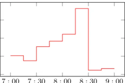
7 : 00 7 : 30 8 : 00 8 : 30 9 : 00
Fig. 7 valuation for spectrum each 15 min from 7 : 00 to 9 : 00 AM
4) We compute λ2 and finally we compute the stationary
distribution.
valuations of spectrum for each 15 min are shown in Fig. 7. The highest valuation is for the interval of time [8 : 15−8 : 30], this seems to be natural since there are many users who are served with low throughout. Finally, the valuation v for the LSA spectrum from 7 : 00 to 9 : 00 is the sum of valuations each 15 min .
IV. CONCLUSION
Valuing spectrum is a complex task because a lot of factors can be introduced. In our study, we have developed a new model based on the assumptions made in the literature and by adding a new type of users in order to get closer to real life. We have supposed that the valuation of a LSA bandwidth for a BS is its surplus i.e., the revenue with that bandwidth minus its revenue without that bandwidth. We have supposed that the revenue from a user depends on his satisfaction which depends on his data rate.
We have defined the number of connected users as a Markov process and show how to derive the steady state probability distribution so that from that probability distribution we can derive the average satisfaction and therefore the revenue from a user. In order to compute the steady state probability, we have supposed that there are two types of users and we have derived some theoretical results. Results suggest that the valuation of a LSA bandwidth varies and can be very high when users are not satisfied with the normal bandwidth. On the other hand, it can be very low when users are well satisfied with the normal bandwidth. we finally show how our model can be used to provide estimation of valuation when real data is available. As a next step, we enhance our model by considering the degree of rivalry between MNOs.
REFERENCES
[1] G. Ancans, V. Bobrovs, A. Ancans, and D. Kalibatiene, “Spectrum con-siderations for 5g mobile communication systems,” Procedia Computer Science, vol. 104, pp. 509–516, 2017.
[2] A. Ghanbari, O. Alvarez, and J. Markendahl, “Mtc value network for smart city ecosystems,” in 2016 IEEE Wireless Communications and Networking Conference Workshops (WCNCW), pp. 73–78, IEEE, 2016. [3] S. Talwar, D. Choudhury, K. Dimou, E. Aryafar, B. Bangerter, and K. Stewart, “Enabling technologies and architectures for 5g wireless,” in IEEE MTT-S International Microwave Symposium (IMS2014), pp. 1–4, 2014.
[4] V. Valenta, Z. Fedra, R. Marsalek, G. Baudoin, and M. Villegas, “Towards cognitive radio networks: Spectrum utilization measurements in suburb environment,” in Radio and Wireless Symposium, pp. 352–355, IEEE, 2009.
[5] M. Matinmikko, H. Okkonen, M. Malola, S. Yrjola, P. Ahokangas, and M. Mustonen, “Spectrum sharing using licensed shared access: the concept and its workflow for LTE-advanced networks,” IEEE Wireless Communications, vol. 21, pp. 72–79, May 2014.
[6] V. Valenta, R. Marˇs´alek, G. Baudoin, M. Villegas, M. Suarez, and F. Robert, “Survey on spectrum utilization in europe: Measurements, analyses and observations,” in 2010 Proceedings of the fifth international conference on cognitive radio oriented wireless networks and commu-nications, pp. 1–5.
[7] H. Wang, E. Dutkiewicz, G. Fang, and M. D. Mueck, “Spectrum Sharing Based on Truthful Auction in Licensed Shared Access Systems,” in Proc. of VTC Fall, (Boston, MA, USA), Jul 2015.
[8] A. Chouayakh, A. Bechler, I. Amigo, P. Maill´e, and L. Nuaymi, “Auction mechanisms for Licensed Shared Access: reserve prices and revenue-fairness tradeoffs,” in Proc. of IFIP WG PERFORMANCE, 2018. [9] J. Alden, “Exploring the value and economic valuation of spectrum,”
Rapport voor de ITU, 2012.
[10] A. A. W. Ahmed, Y. Yang, K. W. Sung, and J. Markendahl, “On the engineering value of spectrum in dense mobile network deployment sce-narios,” in 2015 IEEE International Symposium on Dynamic Spectrum Access Networks (DySPAN), pp. 293–296, IEEE, 2015.
[11] R. Sweet, I. Viehoff, D. Linardatos, and N. Kalouptsidis, “Marginal value-based pricing of additional spectrum assigned to cellular telephony operators,” Information Economics and Policy, vol. 14, no. 3, pp. 371 – 384, 2002.
[12] J. Markendahl, ¨O. M¨akitalo, B. G. M¨olleryd, and J. Werding, “Mobile broadband expansion calls for more spectrum or base stations-analysis of the value of spectrum and the role of spectrum aggregation,” 2010. [13] S. Malisuwan, N. Tiamnara, and N. Suriyakrai, “A study of spectrum
valuation methods in telecommunication services,” International Journal of Trade, Economics and Finance, vol. 6, no. 4, p. 241, 2015. [14] M. El Helou, S. Lahoud, M. Ibrahim, and K. Khawam,
“Satisfaction-based radio access technology selection in heterogeneous wireless networks,” in 2013 IFIP Wireless Days (WD), pp. 1–4, IEEE, 2013. [15] H. Kamal, M. Coupechoux, and P. Godlewski, “Inter-operator spectrum
sharing for cellular networks using game theory,” in 20th International Symposium on Personal, Indoor and Mobile Radio Communications, pp. 425–429, IEEE, 2009.
[16] O. J. Boxma and U. Yechiali, “Poisson processes,” Encyclopedia of statistics in quality and reliability, vol. 3, 2008.
[17] C. Bazelon and G. McHenry, “Spectrum value,” Telecommunications Policy, vol. 37, no. 9, pp. 737–747, 2013.
[18] N. Enderle and X. Lagrange, “User satisfaction models and scheduling algorithms for packet-switched services in umts,” in VTC 2003-Spring. The 57th IEEE Semiannual, vol. 3, pp. 1704–1709.
[19] Zhimei Jiang, H. Mason, Byoung Jo Kim, N. K. Shankaranarayanan, and P. Henry, “A subjective survey of user experience for data applications for future cellular wireless networks,” in Proceedings 2001 Symposium on Applications and the Internet, pp. 167–175, Jan 2001.
[20] R. A. Howard, Dynamic Programming and Markov Processes. Cam-bridge, MA: MIT Press, 1960.