Random thresholds for linear model selection

HAL Id: inria-00070434

https://hal.inria.fr/inria-00070434

Submitted on 19 May 2006

HAL is a multi-disciplinary open access

archive for the deposit and dissemination of

sci-entific research documents, whether they are

pub-lished or not. The documents may come from

L’archive ouverte pluridisciplinaire HAL, est

destinée au dépôt et à la diffusion de documents

scientifiques de niveau recherche, publiés ou non,

émanant des établissements d’enseignement et de

Marc Lavielle, Carenne Ludeña

To cite this version:

Marc Lavielle, Carenne Ludeña. Random thresholds for linear model selection. RR-5572, INRIA.

2005, pp.23. �inria-00070434�

ISRN INRIA/RR--5572--FR+ENG

a p p o r t

d e r e c h e r c h e

Thème COG

Random thresholds for linear model selection

Marc Lavielle — Carenne Ludeña

N° 5572

Marc Lavielle

_{, Carenne Ludeña}

Thème COG — Systèmes cognitifs Projet Select

Rapport de recherche n° 5572 — Mai 2005 — 23 pages

Abstract: A method is introduced to estimate the number of significant coefficients in non ordered model selection problems. The method is based on a convenient random centering of the partial sums of the ordered observations. Based on L_{−statistics methods we show consistency of the proposed estimator. An} extension to unknown parametric distributions is considered. The method is then applied to a regression model and interpreted as a random threshold procedure. Simulated examples are included to show the accuracy of the estimator.

Key-words: adaptive estimation, linear model selection, hard thresholding, random thresholding, L statistics.

This work was supported by ECOS Nord V00M03

∗_{Université René Descartes and Université Paris-Sud, France. e-mail: [email protected]} †_{IVIC, Venezuela E-mail: [email protected]}

Résumé : Une nouvelle méthode est proposée pour estimer le nombre de coefficients significatifs dans un problème de sélection de modèles. Cette méthode utilise un centrage aléatoire bien choisi des sommes cumulées partielles des observations ordonnées. En utilisant des propriétés des L-statistiques, nous montrons la consistance de l’estimateur proposé. Une extension à des distributions paramétriques inconnues est considérée. La procédure est ensuite appliquée à un modèle de régression et est interprétée comme une procédure de seuillage aléatoire. Des exemples numériques illustrent l’intérêt pratique de la méthode.

Mots-clés : estimation adaptative, sélection de modèle linéaire, seuillage dur, seuillage aléatoire, L-statistique.

1

Introduction

Consider the following model

yi= µi+ εi, i = 1, . . . , n

where (µi) is an unknown sequence of constants some of which are zero and (εi) are independent random

variables with common cumulative distribution Fε. The problem we study in this article is choosing the

significant, non zero, coefficients based on the observations (yi). Obviously, significant coefficients will be

those which are greater than a certain threshold, i.e. choose index i if

|yi| > τ. (1)

The choice of τ in (1) will depend on the distribution of the sequence (εi). So in practice τ must

be calibrated in terms of the data. A usual technique is to consider a sequence of thresholds (τj) for

values ranging from very small (many significant coefficients) to very big (few significant coefficients) and study the point where a substantial decrease in the number of significant coefficients occurs. Of course choosing the "right" τ is equivalent to choosing the "right" number k of significant coefficients, with the advantage that this can be done independently of the choice of (τj) by looking at the relative size of

the observations. Indeed, a jump in the relative size of the observations should indicate the existence of significant (not noise) coefficients.

This has been considered by a number of authors (see, for example, [6, 7, 10]) and many adaptive procedures aimed at studying the correct "jump point" have been developed.

A natural approach seems to consider the partial sums of the absolute (or squared) observations ordered decreasingly, and study the fluctuations of these partial sums around some kind of centering factor.

In this article we tackle this problem based on the use of order statistics by considering a convenient random centering: the conditional expectation, with respect to the total sum, of these partial sums. Even when this conditional expectation cannot be computed in a closed form, an exponential change of variable makes this centering possible. We then construct an L_{− statistic and study its weak convergence.} Empirical probability tables or simulated ones based on the limiting process can then be constructed to accept or reject the null hypothesis of all coefficients being equal to zero. If we reject the null hypothesis, further inspection of the test statistic yields the subset of significant coefficients. Indeed, we construct a test statistic based on the minimization of a certain functional of the conveniently centered partial sums and show consistency of the estimated number of significant coefficients under mild assumptions over the gap between significant and non significant coefficients.

The above method requires previous knowledge of Fε. In a parametric setting, Fε = Fε(· ; θ?), we

show that the proposed method can also address the case θ? _{unknown, assuming the existence of a}

consistent estimator of θ?_{. When θ}? _{is a scale parameter, an appropriate modification of the estimating}

procedure yields a scale free statistic, which is also shown to be consistent.

We then apply our method to the problem of estimating the number of significant coefficients for the regression problem

where f is an unknown function in some function space S and ηi are independent random variables

with variance σ2_{. A usual estimation procedure is to consider f ∈ L}2_{(µ) and a finite orthonormal}

system {φλ}Λ, with |Λ| = Mn. Denoting by hy, φji_n = 1/nPn_i=1yiφλ(xi) the empirical coefficients,

Donoho and Johnstone [5] in their seminal article proposed choosing only those coefficients whose absolute value exceeded a certain threshold u =

q

τ σ2_log(n)

n . This procedure has since been refereed to as hard

thresholding.

In a very interesting reinterpretation, Barron, Birge and Massart [2] study the problem of hard thresholding in the context of non ordered model selection based on the addition of a penalization term. Their arguments are combinatorial based on the complexity of the underlying linear spaces: the size of the set of all possible models of size k out of K is bounded by (eK/k)k_{and a logarithmic factor depending on}

K must be introduced in order to bound the probabilities. In terms of (1) our observations would now be the empirical coefficientshy, φji_n. Of course, except for the case ηi ∼ N(0, σ2), the empirical coefficients

will not be necessarily independent, although uncorrelated, so that the problem does not comply to our assumptions. However, in practice the method works well. As discussed in section 4.3, our method can be interpreted as a random threshold procedure .

The article is organized as follows: in section 2 we introduce the problem and basic notation as well as the proposed test procedure. In section 3 we state and prove theoretical results that justify our procedure, namely consistency of the selected subset of significant coefficients. In section 4.3 we consider certain extensions which include the parametric distribution case, an application to the problem of non ordered linear model selection for the regression setting and interpret out testing scheme in terms of a random penalization procedure. In section 5 we present simulated examples.

2

Describing the procedure

2.1

A first hypothesis testing procedure

Assume we observe yi= µi+ εi. Variables εiare assumed to be independent and identically distributed

with common cumulative distribution Fε. We begin by assuming that the cumulative distribution function

F_|ε|of the|εi|’s is known. In section 4 we will deal with the unknown F_|ε| case.

Given the collection (yi; 1≤ i ≤ n), we are interested in this section in testing if all the µi’s are null

or not. Thus, we introduce the following hypothesis: Null hypothesis:

H_{0 : µi ≡ 0 for i = 1, . . . , n.} Alternative hypothesis:

H_{1 : there exists a non empty subset I of{1, 2, . . . , n} such that µi6= 0 for i ∈ I.} Then, the test procedure is defined as follows:

ii) For i = 1, . . . , n, let X(i)=− log

¡

1_{− F|ε|}(_|y(i)|)

¢ , iii) Let Tj=Pji=1X(i)and Qj= EH0(Tj|Tn).

iv) Define the test statistic Dn = maxj|Tj− Qj|/√n. We will reject the null hypothesis if Dn > dα,

where dα is defined in Section 3.

Remark 1: Under the null hypothesis, the sequence (X(i)) is a decreasing sequence of exponential random

variables with parameter 1. Then, the conditional expectation EH0(Tj|Tn) can easily be computed using

the following proposition (the proof is given in the appendix):

Proposition 2.1 Assume X(1), X(2), . . . , X(n) is an ordered sequence of Exp(1) random variables,

with X(1)≥ X(2)≥ . . . X(n). For any 1≤ j ≤ n, let Tj=Pj_i=1X(i). Then, for any j≤ K ≤ n,

E¡X(i) ¢ = n X `=1 1 ` (2) E (Tj) = j + j n X i=j+1 1 i (3) E (Tj|TK) = E (Tj) E (TK) TK. (4)

Remark 2: The distribution of the test statistic Dn cannot be computed in a closed form. Nevertheless,

the following standard result will allow us to construct probability tables (the proof is given in the Appendix):

Theorem 2.1 Assume X(1), X(2), . . . , X(n) is an ordered sequence of Exp(1) random variables, with

X(1) ≥ X(2) ≥ . . . X(n). For any 1 ≤ j ≤ n, let Tj =Pji=1X(i). Introduce for t ∈ [0, 1] the random

process dn(t) = T[nt]−E

¡ T[nt]|Tn

¢

. Then, _√1

ndn(t), as a stochastic process indexed on t∈ [0, 1], converges

in distribution to a zero mean Gaussian process ∆ with covariance function defined by E (∆(t)∆(s)) =

Z 1 0

Z 1 0

[(1− u) ∧ (1 − v) − (1 − u)(1 − v)][1I[0,t](u)− t + t log(t)]

×[1I[0,s](v)− s + s log(s)]dG−1(u)dG−1(v),

where G(x) is the distribution function of an exponential r.v.

Using Theorem 2.1, we can conclude that statistic Dn defined in the test procedure converges weakly to

∆_∞= supt∆(t). Then, dα is defined as the α quantile of ∆∞.

Remark 3: Instead of assuming that the distribution of the _|εi| is known, we can assume that there

exists an increasing continuous function h : R+_{→ R}+ _{such that the cumulative distribution function F} h

of h(|ε|) is known. Then, X(i)is defined as − log

¡

1− Fh(h(|y(i)|))

¢

. Without any loss of generality, we will consider the case h = id in the following.

Remark 4: A uniform change of variable can also be used, by setting X(i) = F|ε|(|y(i)|). Indeed, the

conditional expectation of Tj can also be computed here:

E (Tj|TK) = j(K− j)

K + 1 +

j(j + 1) K(K + 1)TK

2.2

Choosing the right coefficients

If we reject the null hypothesis, the next step is to select the significant coefficients.

Let s be the one to one mapping from_{{1, 2, . . . , n} to {1, 2, . . . , n} defined by Y}s(i)= Y(i)(recall that

(Y(i)) is a decreasing sequence).

Then, define the set of alternative hypotheses: Alternative hypothesis:

H_{1(k) : there exists a subset Ik ⊂ {1, 2, . . . , n} such that,} - for any i_{∈ I}k, s(i)≤ k and EH1(k)(Yi)6= 0,

- for any i6∈ Ik, s(i)≥ k + 1 and EH1(k)(Yi) = 0,

Under H1(k), there are k significant coefficients and|y_(k+1)|, . . . , |y_(n)| have distribution F_|ε|. Then,

we define the following test procedure: i) For i = 1, . . . , n, let X(i)=− log

¡

1− F|ε|(|y(i)|)

¢ ,

ii) Let Kn be some positive integer. For 1≤ k ≤ n − Kn and 1≤ j ≤ Kn, compute

Tk,j = k+j X i=k+1 X(i), (5) Qk,j = EH1(k)(Tk,j|Tk,Kn) , (6) ηk = max 1≤j≤Kn |Tk,j− Qk,j| √ n . (7) iii) Let ˆ k = Arg min 1≤k≤n−Kn ηk

Remark 1: The `1 or the `2 norms can be used instead of the `∞ norm to define η by setting

ηk = n− 3 2 Kn X j=1 |Tk,j− Qk,j| or ηk= n−2 Kn X j=1 (Tk,j− Qk,j)2

Remark 2: Qk,j can easily be computed using the results of the previous section. Indeed, Let Bk,j,n= Ek (Tk,j) Ek(Tk,Kn) = j ³ 1 +Pn−k_i=j+11/i´ Kn ³ 1 +Pn−k_i=Kn+11/i´ (8)

Then, Proposition 2.1 yields Qk,j = Bk,j,nTk,Kn.

In order to state our main consistency result, we consider the following asymptotic framework:

AF1 There exists t?∈ (0, 1) and a subset Ik?

nof{1, 2, . . . , n} with k

?

n = [t?n], such that µi6= 0 if i ∈ Ik? n.

For all other index, µi = 0.

AF2 For any i _{∈ I}k?

n, |µi| ≥ αn, where αn → ∞ according to the distribution of the (εi). Let Φ(1)

be the distribution of max_1≤i≤n|εi| and (an, bn) such that Φ(1)(an+ bnx)→ W (x) for some fixed

distribution W . Then (αn) satisfies

αn− 2an

bn → ∞.

(9) AF3 Kn/n→ c such that 0 < c < 1 − t?.

We have the following result

Theorem 2.2 Let (un) be any positive and decreasing sequence such that √n un→ ∞. Then, under the

asymptotic framework defined by AF1, AF2,AF3, P ( ¯ ¯ ¯ ¯ ¯ ˆ k n− t ? ¯ ¯ ¯ ¯ ¯> un)→ 0. (10)

Moreover, for a > 0 there exist constants c1, c2 which depend on a such that if

un= c1αn √ log n 2√n + c2αnlog(n) 2n , then PH1(k?n) Ã |_nˆk− t?| > un ! ≤ 2e−a log(n)+ 2P µ max 1≤i≤n|εi| > αn ¶ . (11)

The proof of Theorem 2.2 is given in Section 3.

3

Proof of Theorem 2.2

Our procedure is based on two facts: a)under mild assumptions over the error distribution, if the null hypothesis is rejected, that is, if there is a group of significant coefficients and one of non significant coefficients, both groups of observations will be stochastically in order with high probability and b) for

two separate groups, separated at index k?

n = [t?n], Tkn,j− Qkn,j will only converge at rate

√_{n for index} kn such that|kn− kn?| = o(√n).

Set ui= yi for i∈ Ik?

n and vi = yi for i6∈ Ik?n. Thus (vi) is an i.i.d. sequence with distribution Fε.

We have the following lemma that assures that both collections are stochastically in order with high probability:

Lemma 3.1 Let (u(i)) and (v(i)) be the sequences (|ui|) and (|vi|) in a decreasing order. Then

P¡v(1)> u(k? n) ¢ → 0 and P ³ v(1)> αn 2 ´ → 0

Proof: By assumption (v(1)− an)/bn → W . On the other hand, let (˜vD i) be a sequence of i.i.d. r.v. with

distribution Fε. Then, P¡v(1)> u(k? n) ¢ ≤ P¡v(1)+ ˜v(1) > αn ¢ ≤ P¡v(1)> αn/2¢+ P¡v˜(1) > αn/2¢ ≤ 2P¡v(1)> αn/2 ¢ → 2W (αn/2_b− an n )_{→ 0. ¤}

Lemma 3.1 yields the (u(i)) and (v(i)) are stochastically in order with high probability . Let Ωn be

the subset of Ω where v(1)< αn/2 and u(k?

n)> αn/2. Clearly P (Ωn)→ 1. In what follows we will restrict

our proof to Ωn.

We will denote Ek() the expectation under H1(k) (instead of EH1(k)()). On the other hand, let

ai= E0

¡ X(i)

¢

=Pn<sub>`=1</sub>1/`.

1) Consider first the case k > k?

n. On Ωn, Tk,j− Qk,j = Tk,j− Bk,j,nTk,Kn = ¡Tk,j− Ek? n(Tk,j) ¢ − Bk,j,n ¡ T(k,Kn− Ek?n(Tk,Kn) ¢ + Ek? n(Tk,j)− Bk,jEk?n(Tk,Kn) = Rk,j+ Sk,j

We have decomposed the statistics Tk,j − Qk,j into a random part Rk,j and a deterministic part Sk,j.

First, let k = [tn] and j = [sn] for t ≤ s. As in Theorem 2.1, Rk,j1IΩn (normalized by

√_{n) as a} process indexed by (t, s) ∈ (0, 1)2 _{converges in distribution to a zero-mean Gaussian process Γ}

t,s =

On the other hand, Sk,j = Ek? n(Tk,j)− Ek(Tk,j) Ek(Tk,Kn) Ek? n(Tk,Kn) = Ek? n(Tk,j)− Ek(Tk,j)− Ek(Tk,j) Ek(Tk,Kn) ¡ Ek? n(Tk,Kn)− Ek(Tk,Kn) ¢ = j+k−k? n X i=j+1 ai− k−k? n X i=1 ai+ Bk,j,n   Kn+k−k_X ?n i=Kn+1 ai− k−k? n X i=1 ai   = k−k? n X i=1 ¡ ai+j− ai+ Bk,j,n(ai+Kn− ai) ¢

Thus, there exists a constant, γ > 0, which depends on c in [AF3], such that supj|Sk,j| ≥ γ(k − kn?) and

Pk? n ³ k? n− bk > n un ´ ≤ P¡ηk? n> sup ηk , (k− k ? n) > n un ¢ (12) ≤ P µ 2 sup k sup j Rk,j> infk supj |Sk,j| , (k − k ? n) > n un ¶ + P(Ωcn) ≤ P µ 2 sup k sup j Rk,j> γ n un ¶ + P(Ωcn) .

Because of the weak convergence of Rk,j1IΩn the above probability tends to zero when n goes to infinity.

2) Consider now the case k < k?

n. On Ωn, Tk,j− Qk,j = Tk,j− Bk,j,nTk,Kn = (1_{− B}k,j,n)Tk,k? n−k+ ¡ Tk? n,j− E ¡ Tk? n,j ¢¢ − Bk,j,n ¡ Tk? n,Kn− E ¡ Tk? n,Kn ¢¢ +E¡Tk? n,j ¢ − Bk,j,nE ¡ Tk? n,Kn ¢ = Ak,j+ Rk? n,j + Uk,j where Ak,j = (1− Bk,j,n)Tk,k?

n−k. Remark that over Ωn, |y(i)| > αn/2. Then, there exists c(αn) > 0

such that Tk,k?

n−k > c(αn)(k

?

n− k), thus Ak,j =O(kn?− k). On the other hand, Rk?

n,j1IΩn converges in

distribution to a zero-mean Gaussian process Γt?_,s. Consider now the bias term U_k,j:

Uk,j = Ek? n ¡ Tk? n,j ¢ −_EEk(Tk,j) k(Tk,Kn) Ek? n ¡ Tk? n,Kn ¢ = Ek? n ¡ Tk? n,j ¢ − Ek ¡ Tk? n,j ¢ − Ek ¡ Tk? n,j ¢ Ek(Tk,Kn) ¡ Ek? n ¡ Tk? n,Kn ¢ − Ek(Tk,Kn) ¢ +Ek?n ¡ Tk? n,Kn ¢ Ek(Tk,Kn) Ek¡Tk,k? n ¢ = j−k X i=j+k−k? n+1 ai− k? n−k X i=1 ai+ Ek¡Tk? n,j ¢ Ek(Tk,Kn) Kn X i=Kn+k−k?n+1 ai − Ek? n ¡ Tk? n,Kn ¢ Ek(Tk,Kn) k? n−k X i=1 ai.

Thus, there exists a constant δ > 0, which depends on c in [AF3], such that supj|Uk,j| ≥ δ(k − kn?) and

Pk? n ³ bk − k? n> n un ´

In order to show (11), sharper bounds on Pk? n

¡

supksupjRk,j > C n un

¢

are required for any given constant C. As above, we will restrict our attention to the set Ωn and drop this fact from the notation.

Consider first as above the case k > k?

n. Write, over Ωn, Rk,j = ¡Tk,j− Ek? n(Tk,j) ¢ − Bk,j,n¡Tk,Kn− Ek?n(Tk,Kn) ¢ = R(1)k,j+ R (2) k,j.

Remark supjBk,j,n= 1. So that supj|R (2)

k,j| = |Tk,Kn− Ekn?(Tk,Kn)|.

Let G denote the common distribution function of the collection (Xi). We can rewrite

Tk,Kn− Ek?n(Tk,Kn) = X i [Xi− Ek? n(Xi)]1I{G−1(1−K_n/n)<X_i}. Thus, Tk,Kn− Ekn?(Tk,Kn) αn/2

is the sum of independent bounded r.v. with variance bounded by 1, so that by Bennet’s inequality

P Ã supj|R (2) k,j| αn/2 > γ/2nun αn/2 ! ≤ P µ |Tk,Kn− Ek?n(Tk,Kn)| αn/2 > c1γ 2√2 p 2n log n +3c2γ 2 log n 3 ¶ ≤ e−(a+1) log(n)_,

choosing c2≥ 2(a+1)_3γ and c1≥ 2 √ 2√a+1 γ . Hence, summing in k P Ã sup k sup j<k+Kn R(2)_k,j> γ 2nun ! ≤ e−a log n_. For R(1)_k,j we have Tk,j− Ek? n(Tk,j) αn/2 =X i [Xi− Ek? n(Xi)]1I{G−1(1−j/n)<X_i}.

Hence in this case we must use a functional version of Bennet’s inequality (Theorem 7.3 in [4]) which yields P Ã supj|R (2) k,j| αn/2 > E Ã supj|R (2) k,j| αn/2 ! +√2xv +x 3 ! ≤ e−x_, for v ≥ n + 2E µ sup_j|R(2)k,j| αn/2 ¶

. Thus it remains to bound A = E µ

sup_j|R(2)k,j|

αn/2

¶

. This can be done using standard symmetrization and entropy techniques to obtain, A≤ 4√n log n, as the random entropy of the classA = {1IG−1(1−t),t∈[0,1]} (as it is a collection of increasing functions) is bounded by 2 log n.

As above, P Ã supj|R (1) k,j| αn/2 > γ/2nun αn/2 ! ≤ P µ₂ |Tk,j− Ek? n(Tk,j)| αn > 4 p n log n + q

2(a + 1) log n(n + 4pn log n) + (a + 1)log n 3 ¶ ≤ e−(a+1) log(n), choosing ci, i = 1, 2 appropriately. The case k < k? n follows analogously.

4

Some extensions

4.1

Unknown distribution

Assume now that the distribution Fε of the εi’s is a parametric distribution Fε(· ; θ?), but where the

parameter θ? _{is unknown. For any 0≤ k ≤ n − 1, let bθ}

k = bθ(y(k+1), y(k+2), . . . , y(n)) be an estimator of

θ. Let F_|ε|(· ; θ?_{) be the distribution of the|ε}

i|’s. We will consider the following assumptions:

F1 The cumulative distribution function F_|ε| is two times differentiable as a function of θ with a.e. strictly positive derivative at θ = θ?_.

F2 θ? belongs to some compact set Θ and there exists, under Hk?

n, a consistent estimator bθk?n =

b θ(y(k?

n+1), y(k?n+2), . . . , y(n)) of θ

?_.

F3 There exists (a, b) such that 0 < a < t? _{< b < 1 and a Lipschitz continuous function ˜θ defined on}

[a, b] such that, under Hk?

n, (bθ[tn]) converges uniformly on [a, b] in probability to ( ˜θ(t)).

Remark 1: under hypothesis F2 and F3, bθk?

n is a consistent estimator of ˜θ(t

?_{) = θ}?_.

Remark 2: When t < t?_{, convergence of bθ}

[tn] can be difficult to check with any estimator, since bθ[tn]

depends on some yi’s that are not distributed under distribution Fε. Nevertheless, it is possible to use

an estimator based on some empirical quantiles and that only depends on the smallest observations, that is, that depends only on the observations distributed under Fε.

For any θ_{∈ Θ, let X}i(θ) =− log¡1− F_|ε|(|yi|, θ)¢, and Tk,j(θ) =Pk+j_i=k+1X(i)(θ).

Then, we define the following procedure:

i) Let Kn≤ [(1 − b) n] be some positive integer. For [a n] ≤ k ≤ n − Kn,

2. for i = 1, . . . , n, let X(i)(bθk) =− log ³ 1_{− F|ε|}(_|y(i)|; bθk) ´ , 3. for 1_{≤ j ≤ K}n, compute Tk,j(bθk) = k+j X i=k+1 X(i)(bθk), Qk,j(bθk) = Bk,j,nTk,Kn(bθk), ηk(bθk) = max k+1≤j≤n |Tk,j(bθk)− Qk,j(bθk)| √_n . iii) Let ˆ k = Arg min an≤k≤bnηk(bθk)

Remark: Here, Qk,j(bθk) = Bk,j,nTk,Kn(bθk) is the conditional expectation of Tk,j, conditionally to Tk,Kn,

assuming that k?

n= k and that θ?= bθk.

Then, we have the following result, Theorem 4.1 Assume F1, F2, F3.

i) Introduce for t_{∈ [0, 1] and s ∈ [a, b] the random process} ˆ dn(t, s) = Tk? n,[Knt](bθ[ns])− EHk?_n ³ Tk? n,[Knt](bθ[ns])|Tk?n,Kn(bθ[ns]) ´ .

Then, ˆdn(t, s)/√n, as a stochastic process indexed on [0, 1]× [a, b], converges in distribution, under Hk? n,

to a zero mean Gaussian process (Λ(t, s)).

ii) Let (un) be any positive and decreasing sequence such that√n un→ ∞. Then, under the asymptotic

framework defined by AF1, AF2, AF3, PH1(k?n) ï¯_¯ ¯ ¯ ˆ k n− t ? ¯ ¯ ¯ ¯ ¯> un ! → 0. (13)

Proof: We first show i).

With the above notation, for any θ_{∈ Θ, let} Ψj(θ) = Tk?

n,j(θ)− Qk?n,j(θ)

Ψ0j(θ) =

∂Ψj

∂θ (θ) For any t∈ [0, 1] and s ∈ [a, b], let

ˆ

dn(t, s) = Ψ[nt](bθ[ns])

Using the same proof used for the convergence of (Ψ[nt](θ?))/√n (see the Appendix), we show that, for

any s∈ [a, b], (Ψ[nt](˜θ(s)))/√n and (Ψ0[nt](˜θ(s)))/

√_{n also converge to two zero-mean Gaussian processes.} Then, using hypothesis F3, bθ[ns] → ˜θ(s) uniformly over [a, b], and then, ( ˆdn(t, s)) converges to a zero

mean Gaussian process (Λ(t, s)).

We show now ii). For any θ _{∈ Θ, let a}i(θ) = EH0

¡ X(i)(θ)

¢

. Following the proof of Theorem 2.2, consider first the case k > k?

n. On Ωn, for any θ∈ Θ, Tk,j(θ)− Qk,j(θ) = ¡ Tk,j(θ)− Ek? n(Tk,j(θ)) ¢ − Bk,j,n ¡ Tk,Kn(θ)− Ek?n(Tk,Kn(θ)) ¢ + Ek? n(Tk,j(θ))− Bk,jEk?n(Tk,Kn(θ)) = Rk,j(θ) + Sk,j(θ)

As in Theorem 2.2, Rk,j (normalized by √n) as a process indexed by (t, s)∈ (0, 1)2 converges in

distri-bution on Ωn to a zero-mean Gaussian process Γt,s(θ).

On the other hand,

Sk,j(θ) = k−k? n X i=1 ¡ ai+j(θ)− ai(θ) + Bk,j,n(ai+Kn(θ)− ai(θ)) ¢

Thus, there exists a constant, γ > 0, which depends on a, b in [F3], such that supj|Sk,j(bθk)| ≥ (k − k?n)γ.

We conclude that Pk? n ³ k? n− bk > n un ´

→ 0 using the arguments used for Theorem 2.2. The case k < k? n

is identical. ¤.

4.2

The unknown variance case

When θ?_{is a scale parameter, i.e. F}

ε(y; θ?) = Fε(y/θ?; 1), we introduce the following procedure which is

scale invariant:

i) For i = 1, . . . , n, let X(i)=|y(i)|,

ii) Let Kn be some positive integer. For 1≤ k ≤ n − Kn and 1≤ j ≤ Kn, compute

Tk,j = k+j X i=1 X(i), (14) Qk,j = EH1(k) ³Pk+j i=kX(i) ´ EH1(k) ³Pk+Kn i=k X(i) ´ Tk,Kn, (15) ηk = max 1≤j≤Kn |Tk,j− Qk,j| √_n . (16) iii) Let ˆ ku= Arg min 1≤k≤n−Kn ηk

Remark: Notice, the minimization problem at hand is not changed if we consider |Tk,j−Qk,j|

σ√n , so the

procedure is indeed scale invariant. We have the following result, whose proof is omitted as it resembles quite closely that of Theorem 2.2.

Theorem 4.2 Let (un) be any positive and decreasing sequence such that √n un→ ∞. Then, under the

asymptotic framework defined by AF1, AF2,AF3, P (_|kˆu

n − t

?

| > un)→ 0.

Moreover, for a > 0 there exist constants c1, c2which depend on a such that if un= c1αn √ log n 2√n + c2αnlog(n) 2n then P (_|ˆku n − t ?

| > un)≤ 2e−a log n+ 2P ( max 1≤i≤n

|εi|

σ > αn).

4.3

Application to a regression problem

Consider as discussed in section 1 the following setting.

1. Assume we observe yi = f (xi) + εi for a fixed collection xi. Variables (εi) are assumed to be

independent and identically distributed with variance V ar(ε) = σ2_.

2. Associated to the collection (xi), we introduce the empirical inner productht, sin= 1n

P

it(xi)s(xi)

and its associated empirical norm_{k · k}n.

3. We are interested in approximating f in terms of a certain orthormal basis_{φλ}λ. We assume that

the basis is such that it is also orthonormal in the empirical norm_{h, in}. 4. Given the basis define the absolute empirical coefficients bβj =

¯ ¯hy, φji_n

¯

¯ √n. More generally, we could consider the collection of the transformed coefficients γj(h) = h( bβj/σ) for any given strictly

increasing function h such that there exists β satisfying h(ax) = aβ_{h(x) for any positive constant}

a.

In this section we are interested in the partial sums of the ordered variables bβ. If εi follows a

Gaus-sian distribution then yj =hy, φji_n√n/σ are independent normal variables and it is straightforward to

show that the procedure considered in section 4.2 can be applied. More precisely assume the following assumptions are satisfied

R1 εi are an i.i.d. collection of centered normal r.v. with variance σ2.

R2 _{φ1, . . . , φn} is orthonormal w.r.t. the empirical norm h, in.

R3 For any i∈ Ik?

n, | hf, φjin| > aσ

√

log 2n/√n, with a≥ 2√2. We have the following result,

Lemma 4.1 Assume AF1, AF3, R1, R2 and R3 hold true. Let ˆku, be the estimator defined in

section 4.2. Then, for b > 0 there exist constants c1, c2 which depend on a and b such that if un =

c1log(n) 2√n + c2log2(n) 2n then P (|kˆ_nu − t? | > un)≤ 2e−b log n+ 2e−(a/2− √ 2) log(n)_.

Proof: It follows directly from Theorem 4.2 by checking that if ²i, i = 1, . . . , n are independent standard

normal random variables, then

P ( max

1≤i≤n|²i| > a

√

2n)_{≤ e}−(a/2−√2) log(n).

4.4

Random thresholding

It is interesting we can link this procedure to a random thresholding one, or as in [2, 3] in terms of penalized estimation. This link clearly appears when we use the `2-norm to define ηk:

ηk = n−2

k+KXn

j=k+1

(Tk,j− Qk,j)2

Lemma 2.2 ensures that good choice for the cutpoint between significant and non significant coefficients is bk = arg min ηk. Thus, it is reasonable to assume we are looking from left to right to the first k such

that ηk > ηk−1. We will assume coefficients are significant while ηk < ηk−1. In order to develop this idea

we must understand how ηk− ηk−1looks like. We have

n2(ηk− ηk−1) = Kn X j=1 (Tk,j− Bk,jTk,Kn) 2 − K_Xn−1 j=1 Tk−1,j− Bk−1,jTk−1,n)2 = (Xk− Bk−1,kTk−1,k−1+Kn) 2₊ KXn−1 j=1 (Tk,j− Bk,jTk,Kn)) 2 − KXn−1 j=1 ³ Xk+ Tk,j− Bk,j(Xk+ Tk,Kn)(1 + o(1) ´2 ≈ (Xk− Bk−1,kTk−1,k−1+Kn) 2 + K_Xn−1 j=1 Xk2(1− Bk,j,n)2+ 2Xk(1− Bk,j,n)(Tk,j− Bk,j,nTk,k+Kn)

Hence coefficients will be significant approximatively until the first k such that Xk ≤ τk,n:= PKn−1 j=1 (Tk,j− Bk,jTk,Kn)(1− Bk,j,n) PKn−1 j=1 (1− Bk,j,n)2 .

Remark: If using the estimator bku, this would yield a scale free random estimator τk,nof the threshold

τ . In the regression case, we obtain the traditional hard threshold scheme ¯ ¯hy, φji_n ¯ ¯ >τk,n √_n

5

Numerical experiments

We consider here the model

yi= µi+ εi (17)

where (εi) is a collection of i.i.d. r.v.

5.1

_{Testing the null hypothesis H}

The distribution of Dn = maxj|Tj− bTj|/√n under H0is estimated by Monte-Carlo (using 5000 simulated

samples). Here, the (yi; 1≤ i ≤ n) are i.i.d. N (0, 1) r.v. We set X(i)=− log(1 − F (y2(i))) where F is the

cumulative distribution of a χ2(1) distribution. Then, (Tj), ( bTj) and Dn are computed as described in

Section 2.1.

Table 5.1 displays the estimated percentiles of order 0.50, 0.90, 0.95 and 0.99 obtained with different values of n. We see in this table that the distribution of Dn (except the tail) does not depend on n for

n_{≥ 20. In particular, P}H0(Dn> 0.65)≈ 0.05 for any n ≥ 20.

n\ α 0.50 0.90 0.95 0.99 20 0.27 0.55 0.67 0.93 50 0.29 0.55 0.65 0.82 500 0.29 0.56 0.65 0.83 5000 0.30 0.55 0.64 0.79

Table 1: Estimated percentiles of Dn under H0 obtained with different values of n

Using a level α = 5%, the test consist in rejecting the null hypothesis H0 if Dn > 0.65. We estimated

the power of this test, by simulating data under H1. Here, the (yi; 1 ≤ i ≤ n/5) are i.i.d. N (µ, 1) r.v.

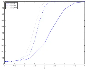
Figure 5.1 displays the estimated probability to reject the null hypothesis H0for different values of µ and

n.

5.2

Estimating the number of significant coefficients

5.2.1 A Gaussian example

In the following experiment, we have simulated 500 Gaussian random variables, with µi= 4 for 1≤ i ≤

0 0.5 1 1.5 2 2.5 3 3.5 4 0 0.1 0.2 0.3 0.4 0.5 0.6 0.7 0.8 0.9 1 µ n=50 n=500 n=1000

Figure 1: The estimated power of the 5% level test, for different values of µ and n. Assuming that the variance of the εi’s is known, we set

Xi=− log(1 − F (yi2))

where F is the cumulative distribution function of a χ2 _r.v.

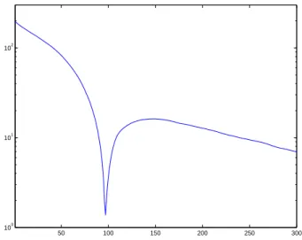
Then, we used the procedure described in Section 2.1. Figure 5.2.1 displays the two sequences (Tk)

and (Qk). We find Dn= 14.95 and reject the null hypothesis.

0 50 100 150 200 250 300 350 400 450 500 0

500 1000 1500

Figure 2: Example 1. The two sequences (Tk) and (Qk)

After rejecting the null hypothesis, we will estimate the number of significant coefficients, following the procedure described in Section 2.2. We use here K = 200. Then, for k = 1, 2, . . . , 300, we computed the sequences (Tk,j, 1≤ j ≤ 200) and (Qk,j, 1≤ j ≤ 200). Figure 5.2.1 displays these two sequences for

k = 70, k = 100 and k = 130. We see that (Tk,j) concentrates around its conditional expected value

(EH1(k)(Tk,j|Tk,200)) only for k = 100. A bias is clearly present for k = 70 and k = 130. The sequence

(ηk) defined by ηk = P200j=1(Tk,j− Qk,j)2/

√

n_{− k is displayed Figure 5.2.1. A minimum at ˆk = 97 is} obvious. 80 100 120 140 160 180 200 220 240 260 0 200 400 600 (a) 100 120 140 160 180 200 220 240 260 280 300 0 100 200 300 400 (b) 140 160 180 200 220 240 260 280 300 320 0 100 200 300 (c)

Figure 3: Example 1. The two sequences (Tk,j, 1≤ j ≤ 200) and (Qk,j, 1≤ j ≤ 200)

with (a) k = 70, (b) k = 100, (c) k = 130.

50 100 150 200 250 300 100

101 102

Figure 4: Example 1. The sequence (ηk) (in a semilog scale)

Repeating the same procedure with 100 simulated sequences, we obtained 100 values of ˆk. The mean value of ˆk is 97.6 and the standard deviation is 4.8.

If we consider now that the variance is unknown, we use the procedure described Section 4.1, estimating the variance under H1(k) by

b θk = 1 n_{− k} n X i=k+1 y2(i)

The results obtained when the variance is unknown are very similar than those obtained when the variance is known. The mean value of ˆk is 97.3 and the standard deviation is 5.1.

5.2.2 A Exponential example

In this second example, n = 500 again, but (εi) is a collection of Expo(1) i.i.d. r.v. Here, µiis uniformly

distributed in [3, 6] for 1_{≤ i ≤ 100, and µ}i= 0 for 101≤ i ≤ 500.

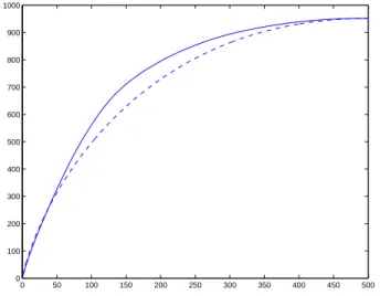
When the parameter of the exponential distribution is known, we use the procedure described Sec-tion 2.1, setting Xi= yi. Figure 5.2.2 displays the two sequences (Tk) and (Qk). We find Dn= 3.72 and

reject the null hypothesis.

0 50 100 150 200 250 300 350 400 450 500 0 100 200 300 400 500 600 700 800 900 1000

Figure 5: Example 2. The two sequences (Tk) and (Qk)

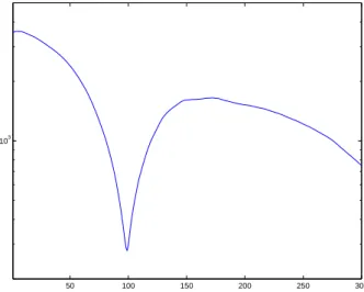
The number of significant coefficients is estimated as before. Figure 5.2.2 displays these two sequences (Tk,j, 1 ≤ j ≤ 200) and (Qk,j, 1 ≤ j ≤ 200) for k = 70, k = 100 and k = 130. In this example, the

sequence (ηk) displayed Figure 5.2.2 is defined by ηk =P200_j=1|Tk,j− Qk,j|/

p

(n− k)3_{. A minimum at}

ˆ

k = 99 is obvious.

Repeating the same procedure with 100 simulated sequences, we obtained 100 values of ˆk. The mean value of ˆk is 103.8 and the standard deviation is 6.2.

The results obtained using the procedure described Section 4.1 when θ? _{is unknown are very similar:}

the mean value of ˆk is 102.9 and the standard deviation is 5.6.

6

Appendix

80 100 120 140 160 180 200 220 240 260 0 200 400 600 (a) 100 120 140 160 180 200 220 240 260 280 300 0 100 200 300 400 (b) 140 160 180 200 220 240 260 280 300 320 0 100 200 300 (c)

Figure 6: Example 2. The two sequences (Tk,j, 1≤ j ≤ 200) and (Qk,j, 1≤ j ≤ 200)

with (a) k = 70, (b) k = 100, (c) k = 130.

50 100 150 200 250 300 103

Figure 7: Example 2. The sequence (ηk) (in a semilog scale)

For any 1_{≤ i ≤ n, let}

Di= Xi− Xi+1

with Xn+1 = 0. Thus, Xi = Pnj=iDj. Next, let Zj = jDj. As is well known, (Zj; 1 ≤ j ≤ n) is a

sequence of i.i.d random variables (Exp(1)), so that, for any 1_{≤ k ≤ K ≤ n,}

E (Tk|TK) = k X i=1 n X j=i E (Dj|TK) =   k X i=1 n X j=i 1 j   E (Z1|TK)

Since E (TK|TK) =   K X i=1 n X j=i 1 j   E (Z1|TK) = TK and k X i=1 n X j=i 1 j = k + k n X j=k+1 1 j we obtain E (Tk|TK) = k + kPn_j=k+11/j K + KPnj=K+11/j TK = Bk,n BK,n TK. ¤ (18) Proof of Theorem 2.1

Let cnt,i = 1I[0,[nt]](i). By definition E

¡ T[nt]|Tn¢ = B[nt]Tn, so that E¡T[nt] ¢ = Pn_i cnt,iE¡X(i) ¢ = nB[nt]. Thus, dn(t) = n X i cnt,i[X(i)− E ¡ X(i) ¢ ]₋ Pn i cnt,iE ¡ X(i) ¢ n (Tn− n) = In(t)− IIn(t).

Let Gn =Pn_i=1ζn−i stand for the empirical sum of uniform r.v. ζi. Then, as in [9] it can be seen

that 1 √_nIn(t) =− 1 √_n Z 1 0 [Gn− I](s)1I[0,t](s)dF−1(s) + op(1) and 1 √_nIIn(t) =−(t − t log(t)) 1 √_n Z 1 0 [Gn− I](s)dF−1(s) + op(1),

where op(1) is uniform for all t∈ [0, 1). So that,

1

√_ndn(t) =

Z 1 0

[Rt(u)− (t − t log(t))F−1_(u)]d[G

n(s)− (1 − s)] + op(1),

with Rt_{(u) =}Ru

0 dF−1(s)1I[0,t](s)ds. The result now follows because

G = {Rt

− (t − t log(t))F−1_{, t∈ [0, 1]}}

is a Donsker class.

Acknowledgments: We thank very much José Rafael León, Jean-Michel Loubes and Pascal Massart for stimulating discussions.

References

[1] B. Arnold, N. Balakrishnan, and H. Nagaraja. A first course in order statistics. Wiley series in probability, 1993.

[2] A. Barron, L. Birgé, and P. Massart. Risk bounds for model selection via penalization. Probab. Theory Related Fields, 113(3):301–413, 1999.

[3] L. Birgé and P. Massart. Minimal penalties for gaussian model selection. Probab. Theory Related Fields (to appear), 2005.

[4] O. Bousquet. Concentration inequalities for sub-additive functions using the entropy method. In Stochastic inequalities and applications, volume 56 of Progr. Probab., pages 213–247. Birkhäuser, Basel, 2003.

[5] D. Donoho and I. Johnstone. Ideal spatial adaptation by wavelet shrinkage. Biometrika, 81:425–455, 1994.

[6] J. Fan and R. Li. Variable selection via nonconcave penalized likelihood and its oracle properties. J. Amer. Statist. Assoc., 96(456):1348–1360, 2001.

[7] T. Hastie, R. Tibshirani, and J. Friedman. The elements of statistical learning. Springer, series in statistics, 2001.

[8] M. S. Pinsker. Optimal filtration of square-integrable signals in Gaussian noise. Probl. Peredachi Inform., 2(16):52–68, 1980.

[9] G. Shorak and J. Wellner. Empirical processes with Applications to Statistics. Wiley, 1986.

[10] R. Tibshirani. Regression shrinkage and selection via the lasso. J. Royal Statist. Soc. B., 58:267–288, 1996.

Contents

1 Introduction 3

2 Describing the procedure 4

2.1 A first hypothesis testing procedure . . . 4

2.2 Choosing the right coefficients . . . 6

3 Proof of Theorem 2.2 7 4 Some extensions 11 4.1 Unknown distribution . . . 11

4.2 The unknown variance case . . . 13

4.3 Application to a regression problem . . . 14

4.4 Random thresholding . . . 15

5 Numerical experiments 16 5.1 Testing the null hypothesis H0 . . . 16

5.2 Estimating the number of significant coefficients . . . 16

5.2.1 A Gaussian example . . . 16

5.2.2 A Exponential example . . . 19

4, rue Jacques Monod - 91893 ORSAY Cedex (France)

Unité de recherche INRIA Lorraine : LORIA, Technopôle de Nancy-Brabois - Campus scientifique 615, rue du Jardin Botanique - BP 101 - 54602 Villers-lès-Nancy Cedex (France)

Unité de recherche INRIA Rennes : IRISA, Campus universitaire de Beaulieu - 35042 Rennes Cedex (France) Unité de recherche INRIA Rhône-Alpes : 655, avenue de l’Europe - 38334 Montbonnot Saint-Ismier (France) Unité de recherche INRIA Rocquencourt : Domaine de Voluceau - Rocquencourt - BP 105 - 78153 Le Chesnay Cedex (France)

Unité de recherche INRIA Sophia Antipolis : 2004, route des Lucioles - BP 93 - 06902 Sophia Antipolis Cedex (France)