Current-induced giant vortex and asymmetric vortex confinement in microstructured superconductors

Current-induced giant vortex and asymmetric vortex confinement in microstructured

superconductors

X. H. Chao and B. Y. Zhu

National Laboratory for Superconductivity, Institute of Physics, and Beijing National Laboratory for Condensed Matter Physics, Chinese Academy of Sciences, Beijing 100190, China

A. V. Silhanek and V. V. Moshchalkov

Institute for Nanoscale Physics and Chemistry (INPAC), Katholieke Universiteit Leuven, Celestijnenlaan 200D, B-3001 Leuven, Belgium 共Received 7 March 2009; revised manuscript received 5 June 2009; published 5 August 2009兲

Based on the time-dependent Ginzburg-Landau equations, we study numerically current-driven vortices in a micrometer size square type-II superconductor. We demonstrate that the applied current significantly influences the dynamics of the vortices entering the sample. Strikingly, we find that a giant vortex can be created by the current-assisted collision of two singly quantized vortices.

DOI:10.1103/PhysRevB.80.054506 PACS number共s兲: 74.78.Na, 74.20.De, 74.81.⫺g

I. INTRODUCTION

The rapid development in nanotechnology during the last few decades has enormously facilitated the fabrication and investigation of submicrometer scale systems. Particular at-tention has been devoted to mesoscopic superconductors where the sample dimensions become comparable to the su-perconducting characteristic length scales. From the experi-mental point of view the most suitable materials for these studies are those with large coherence length typically ob-tained in conventional low Tcsuperconductors such as Al.

In this low dimensionality limit, a plethora of novel phe-nomena has been revealed making this sort of systems a hot research topic in condensed-matter physics. The vortex dis-tribution in small superconducting disks within London ap-proximation was first calculated by Buzdin and Brison.1

Later on, using Ginzburg-Landau formalism, Palacios2

showed that vortices arrange themselves in shell structures with two consecutive states of different vorticity separated by a first-order transition. These results nicely agreed with the clear magnetization jumps detected by local Hall probes.3

More recently Baelus, Cabral, and Peeters4 _{studied the case}

of a large enough disk containing several shells of vortices. These authors demonstrated that contrary to small disks, two consecutive vortex configurations can be separated by a change in vorticity larger than one. More interestingly, a co-existence of a giant vortex state with multivortex state can be obtained in this case. Furthermore, a rich zoology of vortex configuration, including vortex shells following magic numbers,4,5 _{vortex-antivortex molecules,}6 _{and giant}

vortices7–15 _{in mesoscopic superconductors has been}

re-ported both theoretically and experimentally.

Despite the large number of studies of giant vortices in equilibrium conditions, little is known about their stability and evolution in mesoscopic superconductors under an ap-plied current. This is a particular relevant issue since one of the most popular ways to determine the change in vorticity of mesoscopic superconductors is through electrotransport measurements.16,17_{In this paper, we study the influence of a}

bias external current on the vortex dynamics in a square me-soscopic superconductor by solving numerically the

time-dependent Ginzburg-Landau 共TDGL兲 equations. The most interesting result is the unexpected formation of a giant vor-tex as a result of two single-quantized vortices collision. This giant vortex represents an unstable state which eventually splits in two single-quantum vortices.

II. MODEL

The vortex dynamics was investigated using the well-known TDGL equations.18–23 _{In the Ginzburg-Landau}

re-gime, a superconductor is characterized by a complex order parameter␺with兩␺兩2 representing the local density of Coo-per pairs ns. The equations for the order parameter ␺, the

vector potential A, and the electric potential␾can be written as24 ប2 2msD

冉

冊

冉

冊

冉

冊

冉

冊

effec-tive mass of the Cooper pairs. D is the diffusion coefficient and ␴ is the conductivity. a and b are phenomenological parameters which depend on control variables such as the temperature. Js= esប 2ims共␺ ⴱ_{ⵜ␺−␺ⵜ␺}ⴱ_兲− es2 msc兩␺兩 2_{A is the}

super-current density. By setting c = 1 and scaling the position r in units of␰共T兲=ប/

冑

units of

冑

冑

共␰/␶兲A0, and␴ in units of 1/4␲␬2D, we obtain the

dimen-sionless TDGL equations

冉

⳵t+ i␾

冊

␬2_{ⵜ ⫻ ⵜ ⫻ A = Im关␺}ⴱ_{共ⵜ− iA兲␺兴 +␴}

冉

冊

共4兲 Here␴= 1 and the magnetic field is always perpendicular to the sample. The TDGL equations are invariant under the gauge transformation by the formula in Ref. 24, i.e., ␺

⬘

_⬘

_⬘

⳵t, where the gauge␹is any

function of space and time. We employ the normal U −␺ method22,24_{in the finite-element regime to discretize Eqs.共3兲}

and共4兲.

The applied current can be introduced via either the elec-tric potential23_{␾in Eq.共3兲 or by imposing a magnetic field}

difference between the upper and lower boundaries.20,21 _In

the present work, for simplicity we only implement the cur-rent effect by ␾共x,y兲=␥x in Eq. 共3兲 but neglect the

contri-bution of the constant term␴ⵜ␾in Eq.共4兲, where␥denotes the applied current density and x is the coordinate along the x direction. Thus, the transport current is always parallel to the x axis. Actually, we have tested three different ways to mimic the current effect in the simulation system and all these methods bring no change to the main results on the vortex dynamics obtained in the present work.

The density of Gibbs free energy of the investigated sys-tem is given by g = gn0+␣兩␺兩2+ ␤ 2兩␺兩 4₊ 1 2mⴱ

冏

冉

冊

冏

where h is the magnetic induction. If the magnetic field H is normalized by Hc2=

冑

en-ergy expression E = g − gn0= −兩␺兩2+ 1 2兩␺兩 4₊

冏

冉

冊

冏

= 1/4␲共h−H兲. Here we want to mention that thermal fluc-tuations may induce an asymmetric vortex entrance into the square sample. However, in order to reveal clearly the influ-ence of the applied current on the vortex distribution and the dynamics, we neglect the thermal fluctuation term in the simulation accordingly, which does not change the intrinsic properties revealed in the present study.

The boundary conditions for the order parameter depend on the physical nature of the boundary.25,26 For the sample borders perpendicular to the y direction, we assume that the perpendicular component of the superconducting current is equal to zero at the surface 共Js兩n= 0兲, where the suffix n denotes the direction normal to the boundary 共i.e., 共ⵜ−iA兲兩n␺= 0兲. In the x direction we introduce

metal-superconductor boundary condition. For the order parameter

␺, it can be written as 共ⵜ−iA兲兩n␺= −␺b, where b is a real

constant.25,27,28 In this work, for simplicity, we present re-sults assuming b = 20, although other values of the parameter b show no significant differences. The vector potential A at

the boundary is determined by the external magnetic field H, with ⵜ⫻A=H. Since the external magnetic field is always parallel to the z axis we take H⬅Hzˆ.

As a model system, we consider a conventional supercon-ductor infinite in the z direction with␬= 2.6 and lateral size 9.7␰⫻9.7␰. The mesh used in our simulation is chosen as ⌬x=⌬y=0.1␰ and the time step is chosen as ⌬t=0.00036␶ with␶⬅1.

III. SIMULATION AND DISCUSSION

In Fig.1, we show the average magnetization as a func-tion of the applied magnetic field for various current densi-ties␥= 0, 0.2, 0.4, and 0.8, respectively. When the current is applied along the x direction, it gives rise to a force on the vortices along the y direction. This lateral force keeps the vortices moving toward one side of the square. This process will be continuous if the driving force is large enough, that is, vortices are nucleated at the top of the square while others scape through the bottom of the square. Therefore, for a cer-tain vorticity L and applied field H, we indicate in Fig.1the magnetization value, averaged in 5⫻105 _{run steps in order}

to ensure a stable vortex flow state in the system. For␥= 0, obviously the average value of M is corresponding to the stationary state. The initial increase in the magnetic field is accompanied by a strong diamagnetic response correspond-ing to the superconductcorrespond-ing Meissner state. Due to the differ-ent boundary conditions along x and y axes, two vortices enter the sample from the opposite edges parallel to the y axis at H/Hc2= 0.41. For H/Hc2= 0.46, four vortices nucleate

and penetrate into the square.29,30 _{Further increasing the}

field, two more jumps occur at H/H_c2= 0.75 and 0.77, where six and eight vortices are nucleated in the system.

A completely different situation appears when an external current is applied into the system. Indeed, for␥= 0.2 and 0.4, the magnetization curves exhibit more branches, each of them associated with a change in the total vorticity L or the quantum vortex number in the system. This result suggests that the applied current breaks the square symmetry imposed by the sample geometry by introducing a tilted potential. As a consequence of this symmetry transformation, vortices can enter the sample one by one as evidenced by the jumps in FIG. 1. 共Color online兲 Magnetization as a function of the exter-nal magnetic field for different current densities␥=0, 0.2, 0.4, and 0.8, respectively. The arabic numerals indicate the total vorticities of the system.

M共H兲 shown in Fig.1for␥= 0.4. It is interesting to note that for ␥= 0.2, the system remains in the branches of L = 4 or 8 over a wider magnetic field range with respect to the other branches. This effect results from the fact that these branches correspond to more symmetric distributions of the vortices in the square system. For␥= 0.8, only few branches of small L values are still discernible in the M共H兲 curve whereas the discrete steplike structure disappears for large magnetic fields共H/Hc2⬎0.5兲. This behavior can be understood as

fol-lows, when the sample is exposed to a large current, the vortices flow in the sample in a continuous fashion prevent-ing the formation of stable configurations which eventually give rise to the step structure. Notice also that increasing the current density ␥ from 0 to 0.8, the lower critical magnetic field H_c1is reduced, as expected.

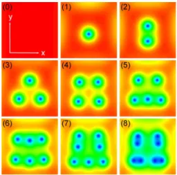
Figure2shows the contour plots of the magnitude of the order parameter兩⌿兩 for the final steady states in the sequence of branches at ␥= 0.4 as seen in Fig. 1. Increasing the field leads to an increase in the vortex number one by one. It is important to emphasize that this behavior is in sharp contrast

to that obtained in samples without current, where a single-vortex entry is prohibited. It has been extensively demon-strated that in a large system the vortices tend to form a triangular Abrikosov lattice. This scenario can change dra-matically in small samples where the boundary effects con-fine the equilibrium vortex configurations.6,29_Figure2shows

that a more complex vortex configuration can be obtained by combining a mesoscopic sample with an external bias cur-rent.

In Fig.3, we show a series of snapshots of both the mag-nitude and the phase of the order parameter for the current-driven vortices in the square sample. In Fig.3共a兲and1, three vortices form a triangular lattice with an axial symmetrical structure along y axis. Because of the Lorentz force induced by the applied current, vortices move slowly toward the negative y direction. In Fig.3共b兲 and1, a new vortex enters the sample and runs into the upper vortex of the triangle. This collision results from the fact that the central vortex moves slower than the new intruded one as a consequence of the vortex-vortex interaction. Figure 3共c兲and 1 shows that the incoming vortex collides with the central one and they merge into a giant vortex with L = 2. This remarkable coex-istence of a giant vortex with two satellite single-quantum ⌽0vortices below, forming a noncentral symmetric structure,

is different from other giant vortex matter obtained in meso-scopic samples without external current.9_{As it is shown in}

the next images 关Figs.3共d兲, 1, 3共e兲, and 1兴, this giant 2⌽₀

vortex is not stable and eventually splits in two ⌽₀vortices due to the strong repulsive interaction between them.

Figures 3共a兲, 2, 3, and 2 show the contour plots of the phase of the order parameter corresponding to the snapshots shown in Figs.3共a兲,1–3, and 1. An integration path around the superconductor shows that the phase changes 3⫻2␲ in Fig. 3共a兲 and 2 and 4⫻2␲ in Figs. 3共b兲, 2, 3, and 2. In addition, around isolated vortices, as seen in Figs. 3共a兲, 2,

3共b兲,2,3共d兲, and2, the phase changes by 2␲, whereas in Fig.

3共c兲and2it changes by 4␲around the central giant vortex. This result provides unambiguous and compelling evidence of the formation of a giant vortex state.

In order to understand the process of nucleation and an-nihilation of the giant vortex, we calculated the correspond-ing free energy, magnetization, and vorticity for the whole FIG. 2.共Color online兲 Contour plots of 兩␺兩 at ␥=0.4 for different

fields H/H_c2= 0, 0.38, 0.44, 0.45, 0.54, 0.65, 0.7, 0.76, and 0.85, respectively. The dots represent the vortex core positions in the system with low兩␺兩 value. The index numbers 共0兲–共8兲 in each plot also present the total vorticity L in the system.

FIG. 3. 共Color online兲 共a1兲–共e1兲 and 共a2兲–共e2兲 are contour plots of the distribution of the magnitude of the order parameter 兩␺兩 and their corresponding phase␸ at H/H_c2= 0.5 with the applied current density␥=0.8 along x direction at different time: 共a1兲 and 共a2兲: 77.76; 共b1兲 and共b2兲: 86.04; 共c1兲 and 共c2兲: 95.688; 共d1兲 and 共d2兲: 98.28; and 共e1兲 and 共e2兲: 104.4. The arrows illustrate the direction and the speed of the vortex motion.

system as a function of time. The results are summarized in Fig. 4共a兲. The free energy exhibits a series of cusps as a function of time each of which corresponding to a change in vorticity in the system. Furthermore, the magnetization curve is in agreement with the vorticities of the superconducting system, which represents the diamagnetic variation in the sample.

At the point a in Fig.4共a兲, the magnetic signal increases rapidly and the free energy reaches a local maximum corre-sponding to the nucleation of a new vortex in the boundary region 关Fig.3共a兲 and1兴. After the entrance of the new

in-coming vortex, the whole system composed by the four vor-tices undergoes a relaxation process reflected in the decrease in the free energy till point b. Later on, as anticipated in Figs.

3共c兲,1,3共c兲, and2, two⌽0vortices collide and merge into a

giant vortex at point c. This event manifests itself as an in-crease in the free energy after point b and a kink structure around points c and d as seen in Fig.4共a兲. After this, the free energy continues to increase and reaches a peak value corre-sponding to the sharp drop of the magnetization at t⬇112, where two vortices are removed from the sample by the ap-plied current.

In general, the process of vortex collision and formation of a giant vortex is difficult to identify in the free energy.

This is due to its small contribution to the total energy which is dominated by the self-energy of the vortices. The global free-energy maximum or the saddle point always indicates a change in the vortex number during the vortex flow in the sample. Since the collision process happens in the nonequi-librium vortex flow state, the signal response of the evolution of the collision process is always smaller than that of the vortex nucleation or vortex annihilation at the edges in the contribution of the global free energy as seen in Fig. 4共a兲. Therefore, from the global free energy is hard to disclose the vortex-collision process as well as the nucleation and the annihilation of the giant vortex in the multivortex system with changeable vorticities. Additionally, since the total vor-ticity of the system retains L = 4 from t⬇78 to 112, the pro-cess of nucleation and annihilation of the giant vortex shows no features in the magnetization curve. In order to under-stand the transition between the giant vortex and the single-quantum vortices, in Fig.4共b兲, we show the evolution of the free-energy zooming in the time window where the process of giant vortex formation occurs. The calculation demon-strates clearly that the maximum free energy of the desig-nated area coincides with the giant vortex state. Therefore, we believe that the local free energy in the collision area by neglecting the irrelevant events in the whole system can properly characterize the nucleation and the annihilation pro-cess of the giant vortex transformation. We would like to mention that the dynamic origin of formation of a giant vor-tex is substantially different than the static case,9,29,31_where

the total vorticity can be revealed exactly by the free energy. We also want to point out that the vortex collision and the giant vortex always appear in a very short time scale in the nonequilibrium state in the perfect system. The possible way to extend the lifetime of the giant vortex is to introduce the pinning defect in the system, which may make it easier to observe the giant vortex matter experimentally.

In what follows, we will demonstrate that the formation of giant vortices becomes easier at high magnetic fields. In this limit, more ⌽0 vortices flow inside the sample at the same

time and the probability of vortex collision increases. In Figs. 5共a兲 and5共b兲, we show the contour plots of both the magnitude and the phase of the order parameter for the vor-tex dynamics in the current driven system at H/Hc2= 0.9.

One can see clearly the coexistence of single-quantized vor-tices and a giant vortex in the system. Interestingly, for high magnetic fields, giant vortices can bear more than two flux quanta. Additionally, we have carried out the simulations for different sample sizes and ␬ values to determine the rel-evance of these parameters in the formation of giant vortices. FIG. 4. 共Color online兲 共a兲 Time evolution of free-energy 共blue

curve兲, magnetization 共red curve兲, and vorticity 共magenta segment lines兲 of the square superconducting system with ␥=0.8 and H/Hc2= 0.5. The dashed vertical lines a–e guide the eyes for the evolution corresponding to the snapshots shown in Fig.3.共b兲 Time evolution of free energy in the designated patches with the same size for the process of the giant vortex formation. The insets show the snapshots at point b, c, and d, which have been framed in Figs. 3共b兲,1–3, and1.

FIG. 5. 共Color online兲 Contour plots of 共a兲 兩␺兩 and 共b兲 ␸ of the order parameter with H/Hc2= 0.9 and␥=0.8 at certain time in the simulation.

In a large square sample, we mostly obtain a moving lattice of single quantized⌽0vortices with the applied current. This

finding suggests that the limited size of the sample is the most crucial factor for the giant vortex formation, in similar fashion to the giant vortex formation in a system without current.9,29,31 We have also checked that the collision event and the subsequent giant vortex formation occurs in a wide range of␬values as long as the external magnetic field and the current density in the system are properly tuned.

IV. SUMMARY

We have studied numerically the current-driven vortex dynamics in a square mesoscopic superconductor by TDGL equations. We showed that the applied current can break the symmetry imposed by the sample geometry and significantly influence the vortex penetration and distribution in the sample. Our simulations show a series of asymmetric con-figurations of the vortex entries under the bias current, which are quite different from the symmetry distribution obtained without the current.29 _{Although the occurrence of a}

single-vortex entry in a symmetric square sample can be excited by the thermal fluctuation which is neglected here,14,15,29 _the

configuration and the directional flow of the vortex lattice inside the sample cannot be duplicated. In addition, we have

found clear giant vortex formation through a collision in-volving two individual vortices. Clear evolution of the vortex configurations for the nucleation and the annihilation of the giant vortex has been revealed when the system is exposed to the current. We propose that the local free energy character-izes well the process of the nucleation and annihilation of the giant vortex. We also want to emphasize that the surface barrier plays a crucial role for the giant vortex formation in the collision process, which not only accelerates the new born vortex to rush into the central area but also decelerates or even stops the vortex to escape from the sample due to the driving current. Our study reveals a method for the giant vortex formation in the mesoscopic superconductor and it is beneficial for the design of the current-driven vortex device based on the microstructured superconductors, such as the quantum-fluxon rectifiers, vortex pumps, diodes, or lenses.32

ACKNOWLEDGMENTS

We acknowledge the support from the MOST, NSF, SRF for ROCS, SEM, and the BIL Flanders-China Projects of China. This work was also supported by Methusalem Fund-ing of the Flemish government, FWO-Vlaanderen, and the Belgian Inter-University Attraction Poles IAP Programmes. A.V.S. is grateful for the support from the FWO-Vlaanderen.

1_{A. I. Buzdin and J. P. Brison, Phys. Lett. A 196, 267共1994兲.} 2_{J. J. Palacios, Phys. Rev. B 58, R5948共1998兲.}

3_{A. K. Geim, I. V. Grigorieva, S. V. Dubonos, J. G. S. Lok, J. C.}

Maan, A. E. Filippov, and F. M. Peeters, Nature共London兲 390, 259共1997兲.

4_{B. J. Baelus, L. R. E. Cabral, and F. M. Peeters, Phys. Rev. B 69,}

064506共2004兲.

5_{H. J. Zhao, V. R. Misko, F. M. Peeters, V. Oboznov, S. V.}

Du-bonos, and I. V. Grigorieva, Phys. Rev. B 78, 104517共2008兲; V. R. Misko, B. Xu, and F. M. Peeters, ibid. 76, 024516共2007兲; V. R. Misko and F. M. Peeters, ibid. 74, 174507共2006兲.

6_{L. F. Chibotaru, A. Ceulemans, V. Bruyndoncx, and V. V.}

Mosh-chalkov, Nature共London兲 408, 833 共2000兲; Phys. Rev. Lett. 86, 1323共2001兲; V. R. Misko, V. M. Fomin, J. T. Devreese, and V. V. Moshchalkov, ibid. 90, 147003共2003兲.

7_{B. J. Baelus, A. Kanda, N. Shimizu, K. Tadano, Y. Ootuka, K.}

Kadowaki, and F. M. Peeters, Phys. Rev. B 73, 024514共2006兲; B. J. Baelus, A. Kanda, F. M. Peeters, Y. Ootuka, and K. Kad-owaki, ibid. 71, 140502共R兲 共2005兲; A. K. Geim, S. V. Dubonos, J. J. Palacios, I. V. Grigorieva, M. Henini, and J. J. Schermer, Phys. Rev. Lett. 85, 1528共2000兲; P. S. Deo, V. A. Schweigert, F. M. Peeters, and A. K. Geim, ibid. 79, 4653共1997兲.

8_{A. Kanda, B. J. Baelus, F. M. Peeters, K. Kadowaki, and Y.}

Ootuka, Phys. Rev. Lett. 93, 257002共2004兲.

9_{B. J. Baelus and F. M. Peeters, Phys. Rev. B 65, 104515共2002兲.} 10_{V. A. Schweigert, F. M. Peeters, and P. S. Deo, Phys. Rev. Lett.}

81, 2783共1998兲.

11_{E. Sardella, A. L. Malvezzi, P. N. Lisboa-Filho, and W. A. Ortiz,}

Phys. Rev. B 74, 014512共2006兲.

12_{V. Bruyndoncx, J. G. Rodrigo, T. Puig, L. Van Look, V. V.}

Mosh-chalkov, and R. Jonckheere, Phys. Rev. B 60, 4285共1999兲.

13_{I. V. Grigorieva, W. Escoffier, V. R. Misko, B. J. Baelus, F. M.}

Peeters, L. Y. Vinnikov, and S. V. Dubonos, Phys. Rev. Lett. 99, 147003共2007兲.

14_{T. Nishio, S. Okayasu, J. Suzuki, and K. Kadowaki, Physica C}

379, 412共2004兲.

15_{S. Okayasu, T. Nishio, Y. Hata, J. Suzuki, I. Kakeya, K.}

Kad-owaki, and V. V. Moshchalkov, IEEE Trans. Appl. Supercond. 15, 696共2005兲.

16_{N. Schildermans, A. Yu. Aladyshkin, A. V. Silhanek, J. Van de}

Vondel, and V. V. Moshchalkov, Phys. Rev. B 77, 214519 共2008兲.

17_{M. Morelle, V. Bruyndoncx, R. Jonckheere, and V. V.}

Mosh-chalkov, Phys. Rev. B 64, 064516共2001兲.

18_{C. R. Hu and R. S. Thompson, Phys. Rev. B 6, 110共1972兲.} 19_{T. Winiecki and C. S. Adams, J. Comput. Phys. 179, 127共2002兲.} 20_{M. Machida and H. Kaburaki, Phys. Rev. Lett. 71, 3206共1993兲.} 21_{D. Y. Vodolazov and F. M. Peeters, Phys. Rev. B 76, 014521}

共2007兲.

22_{R. Kato, Y. Enomoto, and S. Maekawa, Phys. Rev. B 44, 6916}

共1991兲; 47, 8016 共1993兲.

23_{Q. Du, M. D. Gunzburger, and J. S. Peterson, SIAM Rev. 34, 54}

共1992兲; Q. Du, Contemp. Math. 329, 105 共2003兲.

24_{W. D. Gropp, H. G. Kaper, G. L. Leaf, D. M. Levine, M.}

Palumbo, and V. M. Vinokur, J. Comput. Phys. 123, 254共1996兲.

25_{P. G. de Gennes, Superconductivity of Metals and Alloys}

共Adison-Wesley, New York, 1989兲.

26_{A. D. Hernández and D. Domínguez, Phys. Rev. B 65, 144529}

共2002兲.

Nauk 163, 105共1993兲.

28_{M. Tinkham, Introduction to Superconductivity 共Dover, New}

York, 2004兲.

29_{S. Kim, C.-R. Hu, and M. J. Andrews, Phys. Rev. B 69, 094521}

共2004兲.

30_{M. Morelle, J. Bekaert, and V. V. Moshchalkov, Phys. Rev. B}

70, 094503共2004兲.

31_{D. S. Golubović, M. V. Milosević, F. M. Peeters, and V. V.}

Moshchalkov, Phys. Rev. B 71 180502共R兲 共2005兲.

32_{B. Y. Zhu, F. Marchesoni, V. V. Moshchalkov, and F. Nori, Phys.}

Rev. B 68, 014514 共2003兲; B. Y. Zhu, F. Marchesoni, and F. Nori, Phys. Rev. Lett. 92, 180602共2004兲.