Coupling between flow and sediment deposition in rectangular shallow reservoirs

Coupling between flow and sediment deposition in rectangular

shallow reservoirs

ERICA CAMNASIO (IAHR Member), Researcher, Department of Civil Engineering and Architecture (D.I.C.Ar.), Università di Pavia, via Ferrata, 3, 27100 Pavia, Italy.

Email: erica.camnasio@unipv.it

SEBASTIEN ERPICUM (IAHR Member), Laboratory Manager, ArGEnCo Department, Research group Hydraulics in Environmental and Civil Engineering (HECE), University of Liege (ULg), Chemin des Chevreuils, 1, bat B52/3, étage +1, 4000 Liège, Belgium.

Email: s.erpicum@ulg.ac.be

ENRICO ORSI (IAHR Member), Professor, Department of Hydraulic, Environmental, Infrastructures and Surveying Engineering (D.I.I.A.R.), Politecnico di Milano (POLIMI), Piazza Leonardo da Vinci 32, 20133 Milano, Italy.

Email: enrico.orsi@polimi.it

MICHEL PIROTTON (IAHR Member), Professor, ArGEnCo Department, Research group Hydraulics in Environmental and Civil Engineering (HECE), University of Liege (ULg), Chemin des Chevreuils, 1, bat B52/3, étage +1, 4000 Liège, Belgium.

Email: michel.pirotton@ulg.ac.be

ANTON J. SCHLEISS (IAHR Member), Professor, Laboratory of Hydraulic Constructions (LCH), Ecole Polytechnique Fédérale de Lausanne (EPFL), Station 18, 1015 Lausanne, Switzerland.

Email: anton.schleiss@epfl.ch

BENJAMIN DEWALS (IAHR Member), Assistant Professor, ArGEnCo Department, Research group Hydraulics in Environmental and Civil Engineering (HECE), University of Liege (ULg), Chemin des Chevreuils, 1, bat B52/3, étage +1, 4000 Liège, Belgium.

Coupling between flow and sediment deposition in rectangular shallow

reservoirs

ABSTRACT

Flow velocity and sedimentation patterns were investigated experimentally and numerically in shallow rectangular reservoirs with different asymmetric locations of the inlet and outlet channels. Velocity fields were measured in the entire reservoir, both for clear water flow and with suspended sediments. Thickness of sediment deposits were mapped in the whole reservoir by means of a laser light method. In one of the studied geometric configurations, injection of suspended sediments led to a complete change in the observed flow field. Experimental results were compared with numerical simulations performed with the depth-averaged flow model WOLF 2D, using a depth-averaged k- turbulence model. The simulations lead to accurate predictions of the velocity profiles and the change in flow pattern as a result of sediment deposits was successfully reproduced.

Keywords: flow stability, morphodynamic evolution, numerical modelling, reservoir sedimentation, shallow reservoir

1. Introduction

Shallow rectangular reservoirs are common engineering structures in urban and fluvial hydraulics. Sediment deposition in these structures must be either minimized or maximized, depending on whether the reservoirs are used as storage basin or settling tank. Consequently, optimal design, operation and maintenance of shallow reservoirs should be based on accurate predictions of trapping efficiency and location of sediment deposits, which highly depend on the flow features in the reservoir.

According to recent research, complex flow fields with large scale horizontal vortices develop in such reservoirs despite their simple geometry (Dewals et al. 2008, Dufresne et al. 2010a, Camnasio et al. 2011). In addition to symmetric jet flows, several asymmetric flow patterns were indeed observed in spite of the hydraulic and geometric symmetry of the setup. They are characterized by the presence of one or two stagnation points on the side-walls. In addition, bi-stable flow fields were observed and suspended load or sediment deposits may cause a feedback effect on the flow pattern itself, as already shown by Kantoush (2008) and further analysed here.

Several authors have shown that existing empirical relationships for the estimation of reservoir trapping efficiency often fail to deliver accurate predictions because they do not consider explicitly the influence of the type of flow pattern on sediment deposition (Dufresne et al. 2010b, Kantoush 2008, Stovin 1996, Saul and Ellis 1992). More knowledge is therefore

necessary to clarify the relationships between the reservoir geometry, the type of flow pattern and the amount of deposits.

In this respect, Stovin (1996) experimentally and numerically analysed the influence of several physical parameters on the efficiency of storage chambers, including the flow rate, the length-to-width ratio of the reservoir, the longitudinal slope and the benching gradient. Stovin (1996) concluded that the pattern of sediment deposits is strongly influenced by the distribution of bed shear stress, highlighting thus the need for accurately predicting the flow field.

Experiments with suspended load were also carried out by Kantoush (2008), who investigated reservoir geometries characterized by a symmetrical location of the inlet and outlet channels but with varying reservoir length and width. The pattern of sediment deposition was measured using an echo-sounder and empirical relationships were developed to predict the influence of reservoir geometry on the trapping efficiency. Kantoush (2008) observed several examples of changes of the flow field when the thickness of sediment deposits exceeded about 0.15 times the water depth.

While the tests performed by Kantoush (2008) were based on high concentrations of fine sediments, a complementary experimental campaign was undertaken at the University of Liege (ULg) with bed load and sediment inflows lower than the transport capacity of the flow at the inlet (Dufresne et al. 2010b, Dufresne et al. 2012). Since these experiments focused on the short term deposition pattern in the reservoir, their duration was too short to lead to a feedback of deposits on the flow pattern.

Numerical simulations of flow in rectangular shallow reservoirs mainly focused on low and moderate Reynolds numbers, for which symmetry of the flow may be broken as the Reynolds number increases. Mizushima and Shiotani (2001) and Mullin et al. (2003) focused on Reynolds numbers Rb below 1,500 (Rb = Vin b / 2 / , with Vin the inlet velocity, b the width of the inlet channel and  the kinematic viscosity of water). Some attempts were also undertaken to predict flow fields and deposition patterns for turbulent free surface flows in rectangular shallow reservoirs (Rin = Vin 4 h /  > 10

5

, with h the water depth). Among others, Adamsson et al. (2003) tested different boundary conditions at the reservoir bottom to reproduce the deposition pattern in storage tanks using the commercial model FLUENT. They showed that a bottom boundary condition based on the critical bed shear stress performed better than other approaches, which either did not allow particles to become resuspended into the flow after first contact with the bottom, or were not directly related to flow characteristics and physical properties of the sediments.

Persson (2000) performed 2D numerical simulations with the commercial software Mike21 to analyse the flow field in reservoirs of different geometries, including

configurations with baffles or an island in the reservoir. Based on the comparison of residence time distribution functions of a tracer instantaneously injected at the inlet, the results confirmed that the length-to-width ratio and the location of inlet and outlet have a large impact on the hydraulic performance of the reservoir (Persson 2000, Persson et al. 1999, Persson and Wittgren 2003).

By introducing a disturbance in the inlet velocity profile, Dewals et al. (2008) successfully simulated bifurcating flows in rectangular shallow reservoirs, whereas Dufresne (2008) used a disturbance in the initial condition to reproduce similar symmetric and asymmetric flows. Dufresne et al. (2011) combined both approaches and simulated bi-stable flow fields in reservoirs of intermediate length, whereas shorter reservoirs lead to a symmetric flow and longer ones to an asymmetric flow pattern. The existence of such bi-stable flow fields was also highlighted by Dewals et al. (2012).

Recently, Peng et al. (2012) applied a lattice Boltzmann model to the configurations previously modelled by Dewals et al. (2008) and achieved a similar level of accuracy as Dewals et al. (2008).

Although some asymmetric reservoir configurations were considered by Persson (2000), no detailed analysis of the influence of inlet and outlet channel positioning was carried out so far. Therefore, the objective of this paper is to investigate how different locations of inlet and outlet channels may influence the flow field, the location of sediment deposits and possible feedback effects on the flow. To this end, we reanalyse here one reservoir configuration previously studied by Camnasio et al. (2011) and we extend their analysis by considering inlet and outlet channels located not only along the centreline of the reservoir, but also in different asymmetric configurations.

We first present the results of experimental tests conducted for four geometric configurations of the inlet and outlet channels. The experiments were carried out with clear water and with an inflowing suspended load. In one of the considered geometric configurations, a significant change in the flow field was observed as suspended sediments were injected. To provide more insight into this effect, flow simulations were performed using the depth-averaged flow model of Dewals et al. (2008) and also used by Dufresne et al. (2011). Although no morphodynamic simulations were conducted, the effect of sedimentation has been incorporated into the flow simulations based on a time-dependent topography of the bottom of the reservoir, representing the gradual development of experimentally measured sediment deposits.

2. Experimental set up

Polytechnique Fédérale de Lausanne (EPFL), in the same facility as used by Dewals et al. (2008) and Camnasio et al. (2011).

2.1. Shallow reservoir facility

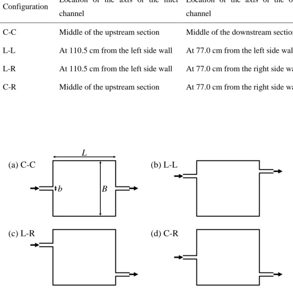
The experimental setup is a rectangular shallow PVC reservoir with a smooth flat bottom (maximum depth 0.3 m, maximum length 6 m and maximum width 4 m) endowed with inlet and outlet free surface channels (width b = 0.25 m, length 1 m each) having the same depth as the reservoir. The channels can be moved respectively along the upstream and the downstream side of the reservoir in order to obtain reservoir configurations with asymmetric locations of the inlet and outlet channels. The four configurations considered in the present work are sketched in Fig. 1 and referred to, respectively, as C-C, L-L, L-R and C-R as defined in Table 1.

Movable PVC walls enable the length L and the width B of the reservoir to be adjusted in order to test different length-to-width ratios L/B and expansion ratios B/b. For the tests presented here, the reservoir width was set to B = 4 m and the reservoir length to L = 4.5 m. This configuration was considered previously by Camnasio et al. (2011) and has been selected here as a reference because, for a central location of the inlet and outlet channels (C-C), it leads simply to a stable symmetric flow field, involving a straight jet from the inlet to the outlet and one recirculation developing on each side of the main jet.

The reservoir is fed with a constant discharge Q and the water depth h is regulated by a flap gate placed at the end of the outlet channel. The inflow discharge is measured by an electromagnetic flow meter. A second discharge check is obtained by water level measurement above the flap gate in the outlet channel. A honeycomb in the inlet enables an almost uniform velocity distribution across the channel cross section to be obtained.

2.2. Flow and sediment characteristics

In the present experiments, the water depth was fixed at h = 0.2 m for a constant discharge of Q = 7 l/s. The resulting Froude and Reynolds numbers in the inlet channel are Fin = Q/(bgh3/2) = 0.1 and Rin = Vin 4 h /  = 112,000.

Since the primary goal of the paper is focused on the influence of the reservoir geometry (location of inlet and outlet channels) and not on the influence of different sediment inflows, the same sediment characteristics and inlet concentration as considered previously by Dewals et al. (2008) and Kantoush (2008) were selected in the present experiments.

These sediments consist in crushed walnut shells. They are characterized by a solid particle density s = 1500 kg/m

3

, determined by pyknometry, an average diameter dm = 112 m, a median diameter d50 = 89 m and a coefficient of uniformity d60/d10 = 4.

During the tests, the sediments were continuously fed from a container into a mixing tank, where they were mixed to the inflowing discharge by a rotating propeller. The mean inflowing concentration Cin was about 2 g/l, corresponding to 200 kg of sediments supplied to the tank during four hours of experiment (sediment discharge Qs = 0.014 kg/s; average volumetric concentration = 0.13%).

According to the criterion of Bagnold (1966), about 75% of the grain size distribution can be carried by the flow as suspended load, since the ratio between the friction velocity U* (~ 0.005 m/s) and their settling velocity vss exceeds unity. Nevertheless, the inflowing suspended load Qs was about one order of magnitude higher than the transport capacity in the inlet channel (average volumetric concentration ~ 0.13%), as evaluated for the different size fractions by applying the formula of Celik and Rodi (1991). As a consequence, sediment deposits were also observed in the inlet channel.

The geometric and hydraulic conditions of the experiments were initially designed to schematize a real shallow reservoir located along river Rhone in Switzerland, in which sedimentation should be minimized as it is used to store river flood flows (Bollaert et al., 2000; Kantoush et al., 2005). The geometric scale was 1:50 and Froude similarity was applied. The sediment grain size in the model was chosen to scale properly the settling velocity. It corresponds to fine sand in the field, with a mean diameter of 0.13 mm. The sediment supply rate in the model was selected to keep approximately the same volumetric concentration as in the field (0.14%). This value corresponds to 3.6 g/l, which is an upper bound of the range of measured concentrations in river Rhone during flood conditions upstream of Lake Geneva.

2.3. Measurement of velocity fields

Since the turbulent coherent structures characterizing the flow field consist mainly in large horizontal eddies with a vertical axis, velocity measurements were focused on the horizontal components of the velocity. By means of a limited number of purpose-made measurements, the average vertical velocity component was shown to remain two orders of magnitude lower than the characteristic horizontal velocity Q/(bh) and may thus be neglected (shallow flow assumption).

Eight UVP transducers (Metflow, 2002), mounted on a movable square grid, were used to measure the horizontal velocity component along the axis of each transducer and up to a distance of 723 mm. At the 16 intersections between the velocity profiles recorded by each transducer, instantaneous horizontal velocity vectors were obtained and averaged over 150 successive records. By moving the grid to 16 different positions, the whole surface of the 4.5 m × 4 m reservoir could be covered, enabling to depict the average horizontal velocity

field throughout the reservoir (Camnasio et al. 2011). The transducers were placed at a height of 0.4 h = 8 cm from the reservoir bottom, where velocity corresponds to the average value if a vertical logarithmic velocity profile is assumed. Specific velocity measurements performed at different levels in the flow confirmed the logarithmic velocity profile. From the measured velocity profiles, the friction velocity was estimated at approximately 0.005 m/s.

2.4. Measurement of sediment concentration and deposits

During the whole experiments, sediment concentration was continuously monitored by two turbidity-meters (SOLITAXsc100, 2005), respectively placed in the inlet and outlet channels. A calibration curve was used to convert the optical measurement of turbidity into the corresponding sediment concentration C (g/l). Surrounding light, flow turbulence and the vicinity of side-walls had no significant influence on the calibration curve. The inflowing and outflowing sediment concentrations were also monitored by water sampling during the experiments.

The thickness of sediment deposits on the entire reservoir bottom was measured by a laser technique (Baumer, OADM13), after two hours and after four hours of sediment supplying. The laser was placed in a water-proof box attached to a movable metal bar at a known height from the reservoir bottom. A linear relationship has been calibrated in real operating conditions to relate the voltage supplied by the laser instrument to the distance of the laser light source to the top of the sediment deposits, from which the thickness of sediment deposits can be derived. The measurements were performed on a regular grid covering the entire reservoir bottom by steps of 50 cm. More detailed measurements were additionally taken along the axis of the inlet and the outlet channels.

3. Numerical model

Flow modelling was performed with the academic code WOLF 2D developed at the University of Liege. A detailed description of the model was provided by Dewals et al. (2008), who already used and validated the model for the same experimental setup as considered here.

The model solves the shallow-water equations using multiblock Cartesian grids and a second-order accurate finite volume scheme. The fluxes are computed by a self-developed flux vector splitting, which is Froude-independent and well-balanced with respect to the pressure and bottom slope terms (Erpicum et al., 2010a). The turbulent fluxes are evaluated by means of a centred scheme. The time integration is performed by means of a 3-step Runge-Kutta algorithm and a semi-implicit treatment of the bottom friction term is used. The time

step is adaptive and computed based on the Courant-Friedrichs-Lewy (CFL) stability criterion, with a CFL number equal to 0.5. It takes values of the order of 8 × 10-3 s.

This finite volume model has already proven its validity and efficiency for the analysis of flow in shallow reservoirs (Dewals et al., 2008; Dufresne et al., 2011) as well as numerous other applications including complex turbulent flows (Erpicum et al., 2009; Roger et al., 2009) and geophysical flows (Dewals et al. 2011; Ernst et al., 2010; Erpicum et al., 2010b).

For all simulations in this study, unsteady computations were performed until a steady-state was reached. The grid spacing was set to 0.025 m. A grid independence test is presented in Dufresne et al. (2011), based on the grid convergence index proposed by Roache (1994).

Most simulations were conducted assuming a smooth bottom and smooth side-walls. However, to analyse the influence of an increased bottom roughness induced by the deposits, flow simulations were also performed considering different roughness heights ks, ranging between 0.000 m and 0.005 m. This range covers grain roughness effects (d50 - d90 ≈ 89 – 215 × 10-6 m) and 0.005 m is an upper bound of bed form heights observed on the reservoir bottom. Although smooth walls are obviously characterized by a non-zero value of ks,

ks = 0.000 m was considered here as a lower bound of the range of variation of ks and, as such, was also used in the simulations. The corresponding friction coefficient cf has been evaluated using Colebrook formula for open channel flows (Chanson, 1999):

10

1

2.52

2 log

14.83

4

4

k

h

c

c









 









R



It ranges between 4.4 × 10-3 (smooth bottom) and 8.3 × 10-3 (ks = 5 × 10 -3

m). The corresponding bed friction number S = cf ( B – b ) / ( 4 h ), as defined by Babarutsi et al. (1989), ranges from 0.02 to 0.04 and corresponds thus to non-frictional flow conditions. For wall roughness, the same formulation as in Dewals et al. (2008) is used.

Several types of turbulence models exist, ranging from simple algebraic expressions of the eddy viscosity (Fischer et al., 1979; Wark et al., 1990) to more advanced models with several additional transport equations (e.g., Rodi, 1984). In this study, the eddy viscosity was evaluated based on a depth-averaged k- model with two different length-scales accounting for vertical and horizontal turbulence mixing, as described by Babarutsi and Chu (1998) or Erpicum et al. (2009). The model considers separately the large-scale transverse-shear-generated turbulence, associated to the horizontal length-scale of the flow, and the small-scale bed-generated turbulence having a characteristic dimension in the order of magnitude of the

water depth. This assumes that large scale velocity fluctuations are confined in the main flow plane, whereas the small scale fluctuations are three-dimensional (Babarutsi and Chu, 1998).

The turbulence model was derived following a two-step Reynolds averaging procedure. The first step filters out the bed-generated turbulence by treating the small scale fluctuations of the instantaneous 3D velocity components with an algebraic model. The second one considers the transverse-shear-generated turbulence by means of additional fluctuations of the depth-averaged velocity components in the main flow plane, modelled by two additional transport equations: one for the depth-averaged turbulent kinetic energy, and one for the depth-averaged turbulence dissipation rate. As proposed by Babarutsi and Chu (1998) and Erpicum et al. (2009), the calculations were performed using a set of coefficients assumed the same as for unconfined three-dimensional flow.

Consistently with the procedure described by Dewals et al. (2008), a slightly disturbed velocity profile was used as inflow boundary condition in all simulations, in order to introduce a seed for asymmetry. This approach is necessary to evaluate the stability of symmetric flow fields computed in the C-C configuration. The disturbance varies linearly between – 1% to + 1% along the cross-section of the inlet channel. Simulations with disturbances of different magnitudes (1% to 5%) were also tested. They confirmed that such small disturbances act only as a seed for asymmetry, since the final computed result is not significantly affected by the magnitude of the disturbance. In order to control the velocity profile exactly at the inlet of the reservoir, this boundary condition was prescribed at the reservoir boundary (i.e., downstream of the inlet channel).

In all simulations, the free surface elevation was prescribed as boundary condition downstream of the outlet channel; except in simulations starting from an empty reservoir, for which a stage-discharge relationship was prescribed at the same location, reproducing the overflow over the flap gate in the experimental setup. In these simulations, wetting and drying of cells is handled free of mass conservation error thanks to a specific iterative procedure (Erpicum et al., 2010b; Roger et al., 2009). A grid adaptation technique restricts the computation domain to the wet cells.

4. Experimental results

4.1. Velocity fields

Velocities were first measured during clear water tests, then during tests with sediment supply, in order to investigate the possible influence of sediment deposits and/or of suspended load on the flow pattern. Vector velocity maps were produced for all the tested reservoir configurations, showing that in all tested configurations velocities along the main jet were in

the range of 100-120 mm/s (± 5 %), while in the centre of the recirculation zones, the velocity reaches a minimum of about 10-20 mm/s (± 5 %).

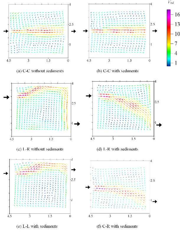
The time-averaged horizontal velocity, V, measured at 0.4 × h, was normalized by the plug flow velocity Vres = Q/(B·h) = 8.75 mm/s (Oca et al., 2004). The distributions of the normalized velocity Vnd = V / Vres are shown in Fig. 2 for the clear-water tests and for the tests with suspended sediments. Only in the L-R configuration, the flow pattern observed with suspended sediments differs significantly from the flow pattern with clear water.

In the C-C configuration, a large eddy is observed on both sides of the main jet and, on the right side of the jet, a second smaller eddy can also be seen. This flow field corresponds to a transition between a flow pattern with four eddies (referred to as “S1” in Camnasio et al. 2011) and a flow pattern characterized by only one large eddy on each side of the jet (“S0” in Dufresne et al. 2010a), which develops if L / B ≤ 1 according to Camnasio et al. (2011). A local increase of the velocity in the main jet can be seen in Fig. 2(b), due to the shape of sediment deposits, as detailed in section 4.2.

In the L-L configuration, the main jet is deflected towards the closer side wall, where it reattaches and follows the wall until it reaches the outlet channel, as shown in Fig. 2(e). A large re-circulation zone develops in the remaining part of the reservoir. The deflection of the jet towards the lateral wall may be attributed to the “Coanda effect” (Wille and Fernholz, 1965). Other examples of such deviation of a free surface water jet towards a lateral wall can be found in Lalli et al. (2004), Dewals et al. (2008) or Dufresne et al. (2010a).

In the L-R configuration, a flow field with one reattachment point on the left side wall was obtained in the tests without sediments, as shown in Fig. 2(c). The main jet is deflected towards the closer lateral wall, where it reattaches and follows the wall until the outlet. In contrast, Fig. 2(d) shows that a jet without reattachment point was observed in the tests with sediments. This change in flow pattern occurred after only about 30 min of sediments supply, when the maximum thickness of sediment deposits was 3 to 4 mm. Afterwards, the flow pattern remained stable during the remaining duration of the experiment.

The flow field observed in the clear-water test appears thus relatively unstable, as it has been completely modified by a relatively small perturbation, namely the supply of suspended sediments. The numerical simulations discussed in section 5 aim at giving more insight into the possible mechanism leading to such a change in flow pattern.

In the intermediate configuration C-R (Fig. 2f), the jet reaches the outlet without reattachment on the side walls, nor impinging on the downstream wall as in the L-R configuration with suspended sediments. Two eddies of different sizes develop on both sides of the main jet.

4.2. Sediment deposits

Figure 3 presents maps of sediment deposits thickness recorded by the laser technique after 4 hours of sediment supplying. The thickness of deposits s has been normalized with respect to the water depth h.

In all configurations, the highest thickness of deposits is located along the path of the main jet, as can be noticed by comparing the deposit maps (Fig. 3) with the velocity maps (Fig. 2). This results from the high sediment supply rate at the inflow compared to the transport capacity of the flow.

The location of extremes in the pattern of deposits, similar to bed forms, coincides with the extremes in the velocity fields recorded by UVP after 4 hours of experiment and displayed in Fig. 2.

The maximum height of sediment deposits reaches about 40 mm along the path of the main jet, while sediment thickness in the centre of the recirculation zones remains lower than 5 mm, confirming that turbulent mixing drives only a small fraction of the sediments into the recirculation zones and that most of them settle down before reaching the core of the eddies.

These results differ from those carried out by Stovin and Saul (1994) or Dufresne et al. (2011), in which the sediment supply rate did not exceed the transport capacity of the flow in the main jet and, therefore, the sediments settled mostly in the core of the eddies where velocity and bed shear stress were minimum.

5. Numerical results and discussion

The numerical model has first been used to reproduce the measured steady flow fields. Next, detailed comparisons of measured and computed velocity profiles are presented. Finally, the time-evolution of the flow field in the reservoir has been computed with a forced evolution of the reservoir bathymetry according to the measurements of deposits thickness. The influence of bottom and wall roughness has also been analysed.

5.1. Flow patterns

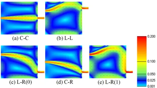
For the four tested reservoir geometries, Fig. 4 shows the flow fields simulated on a smooth and flat bottom with the k- turbulence model.

In the C-C configuration (Fig. 4a), the computed flow field is characterized by a straight jet with eddies on both sides, which is consistent with the experimental observations. The flow field remains essentially symmetric in spite of the seed for non-symmetry introduced through the inflow velocity profile. In the L-L configuration (Fig. 4b), the computed flow field is also in agreement with the experiments, in which one reattachment point was observed on the left side-wall.

In contrast, in the L-R configuration (Fig. 4c), the computed flow field does not match the experimental one. The former shows no reattachment point, whereas one reattachment point on the left side-wall was observed in the experiments with clear-water (Fig. 2c). The computed results compare actually better with the observations during tests with sediment supply (Fig. 2d). For the C-R configuration, the model predicts correctly a jet reaching directly the outlet without reattachment (Fig. 4d).

We investigated whether changing the initial condition of the numerical simulations may lead to a more satisfactory agreement between computed and measured flow fields in the L-R configuration. All simulations above were conducted based on an initial condition corresponding to a reservoir with 0.2 m water at rest. We show here that the initial condition influences the steady flow pattern obtained at the end of the simulation.

For the L-R configuration, the simulations were repeated starting from two different initial conditions, which lead to the following findings:

 when the simulations are performed starting from an empty reservoir, the k- model still leads to a flow pattern L-R(0);

 in contrast, when a steady flow pattern with lateral reattachment is used as initial condition (e.g., the flow field obtained in the L-L configuration, as shown in Fig. 4(b)), a flow pattern with jet reattachment is preserved at the end of the computation (Fig. 4e).

This demonstrates that both types of flow patterns, with and without lateral reattachment, are mathematical solutions of the system. It also suggests that the experimentally observed flow pattern may depend on the flow history, i.e. on the detailed experimental procedure. Another example of dependence of the flow pattern on the initial conditions was discussed by Dewals et al. (2012).

The same procedure was repeated for the C-C, L-L and C-R configurations, and the same flow patterns as shown in Fig. 4(a, b, d) were systematically obtained. This shows that the numerical predictions are robust for these three geometries and do not depend on the initial conditions.

5.2. Velocity profiles

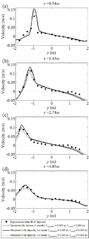
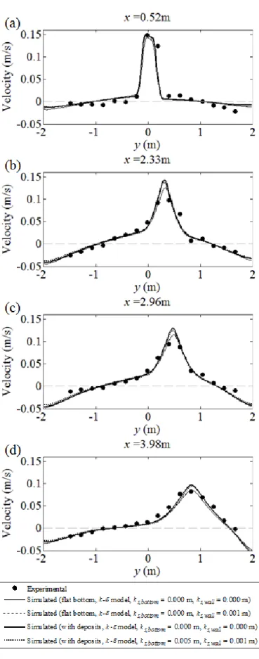
Figures 5 to 8 show profiles of the longitudinal velocity in different cross-sections of the reservoir. The influence of the bottom bathymetry as well as bottom and wall roughness is analysed.

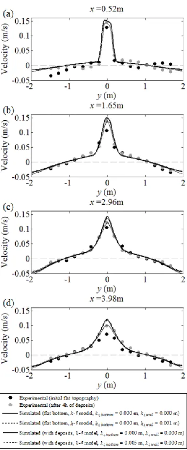
In the C-C configuration with a flat bottom (Fig. 5), the velocity profiles confirm that the numerical results follow closely the experimental observations in the recirculations. Only in

the centre of the jet, the computed velocity is higher than the measurements in most cross-sections, while it remains very accurate close to the inlet section (x = 0.52 m). No significant difference can be detected between the simulations with and without wall roughness.

When the topography corresponding to sediment deposits is considered, the velocity increases by about 20% in the centre of the jet and remains mostly unchanged in the lateral recirculations. Increasing the bottom roughness up to ks = 0.005 m leads to hardly noticeable changes in the velocity profiles. Flow resistance remains indeed very weak, since the head loss across the reservoir is in any case of the order of 1 - 2 × 10-4 m. These results are in agreement with Babarutsi et al. (1989 and 1991) and Chu (2004) for unilateral expansions: since the bed friction number remains here lower than 0.05, the flow is classified as “non-frictional” and is thus not influenced by the roughness.

In the L-L configuration (Fig. 6), the numerical predictions also lead to a satisfactory agreement with measurements. For all cross-sections, the bottom roughness hardly influences the velocity profiles.

In the L-R configuration (Fig. 7), for a flat reservoir bottom, the simulated flow field compares well with the experimental results. The wall roughness was varied between 0.000 m and 0.005 m, but no significant change in the velocity profiles could be detected. When the topography corresponding to the pattern of sediment deposits after 4 h is considered, the results of the k- simulation agree satisfactorily with the measurements. When bottom and wall roughness are included in the simulation, the velocity profiles change marginally.

In the C-R configuration (Fig. 8), a very good match is obtained between experimental data and the numerical results. Consistently with the other geometric configurations, bottom and wall roughness have little influence on the computed velocity field.

Since for all geometric configurations the simulation results were accurate to predict the velocity profiles, the model is considered as reliable to analyse the shift in flow pattern observed in the L-R configuration.

5.3. Change in flow pattern induced by sediment deposition

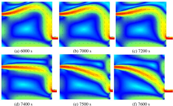
In the experiments, the flow pattern in the L-R configuration changed from one reattachment point on the left side wall to no reattachment point when suspended load was added to the flow. This change took place relatively quickly after the beginning of the experiment. To evaluate the capacity of the numerical model to reproduce this change in flow pattern, the time evolution of the measured thickness of sediment deposits has been implemented in the flow simulation as a time-varying topography. Four hours of flow have been simulated, corresponding to the total duration of the experiments with sediments. Since only three maps

of measured sediment deposits were available (initial condition, deposits after 2 h and deposits after 4 h), linear interpolation in time has been used for the intermediate time steps. At the end of the simulation, the mean thickness of deposits remains below 10% of the water depth.

After 4 hours of morphological evolution, no change in the computed flow patterns has been detected, except in the L-R configuration for which the simulated flow pattern changes from L-R(1) to L-R(0). This is consistent with the experimental results. In Fig. 9, the velocity magnitude in the middle of the reservoir is used as an indicator to appreciate the dynamics of the flow pattern modification. This variable confirms, for instance, that no macroscopic change in the flow pattern occurs in the C-R configuration, since a gradual rise in velocity can be observed (see secondary axis). In contrast, a sudden shift takes place in all simulations of the L-R configuration. The duration of this shift is of the order of 10 minutes, as depicted in detail in Fig. 10. Figure 9 reveals a strong influence of the bottom roughness on the timing of the change in flow pattern, as well as a moderate influence of the wall roughness. Interestingly, those two parameters did not influence significantly the velocity profiles (Fig. 7). Nonetheless, the timing of the change in flow pattern in the simulations (minimum 2 hours) remains higher than observed experimentally (about 30 min.). Consequently, the k- model succeeds in reproducing the process of flow pattern change for the right geometric configuration, but overestimates the time of change.

6. Conclusions

This paper analyses how the location of the inlet and outlet channels in rectangular reservoirs influences the velocity field and the sedimentation pattern in the reservoir. This issue is of high practical relevance, particularly in urban hydraulics, to optimize the design, operation and maintenance of man-made structures such as storm tanks or desilting basins.

Four geometric configurations have been considered, with the inlet and outlet channels located either along the centreline of the reservoir (C-C), both on the same side (L-L) or on opposite sides (L-R) of the centreline, or a combination of these (C-R). Experimental tests have been performed in a 4.5 m long and 4 m wide experimental reservoir, equipped with a system for continuous sediment supply. The velocity fields and the thickness of sediment deposits have been measured throughout the reservoir, respectively, by UVP transducers and a laser technique.

For the considered range of sediment supply rate, the position of the inlet and outlet channels (located on opposite sides of the reservoir) highly influenced the location of sediment deposits after 2 and 4 hours of tests, due to the very different flow fields developing in the different geometric configurations. In all configurations, the maximum thickness of

deposits was located along the main jet, because the sediment supply rate at the inflow was higher than the transport capacity of the flow in the main jet.

In one geometric configuration (L-R), the flow pattern completely changed once sediments were supplied: at the beginning of the tests, with clear water, the jet reattached on the left side-wall (pattern “L-R(1)”); whereas after about 30 min of sediment supply, a jet without reattachment point was observed (pattern “L-R(0)”). Afterwards, the flow pattern was stable during the remaining test duration. This is a case of two-way coupling between sediments and flow, since not only the flow governs sediment particles motion, but also sediments have a macroscopic effect on the flow.

The depth-averaged flow model WOLF 2D was applied to assess its ability to predict the flow patterns for the tested reservoir configurations. The gradual development of sediment deposits was reproduced in the flow simulations by means of a time varying topography based on measured thickness of sediment deposits.

Simulations with a two-length-scale k- turbulence model provided accurate predictions of the velocity profiles and they successfully reproduced the dynamic change in flow pattern from L-R(1) to L-R(0) as a result of the combined effect of bathymetry change and increased bottom roughness as a result of sediment deposits. While almost no influence of bottom and wall roughness could be detected on the computed steady velocity profiles, the roughness strongly influences the dynamics of the change in flow pattern. Although the timing of this change is still overestimated by the model, the process is well reproduced.

These results should be further confirmed using non uniform and time-dependent roughness distributions as well as more advanced turbulence modelling, such as large eddy simulations. The investigation of three-dimensional secondary currents would be of interest. Additional experimental tests enabling to directly measure the flow turbulence characteristics are also needed. Finally, the validated numerical model could be used to systematically explore the geometric and hydraulic conditions leading to bi-stable flow fields and, coupled with a morphological model, identify the generic conditions under which deposited sediments trigger a change from one flow pattern to another.

Notation

b = width of inlet channel (m) B = reservoir width (m) cf = friction coefficient (-)

C = sediment concentration (kg/m³) Cin = inflow concentration (kg/m³)

dm = mean sediments diameter (mm)

d50 = median sediments diameter (mm)

d10,60,90 = sediments diameters corresponding to different size fractions (m) Fin = inlet channel Froude number (-)

g = gravity acceleration (m) h = water depth (m)

ks = roughness height (m)

ks,bottom = bottom roughness height (m)

ks,wall = wall roughness height (m)

L = reservoir length (m) Q = water discharge (m³/s) Qs = sediment discharge (m³/s)

Rb = Reynolds number relative to b (-) Rin = Reynolds number relative to 4 × h (-) S = bed friction number (-)

s = sediments deposits thickness (m/s) U* = shear velocity (m/s)

V = horizontal velocity (m/s)

Vin = average horizontal velocity in the inlet channel (m/s)

Vnd = normalized velocity (m/s)

Vres = plug flow velocity in the reservoir (m/s)

vss = settling velocity (m/s)

x = coordinate along the reservoir axis (m/s) y = coordinate transverse to the reservoir axis (m/s)

 = kinematic viscosity of water (m²/s) s = sediment density (kg/m³)

References

Adamsson, A., Stovin, V., Bergdahl, L. (2003). Bed shear stress boundary condition for storage tank sedimentation. J. Environ. Eng.-ASCE 129(7), 651-658.

Babarutsi, S., Chu, V.H. (1991). Dye-concentration distribution in shallow recirculating flows. J. Hydraul. Eng.-ASCE 117(5), 643-659.

Babarutsi, S., Chu, V. H. (1998). Modeling transverse mixing layer in shallow open-channel flows. J. Hydraul. Eng.-ASCE 124(7), 718-727.

Babarutsi, S., Ganoulis, J., Chu, V.H. (1989). Experimental investigation of shallow recirculating flows. J. Hydraul. Eng.-ASCE 115(7), 906-924.

Bagnold, R.A. (1966). An approach to the sediment transport problem from general physics. U.S. Geological Survey Professional Paper, 422-1.

Bollaert, E., Irniger, Ph., Schleiss, A.J. (2000). Management of Sedimentation in a

Multipurpose Reservoir in a run-of-river Power Plant Project on Alpine River. Proc. Int. Conf. HYDRO 2000, Bern, Switzerland, 137-146.

Camnasio, E., Orsi, E., Schleiss, A. (2011). Experimental study of velocity fields in rectangular shallow reservoirs. J. Hydraul. Res. 49(3), 352-358.

Celik I., Rodi, W. (1991). Suspended sediment-transport capacity for open channel flow. J. Hydraul. Eng.-ASCE 117(2), 191 - 204.

Chanson, H. (1999). The Hydraulics of Open Channel Flow: an Introduction. Elsevier, Butterworth-Heinemann, Oxford, UK.

Chu, V.H., Liu, F., Altai, W. (2004). Friction and confinement effects on a shallow recirculating flow. J. Environ. Eng. Sci. 3(5), 463-475.

Dewals, B. J., Kantoush, S. A., Erpicum, S., Pirotton, M., Schleiss, A. J. (2008). Experimental and numerical analysis of flow instabilities in rectangular shallow basins. Environ. Fluid Mech. 8, 31-54.

Dewals, B. J., Erpicum, S., Detrembleur, S., Archambeau, P., Pirotton, M. (2011). Failure of dams arranged in series or in complex, Nat. Hazards. 56(3), 917-939.

Dewals, B, Erpicum, S, Archambeau, P., Pirotton, M. (2012). Discussion of "Experimental study of velocity fields in rectangular shallow reservoirs". J. Hydraul. Res. 50(4), 435-436.

Dufresne, M. (2008). La modélisation 3D du transport solide dans les bassins en

assainissement : du pilote expérimental à l'ouvrage réel. PhD thesis. Université Louis Pasteur de Strasbourg (ULP), Institut National des Sciences Appliquées de Strasbourg (INSA), Strasbourg, France [in French].

Dufresne, M., Dewals, B.J., Erpicum, S., Archambeau, P., Pirotton, M. (2010a). Classification of flow patterns in rectangular shallow reservoirs. J. Hydraul. Res. 48(2), 197-204. Dufresne, M., Dewals, B.J., Erpicum, S., Archambeau, P., Pirotton, M. (2010b). Experimental

investigation of flow patterns and sediment deposition in rectangular shallow reservoirs. Int. J. Sediment Res. 25(3), 258 - 270.

Dufresne, M., Dewals, B. J., Erpicum, S., Archambeau, P., Pirotton, M. (2011). Numerical investigation of flow patterns in rectangular shallow reservoirs. Eng. Appl. Comp. Fluid Mech. 5(2), 247-258.

Dufresne, M., Dewals, B., Erpicum, S., Archambeau, P., Pirotton, M. (2012). Flow patterns and sediment deposition in rectangular shallow reservoirs. Water Environ. J. 26(4), 504-510.

Ernst, J., Dewals, B. J., Detrembleur, S., Archambeau, P., Erpicum, S., Pirotton, M. (2010). Micro-scale flood risk analysis based on detailed 2D hydraulic modelling and high resolution land use data. Nat. Hazards 55(2), 181-209.

Erpicum, S., Meile, T., Dewals, B. J., Pirotton, M., Schleiss, A. J. (2009). 2D numerical flow modelling in a macro-rough channel. Int. J. Numer. Methods Fluids 61(11), 1227-1246. Erpicum, S., Dewals, B.J., Archambeau, P. Pirotton, M. (2010a). Dam-break flow

computation based on an efficient flux-vector splitting. J. Comput. Appl. Math. 234(7), 2143-2151.

Erpicum, S., Dewals, B.J., Archambeau, P., Detrembleur, S., Pirotton, M. (2010b). Detailed inundation modelling using high resolution DEMs. Eng. Appl. Comp. Fluid Mech. 2(4), 196-208.

Fischer, H., List, E., Koh, R., Imberger, J., Brooks, N. (1979). Mixing in Inland and Coastal Waters. Academic Press, New York, USA.

Kantoush, S.A., Bollaert, E., Boillat, J.L., Scleiss, A.J. (2005). Suspended load transport in shallow reservoirs. Proc. XXXI IAHR Congress, 1787-1799, Seoul, Water Resources Association, Seoul, South Korea.

Kantoush, S.A. (2008). Experimental study on the influence of the geometry of shallow reservoirs on flow patterns and sedimentation by suspended sediments. PhD thesis 4048. EPFL, Lausanne.

Lalli, F., Gallina, B., Miozzi, M., Romano, P.G. (2004). Interaction between river mouth flow and marine structures: numerical and experimental investigation. Shallow flows. Jirka, G.H., Uiijttewaal W. S, J., Eds.Taylor and Francis, London, UK.

Metflow SA (2002).UVP Monitor - Model UVP-DUO with software version 3. User’s Guide. Lausanne, Switzerland.

Mizushima, J., Shiotani, Y. (2001). Transitions and instabilities of flow in a symmetric channel with a suddenly expanded and contracted part. J. Fluid. Mech., 434, 355-369.

Mullin, T., Shipton, S., Tavener, S. J. (2003). Flow in a symmetric channel with an expanded section. Fluid Dyn. Res. 33(5-6), 433-452.

Oca, J., Masaló, I., Reig, L. (2004). Comparative analysis of flow patterns in aquaculture rectangular tanks with different water inlet characteristics. Aquac. Eng. 31 (3-4), 221-236.

Peng, Y. , Zhou, J.G. , Burrows, R. (2012). Modeling free-surface flow in rectangular shallow basins by using lattice Boltzmann method. J. Hydraul. Eng.-ASCE 137(12), 1680-1685. Persson, J. (2000). The hydraulic performance of ponds of various layouts. Urban Water J.

2(3), 243-250.

Persson, J., Somes, N.L.G., Wong, T.H.F. (1999). Hydraulics efficiency of constructed wetlands and ponds. Water Sci. Technol. 40 (3), 291-300.

Persson, J. , Wittgren, H.B. (2003). How hydrological and hydraulic conditions affect performance of ponds. Ecol. Eng. 21(4-5), 259-269.

Roache, P.J. (1994). Perspective: a method for uniform reporting of grid refinement studies. Journal of Fluids Engineering. 116, 405-413.

Rodi W. (1984). Turbulence models and their application in hydraulics - A state of the art review (2nd revised edn). Balkema, Leiden, the Netherlands.

Roger, S., Dewals, B.J., Erpicum, S., Schwanenberg, D., Schüttrumpf, H., Köngeter, J., Pirotton, M. (2009). Experimental and numerical investigations of dike-break induced flows. J. Hydraul. Res. 47(3), 349-359.

Saul, A.J., Ellis, D.R. (1992). Sediment deposition in storage tanks. Water Sci. Technol. 25(8), 189-198.

Solitax sc User Manual, October 2005, Edition 3, Hach Company, Germany

Stovin, V.R, Saul, A.J. (1994). Sedimentation in storage tank structures. Water Sci. Technol. 29(1-2), 363-372.

Stovin, V.R. (1996). The prediction of sediment deposition in storage chambers based on laboratory observations and numerical simulation. Ph.D. thesis, Department of Civil and Structural Engineering, University of Sheffield.

Wark, J.B., Samuels, P.G., Ervine, D.A. (1990). A practical method of estimating velocity and discharge in compounds channels. Proc. Int. Conf. River Flood Hydraulics., Wallingford, England, 163-172, W.R.White, Ed., John Wiley & Sons Ltd, Chichester. Wille, R., Fernholz H. (1965). Report on the first European Mechanics Colloquium, on the

Table 1 Location of the inlet and outlet channels in the tested configurations.

Configuration Location of the axis of the inlet channel

Location of the axis of the outlet channel

C-C Middle of the upstream section Middle of the downstream section L-L At 110.5 cm from the left side wall At 77.0 cm from the left side wall L-R At 110.5 cm from the left side wall At 77.0 cm from the right side wall C-R Middle of the upstream section At 77.0 cm from the right side wall

(a) C-C

(b) L-L

(c) L-R

(d) C-R

L

B

b

Figure 2 Non-dimensional velocity vector maps measured for the four geometric configurations: (a) C-C without sediments, (b) C-C with sediments, (c) L-R without sediments, (d) L-R with sediments, (e) L-L and (f) C-R without sediments.

Figure 3 Thickness of sediment deposits on the reservoir bottom after 4 hours of sediment supply, normalized with respect to water depth and for the four tested configurations: (a) C-C, (b) L-L, (c) L-R and (d) C-R.

Figure 4 Simulated velocity field (m/s) on a flat bottom for the four geometric configurations. (a)-(d): initial condition = water at rest (h = 0.2 m); (e): initial condition = reattached jet. Notation L-R(0) refers to a flow pattern without reattachment of the jet, while notation L-R(1) designates a flow pattern with one reattachment point.

Figure 5 Measured and computed cross-sectional profiles of the longitudinal velocity (m/s) for the C-C configurations, without and with sediment deposits. Thin lines refer to

computations performed considering a flat reservoir bottom, while bold lines correspond to the bathymetry after 4h of sediment deposits.

Figure 6 Measured and computed cross-sectional profiles of the longitudinal velocity (m/s) for the L-L configurations, without and with sediment deposits. Thin lines refer to

computations performed considering a flat reservoir bottom, while bold lines correspond to the bathymetry after 4h of sediment deposits.

Figure 7 Measured and computed cross-sectional profiles of the longitudinal velocity (m/s) for the L-R configurations, without and with sediment deposits. Thin lines refer to

computations performed considering a flat reservoir bottom, while bold lines correspond to the bathymetry after 4h of sediment deposits.

Figure 8 Measured and computed cross-sectional profiles of the longitudinal velocity (m/s) for the C-R configurations, without and with sediment deposits. Thin lines refer to

computations performed considering a flat reservoir bottom, while bold lines correspond to the bathymetry after 4h of sediment deposits.

Figure 9 Computed time evolution of the velocity magnitude (m/s) in the middle of the reservoir for L-R configuration (primary axis, all lines except otherwise stated) and C-R configuration (secondary axis), as the topography is varied according to the measured thickness of deposits.

(a) 6000 s (b) 7000 s (c) 7200 s

(d) 7400 s (e) 7500 s (f) 7600 s

Figure 10 Time evolution of the computed velocity field (m/s) for the L-R configuration (ks,bottom = 0.005 m and ks,wall = 0.001 m) with a time-varying topography according to the measured sediment deposits