de l’Université de recherche Paris Sciences et Lettres
PSL Research University
Préparée à l’Université Paris-Dauphine
COMPOSITION DU JURY :
Soutenue le
par
cole Doctorale de Dauphine — ED 543
Spécialité
Dirigée par
Dependence modeling between continuous time stochastic
processes: an application to electricity markets modeling
and risk management
08/12/2017
Thomas Deschatre
Marc Hoffmann
Professeur, Université Paris-Dauphine M. Marc Hoffmann
Ingénieur, EDF R&D M. Olivier Féron
M. Markus Bibinger
Professeur, Philipps-Universität Marburg
M. Peter Tankov,
Professeur, ENSAE ParisTech
M. Jean-David Fermanian Professeur, ENSAE ParisTech
M. Vincent Rivoirard
Professeur, Université Paris-Dauphine
Sciences
Directeur de thèse Directeur de thèse Rapporteur Rapporteur Président du jury Membre du juryIn this thesis, we study some dependence modeling problems between continuous time stochastic processes. These results are applied to the modeling and risk management of electricity markets. In a first part, we propose new copulae to model the dependence between two Brownian motions and to control the distribution of their difference. We show that the class of admissible copulae for the Brownian motions contains asymmetric copulae. These copulae allow for the survival function of the difference between two Brownian motions to have higher value in the right tail than in the Gaussian copula case. Results are applied to the joint modeling of electricity and other energy commodity prices.
In a second part, we consider a stochastic process which is a sum of a continuous semimartingale and a mean reverting compound Poisson process and which is discretely observed. An estimation procedure is proposed for the mean reversion parameter of the Poisson process in a high frequency framework with finite time horizon, assuming this parameter is large. Results are applied to the modeling of the spikes in electricity prices time series.
In a third part, we consider a doubly stochastic Poisson process with stochastic intensity function of a continuous semimartingale. A local polynomial estimator is considered in order to infer the intensity function and a method is given to select the optimal bandwidth. An oracle inequality is derived. Furthermore, a test is proposed in order to determine if the intensity function belongs to some parametrical family. Using these results, we model the dependence between the intensity of electricity spikes and exogenous factors such as the wind production.
Keywords
Dependence ; Copula ; Brownian motion ; High frequency statistics ; Semimartingale ; Poisson pro-cess ; Stochastic intensity ; Non parametric estimation ; Local polynomial estimation ; Bandwidth selection ; Oracle inequality ; Electricity markets ; Spikes ; Wind production ; Risk management ; Mathematical finance.
Cette thèse traite de problèmes de dépendance entre processus stochastiques en temps continu. Ces résultats sont appliqués à la modélisation et à la gestion des risques des marchés de l’électricité. Dans une première partie, de nouvelles copules sont établies pour modéliser la dépendance entre deux mouvements Browniens et contrôler la distribution de leur différence. On montre que la classe des copules admissibles pour les Browniens contient des copules asymétriques. Avec ces copules, la fonction de survie de la différence des deux Browniens est plus élevée dans sa partie positive qu’avec une dépendance gaussienne. Les résultats sont appliqués à la modélisation jointe des prix de l’électricité et d’autres commodités énergétiques.
Dans une seconde partie, nous considérons un processus stochastique observé de manière discrète et défini par la somme d’une semimartingale continue et d’un processus de Poisson composé avec retour à la moyenne. Une procédure d’estimation pour le paramètre de retour à la moyenne est proposée lorsque celui-ci est élevé dans un cadre de statistique haute fréquence en horizon fini. Ces résultats sont utilisés pour la modélisation des pics dans les prix de l’électricité.
Dans une troisième partie, on considère un processus de Poisson doublement stochastique dont l’in-tensité stochastique est une fonction d’une semimartingale continue. Pour estimer cette fonction, un estimateur à polynômes locaux est utilisé et une méthode de sélection de la fenêtre est proposée menant à une inégalité oracle. Un test est proposé pour déterminer si la fonction d’intensité appar-tient à une certaine famille paramétrique. Grâce à ces résultats, on modélise la dépendance entre l’intensité des pics de prix de l’électricité et de facteurs exogènes tels que la production éolienne.
Mots-clés
Dépendance ; Copule ; Mouvement Brownien ; Statistique haute fréquence ; Semimartingale ; Pro-cessus de Poisson ; Intensité stochastique ; Estimation non paramétrique ; Estimateur à polynômes locaux ; Sélection de fenêtre ; Inégalité oracle ; Marchés de l’électricité ; Pics ; Production éolienne ; Gestion des risques ; Finance mathématique.
Je remercie tout d’abord Olivier Féron et Marc Hoffmann qui m’ont encadré tout au long de ces trois années. Ce travail n’aurait pu être ce qu’il est sans leur soutien et leurs conseils. Olivier, tu as toujours su mettre mon travail et mes compétences en avant, et tu as toujours su tirer de moi le meilleur. Tu as été un excellent encadrant, à la fois sur le plan technique et surtout le plan humain. Marc, tu as su me pousser au-delà de mes retranchements. Ton exigence sans précédent m’a permis d’aller plus loin dans mes réflexions, d’élever mes travaux à un autre niveau et ainsi de découvrir les subtilités de la statistique des processus (ou du moins une partie). Vous avez renforcé ma passion pour les mathématiques et contribué à la création de celle pour les statistiques. Pour cela, je vous remercie encore.
Je remercie Markus Bibinger et Peter Tankov d’avoir lu de manière très attentive mon manuscrit et d’avoir écrit des rapports très constructifs. Vos remarques sont particulièrement pertinentes. Je remercie aussi Vincent Rivoirard et Jean-David Fermanian qui ont accepté de faire partie de mon jury, j’en suis très honoré.
Je remercie bien sûr Almut Veraart qui m’a accueilli au département statistiques de l’Imperial College. Ce mois passé à Londres a débouché sur une collaboration très fructueuse, dans un cadre très agréable. Cela a été un vrai plaisir de travailler avec vous.
Je souhaite remercier le CEREMADE qui m’a accueilli pendant ces trois ans. En particulier, merci à Christian Robert qui m’a accordé sa confiance pour effectuer les travaux dirigés de statistiques ; ce fut une expérience particulièrement enrichissante. Merci énormément à Gilles Barès et Thomas Duleu qui ont été très réactifs à chacune de mes demandes et qui m’ont permis de résoudre de nombreux problèmes.
Merci à tous les membres du laboratoire FIME, laboratoire qui constitue pour moi un lieu d’échange scientifique et convivial sans égal. Plus particulièrement, je remercie Damien qui m’a accordé une place dans son bureau et avec qui j’ai pu participer à de nombreuses discussions très enrichissantes. Je pense que mon alimentation est de loin beaucoup plus écologique que ce qu’elle n’était au début de ma thèse. Je remercie aussi Clémence qui a toujours été à l’écoute et a pu me donner de nombreux conseils sur mes travaux, et qui m’a laissé la chance d’intervenir dans le cadre du séminaire FIME. Merci à René, qui en plus d’être un très bon chercheur, fut un très bon chef de département. Tu t’es toujours intéressé à ce que chacun faisait. Merci de m’avoir donné l’envie d’effectuer mon doctorat chez EDF, sur les marchés de l’électricité, lors d’un séminaire qui fut l’un des plus passionnants lors de mon année à l’ENSAE le vendredi midi. Je vous remercie aussi de m’avoir invité au séminaire à Florence qui fut un voyage plus qu’agréable et qui restera un très bon souvenir.
N’oublions pas de remercier le département OSIRIS à EDF pour m’avoir accueilli durant ces trois ans et en particulier le groupe R32, faisant volontairement ici un parachronisme. L’ambiance
Michael, Pierre et Pierre, merci pour "les nombreuses discussions sur le C++" mais aussi pour les différents moments rue des Ecoles, ou place Denfert Rochereau, ou rue Brisemiche ; je dois ainsi inclure Anne-Laure, Emma et Guillaume dans cette phrase. On pourra aussi ajouter Erwan qui a contribué de manière non négligeable à l’ambiance à Vienne. Je souhaite remercier une deuxième fois Guillaume qui m’a inclus au sein du projet MAPE, et qui m’a permis d’augmenter les champs d’applications de mes travaux. Je remercie aussi Pierre une deuxième fois pour tous ses conseils en tant que doctorant puis docteur. Je remercie Hugo Gevret avec qui j’ai eu d’innombrables échanges sur l’optimisation de la production (✏% du temps) et sur d’autres sujets (1 ✏%du temps), en particulier durant les voyages de département.
Sur un plan plus personnel, je souhaite remercier mes amis qui ont été plus que présents pour moi, durant et avant ces trois années, et avec qui j’ai passé des moments inoubliables, hors du monde des mathématiques. Je souhaite remercier ma famille et ma belle famille, qui m’ont entre autres fourni les nutriments nécessaires à la bonne réussite de cette thèse via de nombreux plats cuisinés. Enfin, merci à Lise pour son soutien chaque jour mais surtout pour sa (très) bonne humeur permanente qui ont été plus qu’indispensables.
Abstract. . . iii Résumé . . . v Remerciements . . . vii Introduction 1 1 Context . . . 1 1.1 Motivation . . . 1
1.2 Description of electricity markets . . . 2
1.3 Some modeling aspects . . . 4
2 First part: Dependence modeling for Brownian motions . . . 6
3 Second part: Inference of a spike process in high frequency statistics . . . 11
4 Third part: Non parametric estimation of the intensity of a doubly stochastic Poisson process depending on a covariable. . . 15
5 Structure of the thesis . . . 21
Introduction (French) 27 1 Contexte. . . 27
1.1 Objet de la thèse . . . 27
1.2 Description des marchés de l’électricité. . . 28
1.3 Quelques aspects de modélisation. . . 30
2 Première partie: Modélisation de la dépendance entre mouvements Browniens . . . 32
3 Deuxième partie: Estimation d’un processus de pics en statistiques haute fréquence 38 4 Troisième partie: Estimation non paramétrique de l’intensité d’un processus de Poisson doublement stochastique fonction d’une covariable . . . 42
5 Structure de la thèse . . . 48
1 On the control of the difference between two Brownian motions : a dynamic copula approach 53 1 Introduction. . . 54
1.1 Motivation . . . 54
1.2 Objectives and results . . . 55
1.3 Structure of the paper . . . 56
2 Markov Diffusion Copulae . . . 56
2.1 Definition . . . 57
2.2 Brownian motion case . . . 58
3 Reflection Brownian Copula . . . 59
3.2 Extensions . . . 60
4 Control of the distribution of the difference between two Brownian motions . . . . 61
4.1 Impact of symmetry on S⌘,t . . . 62
4.2 The Gaussian Random Variables Case . . . 63
4.3 The Brownian Motion Case . . . 65
5 Proofs . . . 67 5.1 Preliminary results . . . 67 5.2 Proof of Proposition 1.1 . . . 67 5.3 Proof of Proposition 1.2 . . . 68 5.4 Proof of Proposition 1.3 . . . 70 5.5 Proof of Proposition 1.4 . . . 71 5.6 Proof of Proposition 1.5 . . . 72 5.7 Proof of Proposition 1.6 . . . 73
2 On the control of the difference between two Brownian motions: an application to energy markets modeling 77 1 Introduction. . . 78
1.1 Motivation . . . 78
1.2 Objectives and results . . . 79
1.3 Structure of the paper . . . 80
2 A two-state correlation copula. . . 81
2.1 Model . . . 81
2.2 The copula . . . 81
2.3 Distribution of the difference between the two Brownian motions . . . 82
3 Multi-barrier correlation model . . . 83
3.1 Model . . . 84
3.2 Results on the distribution of the difference between the two Brownian motions 86 3.3 A local correlation model . . . 87
4 An application for joint modeling of commodity prices on energy market . . . 90
4.1 Model . . . 90
4.2 Parameters . . . 91
4.3 Numerical results . . . 92
4.4 Pricing of European spread options. . . 94
5 Proofs . . . 96
5.1 Preliminary results . . . 96
5.2 Proof of Proposition 2.2 . . . 97
5.3 Proof of Proposition 2.3 . . . 99
5.4 Proof of Proposition 2.4 and Corollary 2.1 . . . 101
5.5 Proof of Proposition 2.5 . . . 102
3 Estimation of a fast mean reverting jump process with application to spike modeling in electricity prices 105 1 Introduction. . . 106
1.1 Motivation . . . 106
1.2 Main results. . . 108
1.3 Organisation of the paper . . . 111
2.1 Model assumptions. . . 111
2.2 Estimation of the jumps times and n . . . 113
2.3 Estimator of n . . . 114
3 Practical implementation . . . 115
3.1 Choice of the threshold . . . 115
3.2 Numerical illustration . . . 116
3.3 Practical implementation on real data . . . 116
4 Application to electricity spot price. . . 119
4.1 The spot price approach . . . 119
4.2 The forward approach . . . 120
4.3 Change of measure and pricing of options . . . 120
4.4 Application to the French market with real data . . . 122
5 Proofs . . . 123
5.1 Proof of Proposition 3.1 . . . 123
5.2 Estimator of n in the case where the jump times and sizes are known . . . 128
5.3 Proof of Theorem 3.1 . . . 145
4 Local polynomial estimation of a doubly stochastic Poisson process 151 1 Introduction. . . 152
1.1 Motivation . . . 152
1.2 Objectives and results . . . 153
2 Statistical setting . . . 154
3 Local polynomial estimation. . . 156
3.1 Method for bandwidth selection. . . 157
3.2 Concentration inequalities . . . 158
3.3 Oracle inequality . . . 159
3.4 Adaptative minimax estimation . . . 160
4 Test for a parametric family . . . 161
5 Dependence between the frequency of electricity spot spikes and temperature . . . 163
5.1 Data . . . 163
5.2 Detection of the jumps. . . 163
5.3 Dependence with temperature. . . 164
6 Numerical results . . . 165 7 Proof of Proposition 4.6 . . . 166 7.1 Proof of Proposition 4.9 . . . 167 7.2 Proof of Proposition 4.10 . . . 171 7.3 Proof of Proposition 4.6 . . . 175 8 Other proofs . . . 177 8.1 Proof of Proposition 4.1 . . . 177 8.2 Proof of Proposition 4.3 . . . 177 8.3 Proof of Proposition 4.7 . . . 179 8.4 Proof of Proposition 4.8 . . . 182
5 A joint model for electricity spot prices and wind penetration with dependence
in the extremes 191
1 Introduction. . . 192
2 Data description and exploratory study . . . 192
2.1 Data description . . . 192
2.2 Exploratory data analysis . . . 193
3 A joint model for the electricity spot price and the wind penetration index. . . 195
3.1 Model for the electricity spot price . . . 196
3.2 Model for the wind penetration index . . . 204
3.3 Dependence modelling . . . 207
4 Application: Impact of the dependence between electricity spot prices and wind penetration on the income of an electricity distributor . . . 208
1 Context
1.1 Motivation
This thesis focuses on dependence modeling between continuous time stochastic processes and their statistical estimation for risk management purposes. The different works of this thesis are driven by one application: the modeling of electricity markets. In particular, we are interested in the modeling of the dependence between electricity prices and different risk factors. Electricity being produced using other energy commodities which are traded on financial markets, there exists a dependence between its prices and the other commodity prices. Electricity prices are also strongly related to physical factors (electricity consumption, weather variable like wind, temperature...) which are considered as risk factors. For instance, especially in France, low temperature leads to the use of heating which leads to an increase of the demand and then of the electricity prices. In Germany, high wind leads to an increase of renewable production and then a decrease of electricity prices. These two types of dependence,
1) commodity dependence and 2) physical dependence,
are the main applications to our works.
Taking into account these dependences is necessary and have at least two main interests: • to better capture the dynamics of the electricity prices and its behavior,
• to have a better quantification of financial risks ;
these two points are of course related. We can for instance take the point of view of an electricity producer which owns a coal plant. If Stdenotes the electricity price at time t, Ctdenotes the coal
price at time t and K a fixed cost, its incomes at time T can be modeled in a simplified way by RT
0 (St HCt K) +
dtwhere H is a constant of normalization between electricity prices and coal prices which are not of the same unit. It is then important to have a model that represents well the statistical properties of the two time series S and C but it is also important to model their dependence. The dependence between S and C has an impact on the distribution of the incomes and then on the financial risks of the producer. An other example considered in this thesis is the one of a producer wanting to buy a part Q of the wind production Wtat a fixed price K during
a period T . Its incomes at time T are equals to QRT
S and W will have an impact on its distribution. These dependences also have an impact on the way to hedge the different risks.
Continuous time stochastic processes are convenient tools in order to model the dynamics of the prices, especially in a risk management context. Indeed, stochastic calculus is an useful tool for pricing and hedging financial options. Whereas theoretical studies are at the heart of this thesis, operational feasibility can not be neglected:
• proposed models have to be tractable, simulation and pricing of classical options have to be feasible in a reasonable time ;
• estimation problematics have to be considered in a context of discrete time observations. This context leads us to study in this thesis two types of dependence:
(i) the dependence between two Brownian motions in Chapter 1and Chapter 2, applied to the dependence modeling between electricity prices and fuel prices,
(ii) the dependence between a point process and a continuous semimartingale in Chapter4 and Chapter 5, applied to the dependence between spikes frequency appearance of electricity prices and exogenous factors. An estimation procedure for the intensity function depending on an exogenous variable is proposed in Chapter4.
Before studying the dependence between spikes and exogenous factors, one prerequisite is to pro-pose a model that we can infer for the spike modeling of electricity spot prices and that is adapted for risk management purposes ; this corresponds to Chapter3where we propose the estimation of a spike process noised by a continuous semimartingale.
1.2 Description of electricity markets
In order to better understand the modeling, we briefly describe in this section the electricity markets. Electricity markets are local markets, that is there is one market by country and the regulation is different depending on the country. However, equilibrium between consumption and production needs to be satisfied everywhere and we find the same market structure in different countries. There exists three submarkets ordered according to the time horizon.
The intraday market
This market is an over the counter market and corresponds to a maturity less than one day. It insures the security of the system by a balancing mechanism: the different actors can rebalance their offer or demand continuously. We do not not give more details as this market is not considered in this thesis.
The spot market
The spot market is a physical market where the electricity is delivered. It is an auction market driven by the equilibrium between demand and supply. The day before delivery, each participant submits a bid curve per hour (or semi-hour). This curve is constructed using merit order: the cheapest mean of production is used first, which is solar and wind production in general. As other energy commodities are used to produce electricity, their price has an impact on this curve and then on spot price ; dependence is then strong. The demand is crossed with the supply for each hour (or semi-hour) giving the spot price.
Remark The spot price is more a day ahead price than a spot price because the price is fixed 24 hours before.
The electricity is not a classical financial asset and presents some particularities. First, it is non storable and can not be traded as any financial asset. Second, prices have a delivery period: the electricity is not delivered instantly but continuously during a period of 1 hour for instance. All these particularities leads to the following features of electricity spot prices time series:
• Seasonality: they exhibit daily, weekly and yearly seasonality. This seasonality is highly related to the one of the consumption due to the non-storability of electricity.
• Spikes: prices jump upward or downward to high values, positive or negative, before to revert quickly to their original level. They can appear when demand is abnormally high or temperature abnormally low or high. In case of high temperature, air conditioning produces these spikes and in case of low temperature, heating is responsible.
• Negative prices: this is a consequence of non storability. If the production is higher than expected, the cost of stopping a production plant may be high and the producer may pre-fer to pay for consuming electricity. In Germany, unexpected production is caused by the penetration of the renewable energies in the system. For instance, high unexpected wind production may cause negative spikes.
• Mean reversion: mean reversion is present for the spikes where it is very strong but also when the behavior of the price is normal with a lower mean reversion.
Figure1 shows some of these features on the French market.
(a) Seasonality (week of the 04thof July 2016). (b) Spikes.
Figure 1: French spot price illustrations. The forward market
The forward market is a classical market with tradable assets and is over the counter. They have a maturity as in classical forward markets but also a delivery period. Contrarily to the spot market, even if there is a delivery period, the electricity is not delivered and the market is then open to everyone. The forward products can be used for hedging purposes but also for speculation.
Different products exist depending on the maturity and the delivery period which can be weeks, months, quarters, seasons or years. If today is the 20th of June 2017, the contract called "July
2017" corresponds to the delivery of electricity continuously during the month of July ; the contract called "Year 2018" corresponds to the delivery of electricity continuously during the year 2018. The first contract is denoted by 1 Month Ahead (1MAH), corresponding to the product starting from the first of next month during one month. In the same way, the second one is denoted by 1 Year Ahead (1YAH). Thus, depending on the date, the 1MAH corresponds to different contracts, same for the 1YAH. The 2MAH corresponds to the product "August 2017". Table1gives some examples to understand the nomenclature. Figure2represents the 1YAH between January 2011 and March 2017. The decrease of the level of the price is mainly caused by the decrease of the fuel prices.
Product Contract name Begin of delivery End of delivery 1 Month Ahead July 2017 01/07/2017 31/07/2017 2 Month Ahead August 2017 01/08/2017 31/08/2017 3 Month Ahead September 2017 01/09/2017 30/09/2017 1 Quarter Ahead Q3 2017 01/07/2017 31/09/2017 2 Quarter Ahead Q4 2017 01/10/2017 31/12/2017 1 Year Ahead 2018 01/01/2018 31/01/2018
Table 1: Forward products seen from the 20th of June 2017.
Figure 2: 1 Year Ahead price on the French market between January 2011 and March 2017.
1.3 Some modeling aspects
Electricity markets modeling is strongly related to the modeling of bond markets in the litera-ture. As for bond markets, one needs to compute the spot price St but also the forward curve
f (t, T ) , t T corresponding to the price at time t of the product that delivers at time T 1MWh of electricity during one hour. This product does not exist in reality but is a way to model the
existing product f (t, T, ✓) that delivers 1MWh of electricity between T and T + ✓. By absence of arbitrage opportunity, we have
f (t, T, ✓) =1 ✓
Z T +✓
T
f (t, u) du.
Joint modeling of spot and forward products prices is necessary because our portfolio is often constituted with all these assets, especially because forward products are a way to hedge financial risks linked to spot price. Two approaches exist, which is also the case in bond markets.
• The first approach consists in modeling directly the spot price, corresponding to the model of the interest rates in bond markets which have first been modeled by Vasicek [57]. In this case, the forward price f (t, T ) is equal to EQ(ST|Ft) where Ft is the filtration generated
by the spot that corresponds to the information provided by the spot until time t and Q is a risk neutral probability. As the spot is a non tradable asset, the fundamental theorem of asset pricing [31] does not apply and the spot does not need to be martingale even under a risk neutral probability, letting us with some liberty in the modeling. However, the forward products need to be martingales as they are tradable, which can be insured by the martin-gality of f (t, T ) ; by definition of f (t, T ) as a conditional expectation, it is the case. Most common models consist in modeling the spot (or the logarithm of the spot) as the sum of a seasonality function and a multi-factor diffusion part Ytof the form
Yt= m
X
i=1
wiYti, dYti= iYtidt + dLit, t2 [0, T ]
where Li are Levy processes, often Brownian motions to model the diffusive part and
com-pound Poisson processes to model the spike part. The reader can refer to [20;9;44] for more information on this model.
• The second approach is related to the Heath Jarrow Morton approach [32] and consists in modeling directly the forward curve f (t, T ). The spot price is then given by St= lim
T!tf (t, T ).
As said before, the stochastic process f (t, T ) is generally modeled by a martingale for each T under Q in order to have the products f (t, T, ✓) martingales. The most common model consists in modeling the forward curve by
df (t, T ) = f (t, T ) N X i=1 i(t, T ) dWti ! with Wi
i=1..N a multivariate Brownian motion. The reader can refer to the work of Benth
and Koekebakker [11] for more information on this model and its applications. In this thesis, for application, we often consider the particular case of the two factor model corresponding to
N = 2, 1(t, T ) = se ↵(T t), 2(t, T ) = l.
The dynamics of the curve T 7! f (·, T ) is driven by two factors: a short term factor
se ↵(T t)dWt1and a long term factor, ldWt2. The short term factor models the Samuelson
effect: the volatility increases when time to maturity decreases. The long term factor models the volatility of long term products: the short term volatility is close to 0 for long term products and we would have a null volatility for them without long term volatility which is not the case.
Concerning the dependence modeling, one approach specific to power prices consists in modeling the electricity spot prices construction (by merit order principle) from fundamental variables (electricity demand, fuel prices, production capacities...). These models are called structural models, see [2; 3; 17; 16] for some examples. The dependence between spot prices and risk factors are in general well captured but computation of forward prices and option prices is costly. We prefer to consider reduced form models, where spot price is modeled by a diffusion. Most common practice is to model the dependence between electricity prices (spot or forward) and other commodity prices (spot or forward) by a correlation matrix between the Brownian motions, see [18] for instance. This is also the case for dependence between temperature and electricity spot prices [12]. More complex structures of dependence in a diffusion modeling context are present in the literature and we present some of them here. In a spot modeling framework, an interesting model for the dependence retaining our attention is the Nakajima and Ohashi model [46] that includes co-integration with other commodity prices in a Brownian motion framework. The electricity spot price revert to a weighted average of all the commodity prices including itself. However, forward prices are hard to compute and do not present long term volatility, implying that products with long term maturity have quasi null volatility. Benth [10] uses time dependent copulae in a discrete time framework in order to model the dependence between electricity spot price and gas spot price. A recent work by Benth proposes to include co-integration [8] in a multi-factor framework with Levy processes ; this model is adapted for both forward modeling and spot modeling.
2 First part: Dependence modeling for Brownian motions
Natural structure of dependence for a multidimensional Brownian motion is the correlation matrix. This correlation matrix corresponds to linear dependence between the Brownian components at each time t and is very easy to manipulate. This structure of dependence is used in most of financial models, the most used being the multivariate Black Scholes model [19]. One of the main application of the multidimensional Brownian motion in finance is pricing and hedging of multi-asset options with payoff h (ST)where S is a multidimensional diffusion driven by a multidimensional Brownian
motion. An important case in two dimensions is h (x, y) = (x y K)+ with K a constant, corresponding to a spread option. The price of the option is given by EQ(h (ST)) where Q is a
risk neutral probability under which S is martingale. One can see that the price of this option is impacted by the marginal models of each component of S but also by the structure of dependence between the different components, which can not be neglected.
Dependence modeling with correlation matrix presents some limitations and one of them is sym-metry. In this part, we only consider the two dimensional case. Let us consider two Brownian motions B1 and B2. In the simplified case where volatility of the two assets S1 and S2 are the
same, the payoff S1
T ST2 K +
of the spread option depends on the distribution of B1 T BT2,
as both assets are martingale under Q and have null drifts. Our main interest is then the distri-bution of B1 B2. Let us suppose first that their dependence is modeled by a correlation, that is
dhB1
t, B2ti = ⇢dt. In this case, we have for x 2 R and t > 0,
P B1 t B2t x =P Bt1 Bt2 x implying for x 0, P B1 t B2t x 1 2.
The distribution of B1
t B2t is then symmetric. This symmetry is due to the symmetric structure
of dependence between B1
t and Bt2at a given time t, corresponding to the copula of Bt1, Bt2 . Let
us recall that a (two dimensional) copula is a two increasing function C : [0, 1]2
7! [0, 1] having uniform marginal distributions ; the reader can refer to [47] for more information on copulae. Sklar’s theorem [54] states that for any two dimensional random variable (X, Y ), its distribution is characterized by the marginal distribution of X, the marginal distribution of Y and a copula C that represents the structure of dependence. In the correlation case, at time t, the copula of B1
t, Bt2
is called a Gaussian copula and is symmetric, that is C (u, v) = C (v, u) for u, v 2 [0, 1]. In a more general way, if X and Y have the same distribution function and their copula is symmetric, we prove that the distribution X Y is symmetric. As the marginal distribution of B1
t and B2t
are known, the control of the distribution of B1
t Bt2only depends on the copula of Bt1, Bt2 . In
order to have higher values for the quantity P B1
t Bt2 x for x 0than 12, one has to consider
asymmetric copulae, which are not easy to construct, see [40] or [59] for instance. However, copula is a natural tool for random variables but not from stochastic processes. Classical asymmetric copulae might not be adapted for Brownian motions. This leads to the following questions: Question 1 Are there asymmetric and admissible copulae for modeling the dependence between two Brownian motions ?
Question 2 Are there admissible copulae allowing for P B1
t Bt2 x to have higher values than
in the correlated case ?
A first step to answer Question 1 is to give a suitable definition for admissible copulae for Brownian motions. Literature about copulae for stochastic processes is not large and can be divided in three different topics. First one concerns copulae for discrete time stochastic processes. These copulae have been introduced by Patton [48] and generalized by Fermanian [27]. At each time t, the copula is constructed conditionally on what happens before time t 1. In a continuous time framework, [25] considers the copula between Xs and Xt where X is a stochastic process and
gives some conditions on this copula for X to be a Markovian process. The last framework is the one we consider and consists in studying the copula between two stochastic processes, and in particular Brownian motions, for each time t [13; 24; 53; 14; 35]. In [14] and [35], the notion of admissible copula is linked to a local correlation function between two Markovian diffusions. In [24], those results are generalized in dimension n. The Markovian framework seems to be the natural framework for Brownian motions and is also considered in [13]. We propose a definition similar to the one of [13] that includes the work of [14], [35] and [24].
Definition (Admissible copula for Markovian diffusions) We say that a collection of copulae C = (Ct)t 0is an admissible copula for the n real valued Markovian diffusions, n 2, Xi 1in
defined on a common probability space (⌦, F, P) if there exists a Rm Markovian diffusion Z =
Zi
1im, m n, defined on a probability extension of (⌦, F, P) such that
8 < : L Zi = L Xi , 1 i n, Zi 0= X0i, 1 i n,
for t 0, the copula of Zt 1ini is Ct.
where L (Y ) is the infinitesimal generator of a Markovian process Y .
This definition includes, in the case of Brownian motions, deterministic correlation, local correlation but also stochastic correlation if this one is a Markov process as it is possible to have m n. In
the local correlation model, in the two dimensional case, Jaworski and Krzywda [35] prove that a copula is admissible for Brownian motions if
1 2e 1 (v)2 1 (u)2 2 @ 2 u,uC (u, v) @2 u,vC (u, v) +1 2e 1 (u)2 1 (v)2 2 @ 2 v,vC (u, v) @2 u,vC (u, v) < 1 8(t, u, v) 2 R+ ⇥ [0, 1]2
when the copula does not depend on time with the cumulative distribution function of a stan-dard normal random variable. In particular, they prove that the extension of the Farlie-Gumbel-Morgenstern copula in a dynamical framework Ct(u, v) = uv (1 + a (1 u) (1 v)) , t 0 with
a2 [ 1, 1] is admissible for Brownian motions. However, this copula is not asymmetric. Let us consider a Brownian motion B1 defined on a filtered probability space (⌦, F, (F
t)t 0, P)
with (Ft)t 0satisfying the usual hypothesis (right continuity and completion) with B1adapted to
(Ft)t 0. While the correlation is the standard way to construct a dependent Brownian motion B2
from B1, an other way existing in the literature is to consider the reflection of B1on x = h with h 2
R which is also a F Brownian motion according to the reflection principle (see [36, Theorem 3.1.1.2, p. 137]). The reflected Brownian motion ˜Bh is defined by ˜Bh
t = B1t + 2(Bt1 B⌧h)1t ⌧h with
⌧h = inf{t 0 : B1
t = h}. Let us consider M (u, v) = min (u, v) and W (u, v) = max (u + v 1, 0)
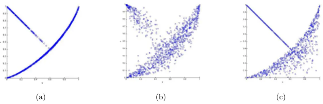
for u, v 2 [0, 1]. The copula of (B1, ˜Bh),⇣Cref,h t ⌘ t 0, is defined by Ctref,h(u, v) = ( v if 1(u) 1(v) p2h t W (u, v) + ⇣ 1(M (u, 1 v)) p2h t ⌘ if 1(u) 1(v) < p2h t
and is admissible for Brownian motions. An illustration is given in Figure3a. One way to construct new copulae from this copula is to consider the dependence between B1and a correlated Brownian
motion to the reflection of B1, see Figure 3b. An other way is to use a random variable for the
barrier, see Figure3cwhere the barrier is equal to h + E with E following an exponential law.
(a) (b) (c)
Figure 3: The Reflection Brownian Copula Cref,h and some of its extensions at time t = 1 with
h = 2. Figure 3a is the Reflection Brownian Copula. Figure 3b is the extension considering a Brownian motion correlated to the reflection of the first Brownian with a correlation ⇢ = 0.95. Figure3cis the extension in the case of a random barrier equals to the sum of h and an exponential random variable with parameter = 2.
Result 1 The copula Cref,h and its extensions are admissible copulae for Brownian motions and
are asymmetric.
Before answering Question 2, let us look to the range of values achievable for P (X Y x) when X and Y are two standard normal random variables, corresponding to the static case of our problem.
Result 2 The range of values achievable for P (X Y x) is ⇥0, 2x ⇤ if we restrict the set of copulae to Gaussian copulae and to⇥0, 2 x
2
⇤otherwise. The supremum bound 2 x
2 is achieved by the copula
Cr(u, v) = (
M (u 1 + r, v) if (u, v) 2 [1 r, 1] ⇥ [0, r],
W (u, v) if (u, v) 2 [0, 1]2\ ([1 r, 1]⇥ [0, r]) with r = 2 ⌘
2 , see Figure 4afor illustration. The copula presents two states of dependence:
the first one corresponds to the countermonotonic copula W , equivalent to a correlation of 1, in the upper left part of the unit square and the second one corresponds to the comonotonic copula M, equivalent to a correlation of 1. The result follows from [47, Section 6.1] and [29;
52; 41] where finding achievable bounds on P (X + Y > x) is considered. The range of values between⇥ x
2 , 2 x 2
⇤
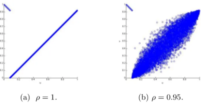
is achieved by considering the copula with a relaxed correlation in the countermonotonic part, see Figure 4.
(a) ⇢ = 1. (b) ⇢ = 0.95.
Figure 4: Patchwork copula Cr(u, v)presenting two states depending on the value of u: the first
copula is in the upper left part of the plan and is W ; the second one is the Gaussian copula with correlation equal to ⇢, with ⇢ = 1 that is the degenerated copula M or ⇢ = 0.95. r is equal to 2 2⌘ with ⌘ = 0.2.
Result 3 is the same than Result 2 but in a dynamical framework and gives an answer to Question 2.
Result 3 The range of values achievable for P B1
t B2t x is h 0, ⇣2px t ⌘i if we restrict the set of copulae to correlation dependence and toh0, 2 ⇣ x
2pt
⌘i
if we consider all admissible copulae for Brownian motions. These values can be achieved using the Reflection Brownian Copula.
The range of values that can be achieved is the same than in the static framework with random variables. An interesting result is that the Reflection Brownian Copula that achieves these values has also two states of correlation: one with correlation equal to 1 and one with correlation equal to -1, as for the copula achieving the upper bound in the static case.
Application to energy commodity prices modeling Spread options are common on energy commodity markets. Let us recall the problem of the producer owning a coal plant with incomes modeled by (St HCt K)+. S and C are modeled by diffusions driven by Brownian motions
and dependence between those Brownian motions is usually modeled by a correlation, implying symmetry in the distribution of St HCt. Nevertheless, coal is a fuel for electricity and HCt is
more likely to be lower than St, which can not be done with a correlation. As marginal models
are satisfying, we only want to change the structure dependence between electricity prices and coal prices, corresponding to the copulae between Brownian motions. Results of this part has shown that to capture asymmetry and higher value for the survival function of the difference of two Brownian motions, one has to consider two states of correlation, one negative and one positive, instead of one. This leads to the two following models:
• A multi-barrier model based on the copula of a Brownian motion and its reflection: we define two barriers ⌫ and ⌘ with ⌫ < ⌘ and we consider two independent Brownian motions X and BY. We construct the Brownian motion Yn that is correlated to ˜Xn: Yn = ⇢ ˜Xn+
p
1 ⇢2BY, with ˜Xn the Brownian motion equal to X at the beginning and reflecting
when X Ynhits a two-state barrier equal to ⌘ before the first reflection and switching from
⌘ to ⌫ or from ⌫ to ⌘ at each reflection.
• A local correlation model with two states of correlation: the local correlation function is chosen such that it is Lipschitz and equal to ⇢1 < 0 when x y ⌫ and to ⇢2 > 0 when
x y ⌘ with ⌘ > ⌫.
These two models seem to be equivalent. Concerning the first model, we derive a closed formula for the cumulative distribution function of the difference between the two Brownian motions. While the second one is more easy to use and understand than the first one, it does not give a closed formula for the cumulative distribution function. Higher values than 1
2 are achieved for P B 1
t Bt2 x
where x 0in both model.
Each commodity price is modeled by a two factor diffusion dfi(t, T ) = fi(t, T )⇣ ise ↵ i(T t) dWts,i+ lidW l,i t ⌘ , i ={Electricity, Coal}.
The parameters are estimated on forward markets of electricity and of coal during 2014 in France with daily observations using the method of [28]. We consider the benchmark model corresponding to dependence modeled by a correlation matrix between the four Brownian motions and the multi-barrier model where the dependence between the two long term Brownian factors are modeled using the multi-barrier model. Modeling the two short term factors using the multi-barrier model has no impact because short term volatilities are too different. Figure5corresponds to the survival function of the difference between products Spot, 1MAH, 3MAH and 6MAH of each commodity for the two models of dependence. Survival function in the multi-barrier model takes higher values than in the benchmark model for x 0 for long term products, which is consistent with the fact that the dependence is changed between the long term Brownian motions. Results are the same considering the local correlation model.
(a) Multi-barrier model. (b) Benchmark model.
Figure 5: Empirical survival function of the difference between the price of electricity and the price of coal at time t = 365 days estimated with 10000 simulations with a time step of 1
24 days for
different products (Spot, 1MAH, 3MAH, 6MAH) in the multi-barrier model and in the benchmark model.
One of the main issue of this model is calibration and the choice of the values of the barrier, that must depends on the initial value of fElectricity(0, T ) HfCoal(0, T )if we want to have more impact
on the survival function of fElectricity(t, T ) HfCoal(t, T ).
3 Second part: Inference of a spike process in high frequency
statistics
A spike is defined as a jump, positive or negative, coming back to 0 in a short period of time. A natural stochastic model for it is a mean reverting jump process with strong mean reversion, see Figure 6. Now, let us consider a stochastic process X defined on a filtered probability space ⇣ ⌦,F, (Ft)0tT,P ⌘ of the form Xt= Z t 0 µsds + Z t 0 sdWs+ Zt, t 0 with Zt = Z t 0 Z Rxe (t s)p (dt, dx) ,
W a standard Brownian motion, µ and two adapted cádlág processes and p a Poisson measure on R+
⇥R independent from W with compensator q = dt⌦⌫ (dx). X is then the sum of a continuous Itô semimartingale and a mean reverting jump process corresponding to the spike process. X is observed on a regular grid M = {ti = i n, 0 i b Tnc} with n = Tn. We assume
that n ! 0 with T fixed, corresponding to a high frequency framework with fixed time horizon.
Our objective is to estimate the parameters of the spike process Z and especially the parameter corresponding to the speed of the mean reversion. If we do not add any further assumptions,
Figure 6: Illustration of a spike process.
the parameter is a drift parameter and is not identifiable if T is fixed ; one can refer to Aït-Sahalia and Jacod [6] for the non identifiability of the drift. Nevertheless, the case in which we are interested is when the mean reversion is strong, corresponding to a spike mode. An illustration is given in Figure 7a: if is too low compared to n, we do not observe the spike effect and
the process does not even revert to 0 before T . To model this spike effect, we need to add the assumption = n ! 1. One has to work under assumption n n . 1 in order to observe all
the spikes: in the other case, a spike can happen and revert to 0 in a period of n and it is not
possible to observe it, see Figure 7b. An non divergence assumption is also needed in the case = n, which is nn . 1: in the other case, the average number of jumps n is stronger than the
speed of mean reversion nand the process diverges as illustrated in Figure7c. An other condition
which is classical is 2
n n ! 0, meaning that there is at most one jump in an interval of size n.
In this framework, there are no results about the identifiability or non identifiability of , raising the following questions.
(a) Low mean reverting. (b) Frequency too high. (c) Number of jumps too high. Figure 7: Spikes processes in non considered regimes.
Question 1 How to identify the jump times and sizes of the spike process in this new framework ?
Question 2 How to estimate the parameter n if it is possible and what is the error of estimation
?
which has been studied by many authors in the literature. One of the main applications is the estimation of volatility in presence of a jump component. The reader can refer to the works of Mancini [42;43], Aït and Jacod [5; 6] or Lee and Mykland [38]. In all these works, the main idea consists in looking to the size of the increments n
iX = Xti Xti 1. This increment can be written
as the sum of the drift increment, the Brownian one and the jump one. As the drift is absolutely continuous with respect to the Lebesgue measure, its increment is of order n. The Brownian
increment is of order p n. The jump increment is of size 1 when there is a jump between times
ti 1and ti and is equal to 0 when there is no jump in this interval. Thus considering a threshold
vn⇣ n$ with $ 2 0,12 , the quantity | n
iX|
p
nvn converges to 0 in the absence of jumps but to 1
in the presence of it.
In our case, the problem is slightly different because there is an extra term caused by the mean reversion after a jump of order n n. In the case n n! 0, it is still possible to distinguish the
jump increment from the mean reversion increment, see Figure8. In the case where n n ⇣ 1, it
is not possible to distinguish a mean reversion increment from a jump increment as they have the same size, see Figure 9. However, we can see that after a jump, the next increment which is the mean reversion one has an opposite sign. One can also show that, under suitable conditions, after a mean reversion increment which is over the threshold vnp n, if there are not too many jumps,
the next increment is of the same sign than the mean reversion one. The following strategy is then adopted: let In(1) < ... <In
⇣
ˆn⌘the indices i 2 {1, ..., n 1} such that • | n
iX| > vnp n if n n! 0,
• | n
iX| > vnp n, inX ni+1X < 0if n n⇣ 1.
We have the following result:
Result 1 With probability converging to 1, ˆn = N1 and Tq 2 ((In(q) 1) n, In(q) n] with
Tq the jump times.
(a) X. (b) niX 0.49 n .
Figure 8: Jump detection in the case n n = 0.3.
Once the spike times are identified, a natural estimator of their size is n
In(q)X for q 2 {1, .., ˆn}
which is equal to XTqe
n(Tq In(q) n) plus an error term with X
Tq the size of the q
(a) X. (b) niX 0.49 n .
Figure 9: Jump detection in the case n n= 1.
The term e n(Tq In(q) n)includes a bias caused by the fact that the jump happens between times
(In(q) 1) nand In(q) nand has already started to mean revert at the moment of observation.
If n n! 0, this term is equal to 1 + O ( n n)and it is possible to identify the size of the jump.
If n n⇣ 1, it is not possible to identify the jump size because we do not know exactly the jump
time. However, if n! 1, it is possible to average this error and we have the following result:
m n n (1 e m n n) ˆn ˆn X q=1 ⇣ n In(q)X ⌘m ! Z Rx m⌫ (dx)
for every integer m > 0 such that RRxm⌫ (dx) <
1. This estimator differs from the classical estimator 1 ˆn Pˆn q=1 ⇣ n In(q)X ⌘m by the term m n n
(1 e m n n): this correction corresponds to the
average error of the bias caused by the mean reversion. To estimate the moments of the jump sizes, one needs to have a consistent estimator of n.
To estimate the parameter n, we consider the slope of the process after a jump
sgn⇣ nIn(q)
⌘
n In(q)+1X
which is of order 1 e n n | X
Tq| where sgn is the sign function. Averaging these quantities
over all the jumps allows to average the noise caused by the Brownian motion. Dividing by an approximation of Pˆn
q=1| XTq|, and taking a logarithm transformation of the average, we obtain
the following estimator bn= 1 n log 0 @ 0 @1 + Pˆn q=1sgn( nIn(q)X) ⇣ n In(q)+1X + 2 n Pq 1 j=1 nIn(j)X ⌘ Pˆn q=1| nIn(q)X| 1ˆn>0 1 A _ n 1 A .
where a correction term 2 nPq 1j=1 nIn(j)X is added in order to avoid a bias term of order n n.
Result 2 The error bn n
n is equal to Op ⇣ n n+ min ⇣ n n, 1 2 n ⌘ + np n n 1⌘ and a cen-tral limit theorem is given under some asymptotic assumptions.
The first error term is a bias term, the second one is due to noise caused by previous jumps that have not revert to 0 entirely and the third one is caused by the Brownian motion. In order for the estimator to be consistent, we need to have the Brownian motion error np n n
1
! 0 as the two first errors terms converge to 0. This condition can be explained by the fact that the size of the noise due to an increment of the Brownian motion is of orderp n, the one due to the average
of increments happening after a jump is then of orderq n
n and the size of the mean reversion if
of order n n. For the noise to be negligible compared to the estimator which is the slope, it is
needed to haveq n
n = o ( n n), corresponding to our condition.
Application to spike modeling in electricity time series Let us generalize the two factor model in order to have a spike component. We model the forward price f (t, T ) under the historical probability by f (t, T ) = Z t 0 µsds + fc(t, T ) + Z t 0 Z Rxe (T s)p (ds, dx) where dfc(t, T ) = fc(t, T )⇣ se ↵(T t)dWs+ ldWl ⌘
corresponds to the classical forward dynamics. The spot price is then equal to St= Z t 0 µsds + Stc+ Z t 0 Z Rxe (t s)p (ds, dx)
where Sc is the equivalent spot model of the two factor model and is a semimartingale. We have
established a simple model on the forward and the spot, that differs only slightly from the classical models by adding a spike component. We apply our estimation procedure on French, German and Australian spot prices to estimate the spike component. When we compute the forward products f (t, T, ✓), the component due to f is of order which is negligible compared to the continuous part of the forward. The spot factor has not impact on the forward prices, which is consistent with the data. The parameters of the continuous part of the model can then be estimated on the forward products as there were no spikes. The continuous part is calibrated on the French forward products. Figure 10corresponds to one simulation of the models with and without spikes using estimated parameters on French market and shows that the spike factor has no impact on forward products prices but only on the spot. We also show that spike modeling has also a strong impact on strips of call options pricing of the form RT
0 (St K) +dt.
4 Third part: Non parametric estimation of the intensity of
a doubly stochastic Poisson process depending on a
covari-able
In this part, we are interested in a continuous semimartingale X and in a doubly stochastic Poisson process N defined on the common filtered probability space⇣⌦,F, (Ft)0tT,P
⌘
. The law of the doubly stochastic Poisson process is entirely determined by its intensity function which is also a stochastic process. Modeling the dependence between N and X is then the same as modeling
(a) Spot. (b) 1WAH.
(c) 1MAH.
Figure 10: Simulation of different products in a two factor model with and without spikes between the 27th of February 2017 and the 31st of March 2017. We illustrate the spot, the 1WAH starting
the 27th of February 2017 and the 1MAH starting the 01st of March 2017.
the dependence between and X. We assume that X and N are observed continuously on a time horizon [0, T ]. We assume that
s= nq (Xs) , s2 [0, T ]
where n 2 N, n 1 corresponds to the asymptotic. Conditionally on (Xt)0tT, N is an
inhomo-geneous Poisson process with intensity at time t nq (Xt). Our objective is to estimate the function
qon a given interval I of R. The literature on non parametric estimation of intensity function for Poisson processes is large. The simplest case corresponds to the inhomogeneous Poisson process where the intensity is a deterministic function of the time: [50;51] use model selection techniques and projection estimators in a non asymptotic framework. A penalization function is proposed in oder to select the optimal model. [26; 15] use kernel estimators in an asymptotic framework ; in [15], a method to select the bandwidth is proposed. Most used doubly stochastic Poisson process models are the one of Aalen and Cox [1; 23]. In the Aalen model, the intensity function is of the form ↵tYt with ↵t a function of time and Yt a stochastic process. In the Cox model, it is of
the form ↵texp TZ with Z a multi-dimensional random variable or stochastic process in some
cases (see [45] for instance). Again, projection estimators are used by [22] and local polynomial estimators which are generalization of kernel estimators are used by [21] for those models. In [60], the intensity of a doubly stochastic Poisson process is inferred as a function of time using kernel methods in an asymptotic framework. To our knowledge, non parametric methods of estimation in our framework is less common in the literature except for [56] that proposes a kernel estimator of the function q in the case where T goes to 1 and when X satisfies some conditions, which can be for instance stationarity. We want to work in a more general framework when X does not need
to be stationary.
First, in order to estimate the function q at some point x 2 I, we need for X to be close to x a certain amount of time before T . One way to evaluate the time spend by X around x when X is a semimartingale is the local time lx
T. We consider the natural local time of X being the measure
verifying the occupation time formula Z t 0 f (Xs) ds = Z Rf (x) l x tdx, 0 t T
for any measurable function f on ⌦⇥R. It differs from the classical local time used in the literature where the integration of the left hand side is with respect to dhXis [49, Chapter 6] but both are
linked. lx
T can also be defined by
lim ✏!0 1 2✏ Z T 0 1|Xs x|✏ds.
If we write Xt=R0tµsds +R0t sdWs, a sufficient condition for the existence of lxT is inf s2[0,T ] s
almost surely with > 0 a constant. Adding the assumption E✓RT
0 |µs|ds + sup 0tT | RT 0 sdWs| ◆ < 1, we have E ✓ sup x2R lx T ◆
<1 which is needed in this part. All these results can be derived easily using [49, Exercise 1.15] and [7, Equation (III) ]. We also consider the degenerated case Xt = t
corresponding to the inhomogeneous Poisson process. We then work under one of the following assumptions:
(i) inf
0sT s with > 0 a deterministic constant and
E Z T 0 |µ s|ds + sup 0tT| Z T 0 sdWs| ! <1,
(ii) Xt= t for all t in [0, T ].
In order to estimate q at point x 2 I, we then need to have lx
T > 0. We then choose to work
conditionally on the event D (I, ⌫) defined by D (I, ⌫) ={! 2 ⌦, inf x2Il x T(!) ⌫T |I|}
with ⌫ 2 (0, 1]. This framework is the same as the one of [33] in the context of non parametric estimation of the volatility function (Y ) of a diffusion Y .
Let K be a positive kernel function with bounded support [ 1, 1], kKk1 = sup x2R
K (x) < 1, Kh(x) = h 1K xh for x 2 R and h > 0 the bandwidth parameter. We consider the local
polynomial estimator of q with degree m for h > 0 and x 2 R ˆ qh(x) = 1 n Z T 0 w ✓ x, h,Xs x h ◆ Kh(Xs x) 1Xs2IdNs
with U (x) = ✓ 1, x,x 2 2!, .., xm m! ◆T , w (x, h, z) = UT(0) B (x, h) 1U (z) 1B(x,h)2S+ m+1, z2 R and B (x, h) = Z T 0 U ✓ Xs x h ◆ UT ✓ Xs x h ◆ Kh(Xs x) 1Xs2Ids. If B (x, h) 2 S+
m+1, this estimator is equal to UT(0) ˆ✓h(x)with
ˆ ✓h(x) = argmin ✓2Rm+1 2 n✓ TZ T 0 U ✓ Xs x h ◆ Kh(Xs x) 1Xs2IdNs + ✓T Z T 0 U ✓X s x h ◆ UT ✓X s x h ◆ Kh(Xs x) 1Xs2Ids✓.
We denote by qhthe conditional expectation of ˆqh given X:
qh(x) = Z T 0 w ✓ x, h,Xs x h ◆ Kh(Xs x) 1Xs2Iq (Xs) ds.
On the event D (I, ⌫), if there exists > 0and Kmin> 0such that K (x) Kmin1|x| for x 2 R,
we prove that B (x, h) 2 S+
m+1 for x 2 I and 0 < h 23 |I|.
In order to evaluate the performance of our estimator, we choose to work with the integrated quadratic loss on I, conditionally on D (I, ⌫), that is with the quantity E kq ˆqhk2I|D (I, ⌫)
where kfk2
I is equal to
R
If (x)
2dx. We want to answer the following questions:
Question 1 How to choose the bandwidth parameter h in an optimal way ? Question 2 What is the speed of convergence of our estimator and is it optimal ? Question 3 Is the function q belongs to some parametric family ?
Question 1 is central because the bandwidth parameter has an impact on the quality of our estima-tor and Question 2 will assess its quality in terms of speed convergence. Question 3 has operational purposes: it is easier in terms of comprehension and modeling to work with a parametric function than a non parametric one.
The loss function can be written as the sum of a bias term E kq qhk2I|D (I, ⌫) decreasing with h
and a variance term E kqh qˆhk2I|D (I, ⌫) increasing with h. The bandwidth h that minimizes the
sum of the bias and the variance is then optimal in the sense that the loss function is minimized. However, this optimal bandwidth depends on q that we do not know and is called the oracle bandwidth. One wants to choose a bandwidth h such that the value of the loss function is close to the oracle one. The same issue exists for density estimation where the observations are i.i.d. random variables, see the discussion in [55, Section 1.8].
One solution is to give unbiased estimators of the bias and the variance terms and to choose for the bandwidth h the one minimizing the sum of the two. While an unbiased estimator of the variance term is easily to find, the main issue is the approximation of the bias term. In the i.i.d case, the variance term is deterministic and known but in our case, an unbiased estimator of it is given by
ˆ Vh= 1 n2 Z T 0 Z I ✓ w ✓ x, h,Xs x h ◆ Kh(Xs x) ◆2 1Xs2IdxdNs.
Concerning the estimator of the bias term, in a context of i.i.d observations with a kernel estimator, [37] proposes to approximate the bias kq qhk2I by kq qhmink
2
I with hmin sufficiently small. If
hmin! 0, the bias kqhmin qk
2
I ⇡ 0 and kqhmin qhk
2
I ⇡ kq qhk2I. This method is derived from the
classical Goldenshluger Lepski method [30;39]. We adapt the method of [37] to the Poisson process framework but also to the local polynomial framework. An unbiased estimator of kqhmin qhk
2 I is given by kˆqhmin qˆhk 2 I Vˆh Vˆhmin+ 2 ˆVh,hmin
with ˆVh,hmin equals to
1 n2 Z T 0 Z I w ✓ x, h,Xs x h ◆ Kh(Xs x) w ✓ x, hmin, Xs x hmin ◆ Khmin(Xs x) 1Xs2IdxdNs.
At the end, we select the following bandwidth ˆ
h = argmin
h2H kˆqhmin qˆhk 2
I Vˆh+ 2 ˆVh,hmin+ ˆVh
among a finite set H included in (0, 1) with > 0 an hyper parameter chosen by the statistician. We assume that min H = hmin kKk1kKkn 1|I|, with kKk1 =RR|K (u) |du and max H 23|I| .
This choice of bandwidth leads to the following result. Result 1 Assume sup
x2I
q (x) <1. The loss E kq qhk2I|D (I, ⌫) is bounded by the sum of
✓ _ 1 + O⇣log (n) 1⌘◆min h2HE ||ˆqh q|| 2 I|D (I, ⌫) and O (log (n))E ||qhmin q|| 2 I|D (I, ⌫) + 1 ⌫2O log (n_ |H|)6 n ! .
Result 1 consists in an oracle inequality that is derived from the two concentration inequalities [51, Equation (2.2)] and [34, Theorem 4.2]. The error term of order log (n) E ||qhmin q||
2
I|D (I, ⌫) is
caused by the approximation of kq qhk2I by kq qhmink
2
I. The error coming from this term depends
of the regularity of q. The term 1
⌫2 corresponds to an error caused by the quantity of observations
of X in I and if it is small, it leads to more error. When n is large, and if = 1, our choice of bandwidth gives values of the loss close to the optimal one if log (n) E ||qhmin q||
2
I|D (I, ⌫) is
enough small.
Result 1 does not give information about the quality of our estimator. For ⇢, , L > 0, let ⇤⇢, ={f : I ! R : f (x) ⇢, sup
x2I f (x) <1} \ ⌃ ( , L, I) where ⌃ ( , L, I) is the Hölder class
of order on I with bounding constant L. Result 2 and Result 3 assess the performance of ˆqhˆ
in the minimax sense over ⇤⇢, and answer to Question 2. We recall that m is the degree of the
estimator polynomial.
Result 2 The sequence E '2
nkq qˆˆhk2I|D (I, ⌫) is bounded uniformly over ⇤⇢, with 'n equals
to n2 +1 if m b c and n m
Result 3 The rate of convergence n2 +1 is a lower bound in the minimax sense.
Then, if m b c, our estimator in optimal in the minimax sense with rate of convergence n2 +1.
To answer Question 3, we propose to test ⇢
H0: 9✓02 ⇥, q = g✓against
H1: 8✓ 2 ⇥, q 6= g✓
with ⇥ ⇢ Rd, d 1 and g
✓ a function parametrized by ✓. Let us consider the contrast
Mn(✓) =kˆqhˆ(·) Z T 0 w ✓ ·, ˆh,Xsˆ · h ◆ Kˆh(Xs ·) 1Xs2Ig✓(Xs) dsk 2 I 1 n2 Z I Z T 0 w2 ✓ x, ˆh,Xsˆ x h ◆ Kˆh2(Xs x) 1Xs2IdNsdx.
The second term is a bias correction term in order to have an asymptotic unbiased estimator. The first term measures the distance between ˆqˆhwhich is an estimator of q under both hypothesis and
g✓, or rather a biased version of it allowing to avoid a bias term in this distance. This contrast
converges in probability to kq g✓k2I and a natural estimator of ˆ✓n of ✓0 under H0 is
ˆ ✓n= inf
✓2⇥Mn(✓) .
A way to test H0is to look at Mn
⇣ ˆ ✓n
⌘
that is small under H0but diverges under H1.
Result 4 Under H0, ˆ✓n converges to ✓0 at the rate n
1
2 and a critical region of the test at level
↵is |Mn ⇣ ˆ ✓n ⌘ | c (↵) = nˆ 1ˆh 12 q ˆ Vn 1 ⇣ 1 ↵ 2 ⌘ where ˆ Vn= C (K) Z I g✓ˆn(y) RT 0 Kˆh(y Xs) 1Xs2Ids !2 dy,
C (K)is a constant depending only of K and is the cumulative distribution function of a N (0, 1) random variable.
A central theorem is also given for ˆ✓n. Result 4 indicates that Mn
⇣ ˆ ✓n
⌘
converges to 0 in probability at the convergence rate n 1ˆh 1
2 under H0 and to 1 under H1. This test is similar to the one of
[4] used to test if the drift and volatility of a diffusion belong to some parametric family.
Application to dependence modeling between electricity spot prices and wind produc-tion Following the ideas of [58], we study the dependence between the electricity spot price and the wind penetration index in Germany. The wind penetration index is defined as the ratio between the wind production and the total electricity production. Data considered are the hourly German spot price and hourly wind penetration index between year 2012 and 2016, both included. Our intuition is that high wind penetration index leads to negative spikes in electricity spot price time
series. Spikes are modeled by a strong mean reverting Poisson process, as in Chapter 3. Method of Chapter 3 is then used in order to detect the spikes in the spot time series. We distinguish positive and negative spikes and estimate the intensity of the point process as a function of the wind penetration index for each process using the local polynomial estimator of Chapter4of order 0, that is with kernel, see Figure 11a and Figure11b. Using the parametrical test, we test if the two intensity functions are constant: the test is not rejected for positive spikes but is for negative ones with a confidence level at 95%. We also find an increasing function of the wind penetration for the negative spikes intensity.
(a) For negative spikes. (b) For positive spikes.
Figure 11: Kernel estimators of the intensity of the spot spikes as a function the wind penetration. Based on these results, the spot price is modeled as the sum of a seasonality function, a continuous autoregressive process and two spikes process: one for the positive spikes and one for the negative ones, both having the same mean reversion. The intensity of the positive spike process is modeled by a constant but the one of the negative one has two states: a low intensity for low wind penetration values and a high intensity for high wind penetration values, see Figure11a. Concerning the wind penetration index, as its values lie between 0 and 1, its logit is modeled by the sum of a seasonality function and a continuous autoregressive process of order 24. Methods of estimation are provided for both models.
In order to study the impact of our modeling, one consider the point of view of an electricity company buying electricity to an wind producer at a fixed price K. The wind producer produces Q% of the total wind production. The incomes of the electricity company over a period T are then equals to QR0TCtW Pt(St K) dt where Ct is the total load. Value at Risk and Expected
Shortfall of this model are compared to the ones of the model where the intensity of negative spikes is constant: the difference is significant between the two models.
5 Structure of the thesis
The thesis is composed of five chapters based on the following works:
- [Chapter 1] On the control of the difference between two Brownian motions: a dynamic copula approach, published in Dependence Modeling.
- [Chapter 2] On the control of the difference between two Brownian motions: an application to energy markets modeling, published in Dependence Modeling.
- [Chapter 3] Estimation of a fast mean reverting jump process with application to spike modeling in electricity prices, joint work with O. Féron and M. Hoffmann.
- [Chapter 4] Local polynomial estimation of the intensity of a doubly stochastic Poisson process. - [Chapter 5] A joint model for electricity and wind penetration with dependence in the electricity spikes, joint work with A. Veraart, submitted in Forecasting and Risk Management for Renewable Energy 2017: Conference proceedings.
[1] Odd Aalen. Nonparametric inference for a family of counting processes. The Annals of Statistics, pages 701–726, 1978.
[2] René Aid, Luciano Campi, Adrien Nguyen Huu, and Nizar Touzi. A structural risk-neutral model of electricity prices. International Journal of Theoretical and Applied Finance, 12(07):925–947, 2009.
[3] René Aid, Luciano Campi, and Nicolas Langrené. A structural risk-neutral model for pricing and hedging power derivatives. Mathematical Finance, 23(3):387–438, 2013.
[4] Yacine Ait-Sahalia. Testing continuous-time models of the spot interest rate. Review of Financial studies, 9(2):385–426, 1996.
[5] Yacine Aït-Sahalia and Jean Jacod. Testing for jumps in a discretely observed process. The Annals of Statistics, pages 184–222, 2009.
[6] Yacine Aït-Sahalia and Jean Jacod. High-frequency financial econometrics. Princeton Uni-versity Press, 2014.
[7] Martin T Barlow and Marc Yor. Semi-martingale inequalities via the garsia-rodemich-rumsey lemma, and applications to local times. Journal of functional Analysis, 49(2):198–229, 1982. [8] Fred Espen Benth. Cointegrated commodity markets and pricing of derivatives in a
non-gaussian framework. In Advanced Modelling in Mathematical Finance, pages 477–496. Springer, 2016.
[9] Fred Espen Benth, Jan Kallsen, and Thilo Meyer-Brandis. A non-gaussian ornstein–uhlenbeck process for electricity spot price modeling and derivatives pricing. Applied Mathematical Finance, 14(2):153–169, 2007.
[10] Fred Espen Benth and Paul C Kettler. Dynamic copula models for the spark spread. Quan-titative Finance, 11(3):407–421, 2011.
[11] Fred Espen Benth and Steen Koekebakker. Stochastic modeling of financial electricity con-tracts. Energy Economics, 30(3):1116–1157, 2008.
[12] Fred Espen Benth, Nina Lange, and Tor Age Myklebust. Pricing and hedging quanto options in energy markets. Journal of Energy Markets, 2015.
[13] Tomasz R Bielecki, Jacek Jakubowski, Andrea Vidozzi, and Luca Vidozzi. Study of depen-dence for some stochastic processes. Stochastic analysis and applications, 26(4):903–924, 2008.