Analyse de vitesse par migration quantitative dans les domaines images et données pour l’imagerie sismique

(1)

HAL Id: tel-01814262

https://pastel.archives-ouvertes.fr/tel-01814262

Submitted on 13 Jun 2018

HAL is a multi-disciplinary open access archive for the deposit and dissemination of sci-entific research documents, whether they are pub-lished or not. The documents may come from teaching and research institutions in France or abroad, or from public or private research centers.

L’archive ouverte pluridisciplinaire HAL, est destinée au dépôt et à la diffusion de documents scientifiques de niveau recherche, publiés ou non, émanant des établissements d’enseignement et de recherche français ou étrangers, des laboratoires publics ou privés.

domaines images et données pour l’imagerie sismique

Yubing Li

To cite this version:

Yubing Li. Analyse de vitesse par migration quantitative dans les domaines images et données pour l’imagerie sismique. Géophysique [physics.geo-ph]. Université Paris sciences et lettres, 2018. Français. �NNT : 2018PSLEM002�. �tel-01814262�

(2)

THÈSE DE DOCTORAT

de l’Université de recherche Paris Sciences et Lettres

PSL Research University

Préparée à MINES ParisTech

Subsurface seismic imaging based on inversion velocity

analysis in both image and data domains

Analyse de vitesse par migration quantitative dans les

domaines images et données pour l’imagerie sismique

École doctorale n

o

398

GÉOSCIENCES, RESSOURCES NATURELLES ET ENVIRONNEMENT

Spécialité

GÉOSCIENCES ET GÉOINGÉNIERIE

Soutenue par

Yubing LI

le 16 janvier 2018

Dirigée par

Hervé CHAURIS

COMPOSITION DU JURY :

M Jean-Pierre VILOTTE Président IPGP

M Gilles LAMBARÉ Rapporteur CGG

M William SYMES Rapporteur Rice University

M Romain BROSSIER Membre du jury Université Grenoble Alpes

Mme Céline GÉLIS Membre du jury IRSN

M Hervé CHAURIS Membre du jury MINES ParisTech

M François AUDEBERT Membre du jury Total

(3)

(4)

Acknowledgments

I would like to thank all the people who have contributed to this thesis work. There is a saying: "If you want long memory, you need a short pencil." I hope that I could always remember all the great memories for this period of my life.

I would like to express my sincere gratitude to my advisor, Professor Hervé Chauris, for offering me the opportunities to do an internship and to pursue the PhD at MINES ParisTech. I thank him for his patience, support and encouragement. Hervé even would like to help me with the very details of the code and with the basic formulations. He always provided useful instructions and inspirations when I was obstructed by difficul-ties. He has a healthy attitude towards life and I can always feel his kind heart to me. I am very grateful to him for helping me organize the defense and revise the manuscript line-by-line. His passion for the research encourages me a lot.

I would like to thank the members of my jury. It was my great honor that William Symes and Gilles Lambaré accepted to review my thesis in detail. I thank them for the professional comments and the fruitful recommendations. My sincere thanks also goes to Jean-Pierre Vilotte for chairing the defense and to Romain Brossier, Céline Gélis and François Audbert for examining my work.

I thank Paris Exploration Geophysics Group (GPX) for financially supporting my thesis. All the research described in this thesis was carried out as a part of the GPX project funded by the French National Research Agency, CGG, Total and Schlumberger. I thank the GPX committee, especially Satish Singh, Hervé Chaursi and Mark Noble, for accepting my Master application four years ago. It offered me the chance to come to France and to subsequently pursue my PhD. I thank Nobuaki Fuji for kindly helping me to get access to the S-CAPAD platform at IPGP for more computational resources.

Many thanks to the members of the geophysics team at MINES ParisTech. I espe-cially thank Véronique Lachasse for her help to facilitate the administrative affairs since my day one in Fontainebleau. I sincerely thank the permanent researchers, Daniela Donno, Pierre Dublanchet, Alexandrine Gesret and Mark Noble, and the scientific vis-itors, Nidhal Belayouni and Pierre-François Roux, for their kindness. I also would like to thank all my colleagues during the three and half years, Elise Vi Nu Bas, Charles-Antoine Lameloise, Emmanuel Cocher, Sven Schilke, Yves-Marie Batany, Tiago Bar-ros, Jihane Belhadj, Julien Cotton, Hao Jiang, Keurfon Luu, Alexandre Kazantsev,

(5)

Michelle Almakari, Tianyou Zhou, Ahmed Jabrane Maxime Godano, Shanker Krishna, Zufri and Joshua Lartey., for their friendship and support. I express my special thanks to Emmanuel for guiding me to the CROUS residence on the first day and to Hao for selecting the defense gift as the representative of others on the last day. First day, last day, everyday was a nice day.

In addition, I want to thank my lovely friends who have supported me in France. Some of them were also doing research, giving me broader views and different ideas in science. Some of them had different paths of life but we did get along with each other. I give my acknowledgement to Quan Chen, Wei Li, Shuqiao Zou, Fuchen Liu, Shizhu Zheng, Dandan Niu, Shihao Yuan, Yanfang Qin, Weiguang He, Haiyang Wang, Xin Gao, Hanchao Jian, Jialan Wang, Zhengbin Deng, Dongyang Huang, Miao Yu, Han-jun Yin, Shaozhuo Liu, Xiangdong Song, Zezhong Zhang, Shuaitao Wang, Tianyuan Wang, Shun Huang, Mingguan Yang, Feng Yang, Botao Qin, Kurama Ohkubo, Eke-abino Momoh, Pierre Romanet, Mohammad Shahrukh, Fernando Villanueva-Robles, Alvina Kusumadewi and others.

I would express a deep sense of gratitude to my beloved family for their consistent support and unconditional love. My research would not have been possible without the contribution of my dearest parents, who have given me life and have always stood by me like a pillar in times of need. Special thanks are due to my one and only loving sister Ruiyun Li who stays close to our parents and keeps them feel less lonely.

Finally, I want to acknowledge my sweet wife Yanhui He who has been accompa-nying me during these important but happy years. It is my fortune to meet you, to love you and to have you by my side for the rest of my lifetime. Life is a long journey: you were and always will be the most impressive part of my grand tour, mon amour.

(6)

Abstract

Active seismic experiments are widely used to characterize the structure of the subsur-face for the oil and gas industry. Based on the assumption of scale separation, numer-ous approaches split the velocity model into a smooth background model controlling the kinematics of wave propagation and a reflectivity model characterizing the rapid changes of the model parameters. Macro velocity estimation and reflectivity imaging are formulated as two inverse problems. The macro velocity estimation scheme can be derived either in the data-domain, where one seeks an optimal fit between modeled and observed data, or in the image-domain, where one tries to improve the image coherency. Migration techniques aim at determining the reflectivity in a given macromodel. Classic migration is the adjoint operator of the forward linearized modeling and suffers from migration artifacts. Recent studies recast the asymptotic inversion in the context of reverse time migration. They define a direct way for inverting the Born modeling operator, which automatically compensates for uneven illuminations and geometrical spreading losses, removing in practice migration artifacts.

Migration Velocity Analysis (MVA) techniques assess the quality of the estimated macromodel by observing the migrated images. The analysis is carried out on the panels called common image gathers. These panels can be built in two manners: the surface-oriented methods first perform prestack migration on different subsets of input data, such as the common-shot gathers, and then collect images along the redundant parame-ter; the depth-oriented methods extend the image volume with an additional parameter, for example the subsurface-offset as a spatial delay, inserted during the construction of reflectivity images. Recent investigations propose to couple the direct inversion to MVA in the subsurface-offset domain, introducing better robustness. This approach is numer-ically demanding, even in 2D, and cannot be currently extended to 3D. In this thesis, I propose to transpose this strategy to the more conventional common-shot migration based MVA.

I first develop an alternative approach to a recent published work, related to the common-shot true-amplitude reverse time migration. It is a pseudo-inverse of the Born modeling operator in the asymptotic sense. The method allows producing prestack re-flectivity images free of migration smiles in a direct way. Then, I propose to couple this operator to velocity analysis. Inversion Velocity Analysis (IVA) is thus an alternative

(7)

to MVA consisting of replacing migration by an asymptotic inverse. I analyze how the approach can deal with complex models, in particular with the presence of low velocity anomaly zones or discontinuities, better than the classic MVA. Common-shot IVA ben-efits from the natural parallel implementation, and requires less numerical cost than its counterpart in the subsurface-offset domain.

I also propose to extend IVA to the data-domain, leading to a more linearized inverse problem than classic full waveform inversion. It simply consists of applying the model-ing operator to the images after the application of the annihilator. The new approach is close to Full Waveform Inversion, in the sense that the optimal model is obtained when the norm of the data residual is minimum. On the other hand, the new approach is still based on the coherency criteria for which the inverse problem is known to have a better convexity, at least for simple models. I compare the new approach to other reflection-based waveform inversion to establish formal links between data-fitting principle and image coherency criteria.

The methodologies are analyzed on 2D synthetic data sets from a series of veloc-ity models, in particular models with the presence of a low-anomaly zone for which common-shot migration is not necessarily appropriate, and the Marmousi model, to justify the robustness. The main contribution of this work is (1) the development of common-shot true-amplitude reverse time migration and, more importantly, the cou-pling with velocity analysis; (2) the extension of common-shot IVA to the data-domain and, along this line, the analysis of the links between image-domain and data-domain methods.

(8)

Résumé

Dans le domaine de la prospection pétrolière, les expériences sismiques actives sont lar-gement utilisées pour caractériser la structure de la subsurface. Avec l’hypothèse de la séparation des échelles, de nombreuses approches divisent le modèle de vitesse entre un modèle de grande longueur d’onde qui contrôle la cinématique de propagation des ondes, et un modèle de réflectivité qui caractérise les changements rapides. Les esti-mations du macro-modèle de vitesse et de la réflectivité sont formulées comme deux problèmes inverses imbriqués. La détermination du macro-modèle peut être obtenue soit dans le domaine des données, où est mesurée l’écart entre les données modélisées et les données observées, ou dans le domaine image, où l’objectif est d’avoir des images cohérentes.

Les techniques de migration visent à déterminer le modèle de réflectivité dans un macro-modèle donné. La migration classique est seulement l’adjoint de l’opérateur de modélisation linéarisé. La méthode est connue pour causer des artefacts de migration. Récemment, une formule d’inversion au sens asymptotique a été développée pour rem-placer la migration. C’est une méthode directe sans itération. Elle compense pour l’illu-mination irrégulière, pour le facteur d’atténuation géométrique et donne des images beaucoup plus propres en pratique.

L’analyse de vitesse par migration est une technique qui juge de la qualité d’un macro-modèle de vitesse en comparant différentes images issues de sous-ensembles des données, comme par exemple un point de tir. Des panneaux sont construits en modifiant la condition d’imagerie soit avec un paramètre de surface, soit avec un paramètre lié à la profondeur, comme un délai en espace ou en temps. Des résultats récents proposent de coupler l’inversion asymptotique avec l’analyse de vitesse pour la version extension en profondeur. L’analyse de vitesse est rendue beaucoup plus robuste. Cette approche cependant demande des capacités de calcul et de mémoire importantes, même en 2D, et ne peut actuellement être étendue en 3D. Dans ce travail, je propose de développer le couplage entre l’analyse de vitesse et la migration plus conventionnelle par point de tir. Je développe dans un premier temps une alternative à un travail récent autour de la migration quantitative par point de tir. La formule est un pseudo-inverse de l’opéra-teur de Born au sens asymptotique. Elle permet d’obtenir des images migrées propres sans recourir à des itérations. Ensuite, je propose de coupler cet opérateur inverse avec

(9)

l’analyse de vitesse dite par inversion et non plus par migration. La nouvelle approche permet de prendre en compte des modèles de vitesse complexes, comme par exemple en présence d’anomalies de vitesses plus lentes ou de réflectivités discontinues. C’est une alternative avantageuse en termes d’implémentation et de coût numérique par rapport à la version profondeur.

Je propose aussi d’étendre l’analyse de vitesse par inversion au domaine des don-nées. Ceci conduit à une approche du problème inverse plus linéarisée que celle de l’in-version des formes d’onde. Il suffit d’appliquer l’opérateur de modélisation aux images après la multiplication par l’annihilateur. Cette nouvelle approche est proche de l’inver-sion des formes d’onde dans le sens que le modèle optimal est obtenu lorsque la norme des résidus est minimale. D’un autre côté, l’approche est toujours basée sur le critère de cohérence. Le problème inverse est connu pour être plus convexe, au moins pour des modèles simples. Je compare la nouvelle approche avec d’autres méthodes pour établir des liens formels entre des méthodes dans le domaine des données et dans le domaine des images.

Les méthodologies sont analysées sur les jeux de données 2D et au travers de toute une série de méthodes de vitesse, en particulier des modèles avec la présence de zones de vitesses plus faibles à l’origine de triplications. Ces modèles ne sont pas nécessairement appropriés pour la migration par point de tir. J’applique aussi les méthodes au modèle Marmousi pour tester la robustesse. Les principales contributions de ce travail sont (1) le développement de la migration par point de tir avec amplitude préservée, et surtout le couplage avec l’analyse de vitesse ; et (2) l’extension de l’analyse de vitesse au domaine des données, et le lien entre les domaines données et images.

(10)

List of Figures

1.1 Acquisition geometries for land and marine environments. . . 5 1.2 A synthetic example of marine seismic data acquired at the surface: (a)

scattered paths in the model; (b) transmitted paths in the model; (c) shot gather recorded at the surface. The red star denotes the position of the source. Solid, dot dashed and dashed white lines in (a) denote first-reflected, multi-reflected and multi-diffracted waves, respectively. Solid, dot dashed and dashed white lines in (b) denote direct, diving and refracted waves, respectively. . . 7 1.3 In black, the classic sketch byClaerbout (1985) illustrating the spatial

frequencies that can be resolved from seismic data. The gap is now filled by the improved resolution of tomography (red curve) and by the impact of broadband acquisition on imaging (blue curve) (fromLambaré et al.,

2014). . . 8 1.4 A synthetic example of the scale separation for the Marmousi model.

The full velocity model (left) is decomposed into a smooth background velocity model (middle) and a velocity perturbation model (right). . . . 8 1.5 Schematic for local optimization methods. . . 11 1.6 Illustration of the relationship between the wavenumber k = ks+ krand

the opening angle θ (adapted fromAlkhalifah and Plessix,2014). . . 14 1.7 Illustration of the origin of cycle skipping effect. Local optimization

converges towards the global minimum for the modeled data with smaller time shift error (left pink circle), whereas it converges towards the local minimum for the modeled wavelet with larger time shift error (red star). The black arrows mark the descent directions. . . 15 1.8 Same as for Figure 1.7, but the low-frequency content is involved in

the observed and modeled data. The cycle skipped case (red star) in Figure 1.7 now converges towards the global minimum with the help of low-frequency. . . 16 1.9 The principle of Born modeling: (a) calculation of traveltime; (b)

Kirch-hoff hyperbola on seismogram. (adapted fromPyun and Shin,2008) . . 17 1.10 Description of imaging condition for a simple reflector. . . 18 1.11 Description of iterative migration. . . 19

(15)

1.12 Illustration indicating that migration cannot completely reproduce the data: (a) observed data, (b) migrated image with correct macro velocity model, and (c) modeled data with image (b) in the correct macro velocity model. The artificial direct arrivals in panel (c) correspond to migration artifacts in panel (b). The observed and modeled data are in phase, but their amplitudes are different. . . 19 1.13 Conventional RTM (a) and least-squares RTM (b) images of the

syn-thetic salt model based on a GOM survey (adapted from Zeng et al.,

2017). . . 21 1.14 Prestack common-offset data before (a) and after (b) migration. Seismic

data set computed in 2D Marmousi model (a), migrated to surface-offset domain CIGs (b) by prestack depth migration using the true velocity model. A and C are common-offset gather and prestack migrated image, respectively, at zero-offset. B and D are common midpoint gather and CIG, respectively, at fixed position. Accurate velocity model results in flatness on the CIG panel D. (fromChauris,2000) . . . 27 1.15 Examples illustrating the impact of migration artifacts on image

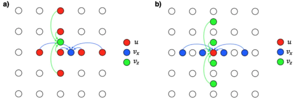
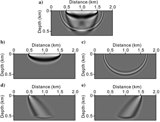
differ-ences, for a single reflector embedded in a homogeneous macro velocity model. (a) corresponds to the exact reflectivity model, (b) to the image migrated in the correct macro velocity model for a single shot marked by green point in (a), and (c) to the difference between image (b) and the image for an adjacent shot. (d–e) are similar to (b–c), but for an incorrect model of which the velocity is 5% lower than the correct value. Black ellipses correspond to the upward-curved events attributed to velocity inaccuracies, and green ellipse to those attributed to migration smiles. . 31 1.16 Same as for Figure 1.15, but for the Marmousi model. . . 32 2.1 Description of the grid points needed to update (vx, vx) (a) and u (b)

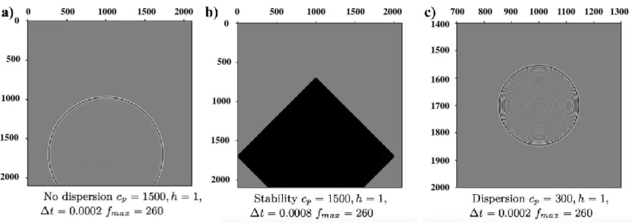
fields (adapted fromThorbecke,2015). For both cases, four neighbour-ing points are needed to compute one central point. . . 41 2.2 Snapshots of wavefields for the case of stable result (a), of instability

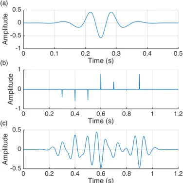
(b), and of dispersion (c) (adapted fromThorbecke,2015). . . 42 2.3 The construction of synthetic data: (a) the source wavelet, (b) the

ran-dom pulses and (c) the convolution between the wavelet and ranran-dom pulses. . . 46

(16)

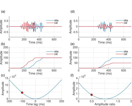
List of Figures xiii 2.4 Investigation of the shape of the `2 norm OF: (a) observed data (blue)

and calculated data with shifted phase (red); (b) misfit curve related to different phase shifts (blue curve) and the misfit corresponding to calcu-lated data in (a) (red dot); (c) observed data (blue) and calcucalcu-lated data with varying amplitude terms (red); (d) misfit curve associated to differ-ent amplitude ratios (blue curve) and the misfit corresponding to calcu-lated data in (a) (red dot). . . 47 2.5 Same as Figure 2.4, but for the normalized crosscorrelation OF. . . 49 2.6 Same as Figure 2.4, but for the AWI OF. . . 50 2.7 Same as Figure 2.4, but for the logarithmic envelop OF. (a,c,d,f)

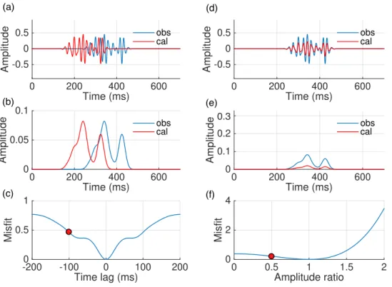
corre-spond to (a-d) in Figure 2.4, respectively. (b,e) illustrate the envelops with respect to data in (a,d), respectively. Note that the vertical axis of (f) is in logarithmic scale. For the amplitude case, the minimum is not reached for 1 due to the pre-whitening applied to the envelope. . . 52 2.8 Same as Figure 2.4, but for the envelop integral OF. (a,c,d,f) correspond

to (a–d) in Figure 2.4, respectively. (b,e) illustrate the envelop integrals with respect to data in (a,d), respectively. . . 54 2.9 Same as Figure 2.4, but for the auxiliary bump OF. (a,c,d,f) correspond

to (a–d) in Figure 2.4, respectively. (b,e) illustrate the auxiliary bump form of data in (a,d), respectively. . . 55 2.10 An illustration comparing the behavior of FWI and RWI. Sensitivity

ker-nel of FWI for a single reflector embedded in the homogeneous back-ground velocity model and its different subkernels (adapted from Chi et al., 2015): (a) full kernel of FWI, (b) transmission kernel, (c) mi-gration ellipse, (d) source-side reflection kernel, and (e) receiver-side reflection kernel. For RWI, the kernel related to macro model update includes only (d) and (e), introducing the famous rabbit ear shapes. . . . 59 2.11 CIGs related to incorrect (left) and correct (right) macro velocity models

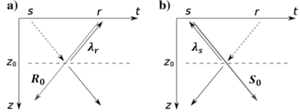
(fromChauris et al.,2002b). . . 62 2.12 Schematic view of the wavefields (a, from the source s; b, from the

re-ceiver r) contributing to the gradient in the presence of a horizontal scat-tering source (e.g. a single reflector) at depth z0 (adapted fromChauris

and Cocher, 2017). The parameters S0 and λs as well as R0 and λr

correlate between the surface and depth z0. . . 64

2.13 Description of the horizontal subsurface-offset h. . . 64 2.14 (a) CIGs and (b) associated gradients of the MVA OF computed with

classic migration for a too low (left), correct (middle), and too high (right) velocity model. Blue, white and red colors correspond to neg-ative, null and positive values, respectively (fromLameloise,2015). . . 67 2.15 Same as Figure 2.14 with a quantitative (ray-based) migration instead of

(17)

2.16 The MVA gradients for a homogeneous model with a single horizontal reflector before (a) and after (b) removing gradient artifacts by horizon-tal contraction (fromFei and Williamson,2010). . . 69 2.17 A generic workflow for solving the inverse problem in both data and

image domains (a). The differences among various approaches (b) in terms of data and model descriptions, and the criteria for the definition of OF. . . 71 3.1 Ray parameters p_s and p_r are the slowness vectors at the image point,

associated to angles θsand θr. βsand βrare oriented angles at the source

and receiver points. We define the opening angle as θ = θs− θr. . . 81

3.2 Stacked image sections obtained with migration (a, c) and inversion (b, d) for a single reflector at 0.6 km in incorrect homogeneous models, re-spectively. Compared to the exact model, the velocity is 0.5 km/s higher for (a, b) and 0.5 km/s lower for (c, d), respectively. . . 85 3.3 CIGs for position x = 2.4 km associated to images for Figure 3.2. . . . 85 3.4 Gradients obtained with classical MVA (a, d), IVA with α = 0 (b, e) and

α = 1 (c, f) for a single reflector at 0.6 km in incorrect invariant mod-els, respectively. Compared to the exact model, the velocity is 0.5 km/s higher for (a–c) and 0.5 km/s lower for (d–f), respectively. Blue, white, red colors mean negative, zero, positive values, respectively. . . 86 3.5 Same as for Figure 3.4, after the Gaussian smoothing over half a

wave-length. . . 87 3.6 (a) Exact velocity model, (b) stacked migrated section in c0 = 2.5 km/s

for all shots and (c) associated MVA gradient after a Gaussian smooth-ing over half a wavelength. From inside to outside of the Gaussian circle in panel (a), the velocity ranges from 1.6 to 2.5 km/s. Black stars and dashed line refer to shot position in panel (a). Red corresponds to posi-tive and blue to negaposi-tive value in panel (c). . . 88 3.7 For a single shot at s = 1.6 km, (a) observed data, (b) computed data

after inversion and modelling in an incorrect model of constant velocity c0 = 2.5 km/s, and (c) residuals at the same scale. Black arrows indicate

the triplicated events. . . 89 3.8 Traces extracted from Figure 3.7, for surface-offset (a) -0.5, (b) 0, and

(c) +0.5 km. The solid red line refers to the observed data and the dashed blue line to the data after inversion and modelling in an incorrect model of constant velocity c0 = 2.5 km/s. . . 90

(18)

List of Figures xv 3.9 (a) Stacked inversion section in c0 = 2.5 km/s for all shots, (b) first

gradient after a Gaussian smoothing over half a wavelength, (c) final inverted model after 10 non-linear iterations, and (d) stacked inversion section in the final model. Red corresponds to positive and blue to neg-ative value in panel (c). From inside to outside of the inverted circle in panel (c), the velocity ranges from 1.86 to 2.54 km/s. Panel (c) and Figure 3.6a are displayed with the same color scale. . . 91 3.10 CIGs associated to (a) the true Gaussian lens model, (b) the initial

homo-geneous model and (c) the updated model for position x, ranging from 0.9 to 2.7 km, every 0.3 km. Dashed black ellipses indicate the energy related to the triplication effect. Black arrows mark the same event cor-responding to different macro models. . . 92 3.11 (a) Exact velocity model and (b) observed data for a single shot at s =

1.6 km. From inside to outside of the Gaussian circle in panel (a), the velocity ranges from 1.9 to 2.5 km/s. Black stars and dashed line refer to shot position in panel (a). . . 93 3.12 Same as for Figure 3.9, but for the case displayed in Figure 3.11. From

inside to outside of the inverted circle in panel (c), the velocity ranges from 2.05 to 2.53 km/s. . . 94 3.13 Same as for Figure 3.10, but for the case displayed in Figure 3.11. . . . 95 3.14 Rays and wavefronts calculated from a source at sx = 1.6 km. (a–d)

correspond to Figures 3.6a, 3.9c, 3.11a and 3.12c, respectively. Black arrows mark the triplications. The macromodels obtained with IVA con-tain no triplications (b,d). All images are displayed with the same scale. 96 3.15 Same as for Figure 3.7, but the computed data is obtained in the correct

background model. . . 96 3.16 Same as for Figure 3.7, but the traces are extracted from Figure 3.15.

Black arrows mark the major differences between exact and reconstructed data. . . 97 3.17 Gradients obtained with classical MVA (a, b, e and f) and with IVA for

α = 1 (c, d, g and h) for the Marmousi model. The initial background velocity is a constant gradient model (from shallow to deep part: 2.0-5.0 km/s) with velocity higher than the true velocity (a, c, e and g). The initial background velocity is a 1.5 km/s homogeneous model for (b, d, f and h). Images on the right are obtained from images on the left after a Gaussian smoothing over half a wavelength distance. . . 98 3.18 Convergence curve for the IVA optimization performed on the

Mar-mousi model. The vertical axis is in logarithmic scale. Blue line rep-resents the misfit value of objective function in the iteratively updated model and red dashed line represents the cost value for the exact veloc-ity model. . . 99

(19)

3.19 True Marmousi macromodel (a) and total updated model (c0+ δc) after

100 IVA iterations (b). White stars and dashed line indicate the shot position extension. (c–f) are vertical velocity profiles at positions 2.6, 3.6, 4.6 and 5.6 km, respectively. Solid blue, dashed-dot red and solid red lines correspond to true, initial and updated macromodels, respectively.100 3.20 Stacked inverted images associated to (a) true, (b) initial and (c) updated

(Figure 3.19) macromodels, respectively. . . 101 3.21 Profiles of stacked inverted images associated with true, initial and

up-dated (Figure 3.19) macromodels. From left to right, columns are related to positions 3.0, 4.0, 5.0 and 6.0 km, respectively. Blue lines refer to im-age profiles for true model. The red lines represent profiles for initial model in the top rows and for updated model in the bottom rows. . . 102 3.22 CIGs associated to (a) the true Marmousi model, (b) the initial

homoge-neous model and (c) the updated (Figure 3.19) macromodel for position x, ranging from 2.5 to 6.5 km, every 0.5 km. We apply a taper on the image above the depth indicated by dashed black line, to exclude the associated contribution to the objective function. Black ellipse marks a local coherent event for image position (x, z) = (4.5, 1.0) km. . . 103 3.23 Single-shot inversion test in the Marmousi model: (a) observed data, (b)

inverted image, (c) reconstructed data and (d) single trace data compar-ison for trace at x = 5 km indicated by the black dashed line, respec-tively. The blue and red lines correspond to the observed and recon-structed data, respectively. . . 105 3.24 Shot gathers of (a) observed data and (b–d) modeled data for the shot at

4.6 km. Modeled data are computed for (b) true, (c) the initial and (d) the updated background models, with the associated stacked inverted images after summation over all shots. Curves in (e–g) represent the comparison between observed and modeled data for a trace at 4.6 km. The blue curves correspond to the observed data and the red dashed curves to the modeled data. The black arrow in panel (e) marks the event corresponding to the one in the ellipse in Figure 3.22. . . 106 3.25 True Marmousi full model (a) and updated model (b) after 70 FWI

iter-ations starting from the final IVA result (Figure 3.19b). (c–f) are vertical velocity profiles at positions 2.6, 3.6, 4.6 and 5.6 km, respectively. Solid blue and dashed-dot red lines represent true and updated models, respec-tively. . . 107

(20)

List of Figures xvii 3.26 Single-shot test in the Marmousi model for a shot located at 4.6 km at

the surface. (a) True reflectivity model; (b) Data modeled from (a); (c) Migrated image using the method ofQin et al.(2015); (d) Data modeled from (c); (e) Migrated image using our method; (f) Data modeled from (e). (a), (c) and (e) are plotted with the same scale. (b), (d) and (f) are all modeled in a correct smooth background model and plotted at the same scale. . . 115 3.27 Comparison between exact and reconstructed single trace data. (a–d)

are examples using the method ofQin et al.(2015). (e–h) are examples using our method. From left to right, the column refers to the single trace data located at receiver positions 2, 3, 5 or 6 km, respectively. Blue curve represents exact data. Red curve represents reconstructed data. . . 116 3.28 RMS misfit between observed and reconstructed data for each receiver

position. Blue curve represents Qin et al. (2015)’s method. Red curve represents the approach developed here. . . 116 4.1 Image-domain and data-domain IVA. Left is observed shot gather.

Mid-dle is the constructed CIG after the application of the inverse operator to the an observed data. Red, blue and greed dashed lines correspond to the cases of under-estimated, correct and over-estimated background velocity models, respectively. Right are the data modeled from the dif-ferential images in the given background velocity. Different background velocity correspond to modeled data of almost the same kinematics and they are distinguished by their amplitudes. . . 127 4.2 Stacked image sections obtained with inversion operator B†for a single

reflector at 0.6 km in different constant velocity models, respectively. Compared to the exact model, the velocity is 0.3 km/s lower for (a), equivalent for (b) and 0.3 km/s higher for (c), respectively. . . 130 4.3 CIGs for position x = 2.4 km (a–c) associated to images for Figure 4.2.

(d–f) are the residuals between adjacent traces in CIGs (a–c). Green dashed lines illustrate the curvatures of events related to different model inaccuracies. (a–c) and (d–f) are displayed with the same scale, respec-tively. . . 131 4.4 Observed data for shot position sx = 4.0 km (a), and scaling data for

shot position sx = 4.0 km (b–d) associated to image incoherency for

(d–f) in Figure 4.3, respectively. Green and black arrows correspond to the direct arrival events and the reflected events, respectively. . . 132

(21)

4.5 Gradients obtained with data-domain IVA (β = 0) for a homogeneous macromodel with velocity too low (a, d), with correct velocity (b, e) and with velocity too high (c, f), respectively. We apply the Gaussian smoothing over half a wavelength to (a–c) to derive (d–f), respectively. All images are displayed with the same scale. . . 132 4.6 Decomposition of macromodel gradients obtained with image-domain

IVA or data-domain IVA for a homogeneous macromodel with veloc-ity too low. (a) corresponds to the additional term related to α = 1 for image-domain IVA. (b–d) correspond to ˜λs? S0, ˜λr? R0and the

oscilla-tory term in equation 4.10 for image-domain IVA (α = 0), respectively. (e–h) correspond to λd ? Sd λs ? S0, λr ? R0 and the oscillatory term

in equation 4.11 for data-domain IVA (β = 0), respectively. (a–d) and (e–h) are displayed with same scale, respectively. . . 134 4.7 Gradients obtained with image-domain IVA (α = 0) (a), image-domain

IVA (α = 0) (b) and data-domain IVA (β = 0) (c) for a homogeneous macromodel with velocity too low, after a Gaussian smoothing over half a wavelength. (a) corresponds to the summation of Figures 4.6b-4.6d, (b) to the summation of Figures 4.6a-4.6d, and (c) to the summation of Figures 4.6e-4.6h. . . 134 4.8 Same as for Figure 4.6, but for a homogeneous macromodel with

veloc-ity too high. . . 135 4.9 Same as for Figure 4.7, but for a homogeneous macromodel with

veloc-ity too high. . . 135 4.10 Gradients obtained with image-domain IVA (α = 0) (a), image-domain

IVA (α = 0) (b) and data-domain IVA (β = 0) (c) with respect to the correct macro velocity model. The annihilator in all methods are replaced by the identity factor. We apply the Gaussian smoothing over half a wavelength to (a–c) to derive (d–f), respectively. (a,b,d,e) and (c,f) are displayed with the same scale, respectively. . . 136 4.11 Gradients obtained with data-domain IVA for the Marmousi model. The

initial model is a 1.5 km/s homogeneous model for (a,c,e). The initial model is a constant gradient model (from shallow to deep part: 2.0-5.0 km/s) with velocity higher than the true velocity (b,d,f). We apply the Gaussian smoothing over half a wavelength to (a,b) for (c,d) and over one wavelength for (e,f), respectively. Blue, white and red represent negative, zero and positive values, respectively. . . 137 4.12 Convergence curve for the data-domain IVA performed on the Marmousi

model. Blue line represents the misfit value of objective function for the iteratively updated model and red dashed line represents the misfit value for the exact velocity model. . . 138

(22)

List of Figures xix 4.13 Example illustrating the optimization converging towards a local

mini-mum with an improper smoothing strategy. True Marmousi background model (a) and updated model after 100 data-domain IVA iterations (b). White stars and dashed line indicate the shot position extension. (c–f) are vertical velocity profiles at positions 2.6, 3.6, 4.6 and 5.6 km, respec-tively. Solid blue, dashed-dot red and solid red lines correspond to true, initial and updated models, respectively. . . 139 4.14 True Marmousi background model (a) and updated model after 100

data-domain IVA iterations (b). White stars and dashed line indicate the shot position extension. (c–f) are vertical velocity profiles at positions 2.6, 3.6, 4.6 and 5.6 km, respectively. Solid blue, dashed-dot red and solid red lines correspond to true, initial and updated models, respectively. . . 140 4.15 Stacked inverted images associated to (a) true (Figure 4.14a), (b) initial

and (c) updated (Figure 4.14b) models, respectively. . . 142 4.16 Profiles of stacked inverted images associated with true, initial and

up-dated (Figure 4.14b) models. From left to right, columns are associated to positions 2.6, 3.6, 4.6 and 5.6 km, respectively. Blue lines refer to image profiles for true model. The red lines represent profiles for initial model in the top rows and for updated model in the bottom rows. . . 143 4.17 CIGs associated to (a) the true Marmousi model, (b) the initial

homo-geneous model and (c) the updated model (Figure 4.14b) for position x, ranging from 2.5 to 6.5 km, every 0.5 km. We apply a taper on the image above the depth indicated by dashed black line, to exclude the associated contribution to our objective. . . 144 4.18 The same as Figure 4.17, but for the image residuals computed by

com-paring adjacent traces in CIGs. All images are displayed with the same scale. . . 145 4.19 The same as Figure 4.17, but for the time-domain scaling data sets,

com-puted for shot position sx, ranging from 3.4 to 5.8 km, every 0.4 km. All

images are displayed with the same scale. . . 146 4.20 Rays and wavefronts calculated from a source at surface with sx =

6.0 km in (a) true and (b) inverted (Figure 4.14b) Marmousi macromod-els, respectively. All images are displayed with the same scale. . . 147 4.21 True Marmousi full model (a) and updated model (b) after 70 FWI

it-erations starting from the final data-domain IVA result (Figure 4.14b). (c–f) are vertical velocity profiles at positions 2.6, 3.6, 4.6 and 5.6 km, respectively. Solid blue and dashed-dot red lines represent true and up-dated models, respectively. . . 148

(23)

4.22 The first macromodel gradient, after a Gaussian smoothing over half a wavelength, obtained with image-domain IVA for α = 0 (a,e) and for α = 1 (b,f), and with data-domain IVA (c,g). (d,h) are (c,g) multiplied by the value of depth z, respectively. Compared to the exact model,the velocity is 0.5 km/s lower for (a–d) and 0.5 km/s higher for (e–h), re-spectively. . . 156 4.23 Profiles at position x = 6 km for the first gradients displayed in

Fig-ure 4.22. (a,b) are related to image-domain IVA (α = 0). In plots (c,d), solid blue, solid red and dashed red lines correspond to image-domain IVA (α = 1), and data-domain IVA before and after preconditioning, re-spectively. Compared to the exact model, the velocity is 0.5 km/s lower for (a,c) and 0.5 km/s higher for (b,d), respectively . . . 157 4.24 Profiles at x = 4.6 km extracted from background models obtained with

different methods after few nonlinear iterations. Dashed black lines cor-respond to the exact macromodel. Solid blue, solid red, and dashed red lines correspond to the results obtained with image-domain IVA (α = 1), and with data-domain IVA before and after preconditioning, respectively. The gradients for data-domain IVA is multiplied by z in (a,b), and by z2_{in (c,d). (a,c) and (b,d) correspond to the results after 1}

iteration and 2 iterations, respectively. . . 159 4.25 Macromodels obtained with different methods after 5 nonlinear

itera-tions (a) and associated CIGs (b–d). (a) is the same as Figure 4.24d, but for the case after 5 iterations. (b) is associated to the correct macro-model, and (c–e) to the results of non-preconditioned data-domain IVA, data-domain IVA preconditioned by z2 and non-preconditioned image-domain IVA, respectively. . . 160 4.26 The background model obtained after performing 100 nonlinear

itera-tions with imaged-domain IVA (a) and with data-domain IVA (b). Red arrows are at same positions for (a,b) and mark the area exhibiting dif-ferences. (c–f) are vertical velocity profiles at positions 3.5, 4.5, 5.5 and 6.5 km, respectively. Dashed black, solid blue and solid red lines correspond to true Marmousi macromodel, image-domain result (pre-conditioner z2) and data-domain result (preconditioner z2), respectively. Green arrow is at the same position as in Figure 4.28. . . 161 4.27 CIGs for starting macromodel (a,f), exact macromodel (b,e) and the

fi-nal results obtained with image-domain IVA (c,g) and data-domain IVA (d,h). (a–d) correspond to shot position 4.6 km and (f–h) to shot posi-tion 6.2 km. Dashed green rectangles are at the same locaposi-tion for (e–h) to mark the differences. . . 162 4.28 Same as for Figure 4.26, but for the results after subsequent FWI. . . 163

(24)

List of Figures xxi 5.1 Description of the impact of edge effects on macromodel gradient

ob-tained with image-domain IVA. Black dashed lines mark the boarder between well illuminated area and edges. . . 174

(25)

(26)

List of Tables

1.1 Non exhaustive review of published direct inversion approaches. For subsurface-offset and common-angle domains, the reader is referred to section 1.3.2. . . 22 3.1 Dimensions of the data, extended and shot domains. s and r are the

source and receiver coordinates, respectively. t is the time. (x,y,z) are the spatial coordinates. h is the subsurface-offset. . . 76 3.2 Non exhaustive references related to different MVA/IVA approaches. . . 78 3.3 Comparison of different approaches in terms of memory and

computa-tional requirements for calculating the gradient of the associated objec-tive function. (nz, nx) denote the size of the 2D model and ntthe sample

size of the time for the data. nh is the number of the subsurface-offset

sampling and ns the number of the shot. For a given source term, qmod

and qcross are the costs required to solve the wave equation once and to

crosscorrelate two wavefields once, respectively. . . 110 4.1 Comparison between different approaches in terms of computational

re-quirements for calculating the gradient of associated objective functions with respect to model. ns is the number of shots. For a given source

term, qmod is the CPU cost required to solve the wave equation once.

The CPU cost for crosscorrelation is neglected here. . . 129 4.2 Strategies proposed for a successful implementation of image-domain

and data-domain IVA, at least for the case of Marmousi model. . . 164

(27)

(28)

Chapter 1 Introduction

1.1 Seismic imaging principles . . . 3 1.1.1 Seismic data . . . 4 1.1.2 Scale separation . . . 6 1.1.3 Forward modeling . . . 9 1.1.4 Inverse problem . . . 10 1.2 Data-domain methods . . . 12 1.2.1 Full Waveform Inversion . . . 13 1.2.2 Linearized waveform inversion . . . 16 1.2.3 Alternative methods . . . 21 1.3 Image-domain methods . . . 24 1.3.1 Surface-oriented MVA . . . 26 1.3.2 Depth-oriented MVA . . . 28 1.4 Motivations and thesis organization . . . 29

1.4.1 Motivation I: towards common-shot inversion velocity anal-ysis – a robust approach . . . 30 1.4.2 Motivation II: investigating the link between data-domain

and image-domain methods . . . 31 1.4.3 Thesis organization . . . 32 1.4.4 Contributions . . . 34

(29)

Résumé du chapitre 1

L’imagerie sismique est très utilisée pour caractériser les structures géologiques du sous-sol au travers de l’analyse des données sismiques, pour ainsi révéler de possibles ressources souterraines. Le modèle de sub-surface est constitué de paramètres physiques comme les vitesses des ondes de pression et de cisaillement ou encore la densité des roches. Ces paramètres contrôlent la propagation des ondes dans la Terre. En raison des variations spatiales de ces paramètres, les ondes sismiques sont réfractées, réfléchies et diffractées au cours de la propagation. Des capteurs à la surface enregistrent les on-des qui ont interagit avec la sub-surface et fournissent ainsi les données pour l’imagerie sismique. Le traitement géophysique a pour objectif de convertir ces données en im-ages du sous-sol. Cette étape cruciale est formulée comme un problème inverse pour déterminer les meilleurs paramètres du modèle Terre. Un bon modèle sert ensuite pour l’interprétation géologique, la détermination des forages et le positionnement des puits. Le problème inverse est difficulté à résoudre en pratique. Parmi plusieurs raisons, la fort non-linéarité entre les données et les paramètres du modèles joue un rôle impor-tant. C’est le cas lorsque le modèle correspond aux grandes longueurs d’onde de la vitesse : un macro-modèle qui augmente de 10% ne conduit pas à un champ de pression qui change dans les mêmes proportions, mais modifie le champ d’onde complet, et en particulier les temps d’arrivées. Cette thèse ce focalise sur cette thématique.

En ce qui concerne la nature des ondes sismiques, la plupart des méthodes d’imagerie considère l’approximation acoustique avec les ondes de pression, afin de simplifier les formulations mathématiques et réduire le coût de calcul. Cette thèse est une contribu-tion à la construccontribu-tion du modèle de vitesse dans le cadre de l’approximacontribu-tion acoustique isotrope.

Dans l’introduction, je résume brièvement les principes de base autour de l’imagerie sismique dans le contexte de l’exploration géophysique, et regarde plus particulière-ment les approches classiques de la résolution du problème inverse dans les domaines des données et des images. Finalement, je motive les développements et j’explique les principales limitations actuelles des méthodes dans le domaine image et l’intérêt a faire le lien entre les domaines des données et des images.

(30)

1.1. Seismic imaging principles 3 Seismic imaging is widely used to characterize the geological structures in the sub-surface from the analysis of seismic data, and thus to reveal possible resource bear-ing formations. The subsurface model consists of a set of physical parameters such as pressure and shear wave velocities or rock density that control the wave propaga-tion in the Earth. Due to the spatial variapropaga-tions of model parameters, emitted seismic waves are refracted, reflected and diffracted during propagation. Sensors deployed at the surface record the waves traveling back to the surface after having interacted with the subsurface, to provide the data used in seismic imaging. Geophysical processing can convert those surface measurements into the images of the subsurface. This crucial step is formulated as the inverse problem aiming at determining the model parameters. An accurate subsurface model is important for subsequently interpreting the geology, determining the drilling location, and correctly positioning the wells. The inverse prob-lem, however, is difficult to solve. Among others, one reason is the highly nonlinear relationship between data and model parameters. This is the case when the model cor-responds to the large-scale part of the velocity model: a macro velocity model increased by 10% does not scale the related pressure field by the same amount, but modifies the total wavefields, including the arrival times. This thesis especially focuses on this issue. Regardless of the elastic nature of waves, most seismic imaging methods are based on acoustic assumptions and involve only pressure waves, to simplify the mathematical formulation and greatly reduce the computational cost. This thesis is a contribution related to the velocity model building under the isotropic acoustic approximation.

In this introduction, I first briefly summarize the basic principles behind seismic imaging in the context of exploration geophysics, and then pay attention to the classic approaches addressing the inverse problem defined in the data-domain or the image-domain. Finally, I motivate the research developments by explaining the main limita-tions of current image-domain methods and by indicating the interest of seeking the links between image-domain and data-domain methods.

1.1 Seismic imaging principles

In exploration geophysics, seismic experiments are widely used for the subsurface imag-ing and the reservoir management. The seismic waves can penetrate into the Earth and thus bring information about the geological structures involved in industrial production, located at a depth of a few kilometers in the subsurface. Conventional seismic explo-ration mainly takes advantage of the active seismic experiments, meaning the sources are artificially triggered, in opposition to the passive earthquake sources used in global seismology (Lay and Wallace,1995;Dahlen and Tromp,1998;Aki and Richards,2002). The passive methods, such as interferometry have also been taken into account for ex-ploration problems nowadays (Schuster et al., 2004; Schuster, 2016). In general, the study of a physical system can involve three essential elements: observed data,

(31)

for-ward modeling and inverse problem (Tarantola, 2005). In the following, I review the principles of seismic imaging for exploration problems. Additionally, I also introduce the concept of scale separation (Claerbout, 1985) distinguishing different wavenumber components of the model, as it is the basis for many seismic imaging techniques. The reader is referred toSheriff and Geldart(1995);Yilmaz(2001) for a broad introduction to seismic imaging.

1.1.1 Seismic data

Seismic data can be acquired in land and marine environments. In the land case, the source is usually a truck-mounted seismic vibrator and the receivers called geophones record the motion of particles. The receivers are typically deployed on both sides of the source at the surface (Figure1.1a). In a marine acquisition, the source is an air-gun and the receivers called hydrophones measure the pressure. The receivers are located on one side of the source, along several streamers towed by a marine seismic vessel (Fig-ure 1.1a). Alternatively, the receivers can also be located at the sea floor in an Ocean Bottom Cable configuration (MacLeod et al.,1999;Plessix and Perkins,2010). In both land and marine cases, the presence of a drilled borehole can provide a different acqui-sition system called Vertical Seismic Profiling (VSP) (Balch and Lee, 1984; Hardage,

1985; Soni, 2014). The source is similar to the one in conventional experiments but receivers are located within a well (Figure 1.1b). In the cross-well configuration, the source is a shot-hole dynamite, and sources and receivers are located in two different wells (Rector,1995;Zhou et al.,1995;Plessix et al.,2000).

A trace of seismic data is the discrete-time signal measured at a single receiver. A group of traces recorded for the same source is usually displayed on a panel called common-shot gatheror simply shot gather, with the time on the vertical axis and source-receiver distance (i.e. offset) on the horizontal axis. The shot gather records various types of structural responses to the excitated source (Figure1.2). Particular events, for example surface waves in land data and ghosts in marine data, are commonly considered as noise in seismic exploration and have to be removed by preprocessing (Yilmaz,2001), whereas global or engineering seismology may benefit from surface waves to character-ize the near-surface structure (Xia et al.,1999;Socco and Strobbia,2004;Shapiro et al.,

2005;Pérez Solano,2013). Among others, body waves are mainly considered in seismic imaging and can be categorized according to the paths that connect the source and the receiver. One group is labeled as transmitted waves, involving

• Direct wave – This type of wave travels across the superficial part of the model. The associated wave path is a straight line if the very shallow zone of the model is homogeneous;

• Diving wave – Wave-paths can be curved in the case of increasing velocities with depth. The effect may bend the waves back to the surface and the associated

(32)

1.1. Seismic imaging principles 5

(a) Surface acquisitions (taken from Danish Energy Agency)

(b) VSP acquisitions (taken from Schlumburger)

Figure 1.1 – Acquisition geometries for land and marine environments.

recording is called diving waves. Consequently, this type of waves only has a limited penetrating depth, especially for short offsets. They may arrive at the receiver with shorter time than the direct waves at large offsets;

• Refracted wave – With sharp property contrasts existing in the medium, the prop-agated waves can be refracted for the critical angles along these interfaces and then later return to the surface.

The other group is identified as scattered waves, consisting of

• First-order scattered wave – The surface excitated waves can be diffracted or re-flected when it propagates through the strong variations of medium properties. Interfaces generate reflections and sharp edges trigger diffractions. The first-order scattered waves are reflected or diffracted only once during propagation. They are

(33)

directly linked to the rapid changes of model parameters. I will focus on this type of waves in this thesis;

• High-order scattered wave – The multi-scattering is caused by strong medium property contrasts such as the sea surface or the water bottom. The energy of up-going first-scattered waves is partly sent back to the subsurface and can reflect or diffract a few times before being recorded. Their contributions are commonly ei-ther neglected or removed by the preprocessing (Verschuur et al.,1992;Verschuur,

2006). Alternatively, recent investigations propose to extend seismic imaging to multiples (Guitton,2002;Jiang et al.,2005,2007;Berkhout,2012;Verschuur and Berkhout,2015;Cocher,2017).

The preprocessing step is an essentially preliminary procedure before determining the Earth’s model parameters. It consists of selecting the interested events for the subse-quent analysis and of attenuating noise inherent to field data (seeYilmaz,2001for more details). Some developments attempt to take advantage of all information included in the data, such as transmissions, multiples, or more generally the full wavefield (see sec-tion1.2.1). However, many seismic imaging techniques still rely on primary reflection data only. In this case, the other events like multiples are considered as noise and should be removed before the further analysis. The removal of multiples is an intense research topic (Verschuur,2006). Here, the thesis only relies on the primary reflected data.

1.1.2 Scale separation

It is difficulty in practice to fully reconstruct the velocity model c with limited acquisi-tions (Virieux and Operto,2009). Conventional surface acquisition system usually pro-vides insufficient low frequencies, limited offsets and/or restricted azimuth coverage in the observed data. As demonstrated byClaerbout(1985), the model reconstructed from seismic data lacks intermediate spatial frequencies (i.e. wavenumbers). The recovered model mainly consists of two separate ranges in the spectrum (Figure 1.3), leading to the concept of scale separation that distinguishes between perturbation (high wavenum-bers) and background (low wavenumwavenum-bers) models (Jannane et al., 1989). The velocity model c is thus split into two parts,

c(x) = c0(x) + δc(x), (1.1)

where δc is the reflectivity model and c0the macro velocity or background velocity model

(Figure 1.4), according to the associated wavenumber contents. They all depend on the spatial coordinate x. The full model c can be inverted without scale separation, as in Full Waveform Inversion (FWI) presented in section 1.2.1. Alternatively, two main categories of seismic imaging methods have been established aiming at recovering different scales (Mora,1989):

(34)

1.1. Seismic imaging principles 7

reflection diving wave

refraction direct wave multiple multi diﬀraction (a) (c) (b)

Figure 1.2 – A synthetic example of marine seismic data acquired at the surface: (a) scat-tered paths in the model; (b) transmitted paths in the model; (c) shot gather recorded at the surface. The red star denotes the position of the source. Solid, dot dashed and dashed white lines in (a) denote first-reflected, multi-reflected and multi-diffracted waves, re-spectively. Solid, dot dashed and dashed white lines in (b) denote direct, diving and refracted waves, respectively.

• Migration aims at recovering the reflectivity model δc (the high-wavenumber part). Under the Born approximation, the determination of δc is a linear inverse problem. Such approaches require an accurate background velocity model c0. I

will review migration schemes in section1.2.2;

• Macro velocity estimation seeks the reconstruction of the macro velocity model c0 (the low-wavenumber part) that controls the kinematics of the recorded seismic

responses. The macro velocity model is determined with tomographic methods (in a broad sense) formulated either in the data-domain or in the image-domain (i.e. before or after migration). I will review tomographic strategies in sections1.2.3

(35)

Figure 1.3 – In black, the classic sketch byClaerbout(1985) illustrating the spatial fre-quencies that can be resolved from seismic data. The gap is now filled by the improved resolution of tomography (red curve) and by the impact of broadband acquisition on imaging (blue curve) (fromLambaré et al.,2014).

Figure 1.4 – A synthetic example of the scale separation for the Marmousi model. The full velocity model (left) is decomposed into a smooth background velocity model (mid-dle) and a velocity perturbation model (right).

In seismic imaging, it is common to deal with two types of information included in the surface measurements: the dynamic and the kinematics aspects. The dynamic aspect has a direct impact on the amplitudes of the seismic waves. It is related to the reflec-tion/transmission coefficient, but also depends on the source wavelet, the source and receiver distributions, etc. On the other hand, the kinematics of wave propagation are mainly controlled by the long-wavelength part of the velocity model, and the main con-sequence on the seismic wave is the arrival time. It also has an impact on the amplitudes due to the geometrical spreading, the attenuation in a dissipative media, etc.

Note that the spectrum gap is significantly filled nowadays (Nichols,2012;Lambaré et al.,2014) (Figure1.3): (1) the improvement of the acquisition system allows record-ing seismic data with longer offset, wider azimuth and broader frequency band; (2) the advanced imaging tools can recover the background velocity model with more details. Nevertheless, scale separation remains the theoretical basis of many conventional and new imaging methods. This thesis explicitly uses such assumption for the parameteri-zation of the model.

(36)

1.1. Seismic imaging principles 9 Before discussing data-domain and image-domain methods, I first review the main elements in forward modeling and in the resolution of the inverse problem.

1.1.3 Forward modeling

For subsequent imaging procedures, it is essential to define a physical law that allows to properly describe the link between the chosen model parameters and the associated data. It is mathematically formulated as a hyperbolic partial differential equation called wave equation, which simulates the wave propagation giving a set of model parameters. In the real Earth, the wave propagation is affected by many subsurface properties. Due to the high computational cost of simulating the visco-elastic anisotropic wave propa-gation, I consider only the isotropic acoustic approximation in this thesis. Anisotropy, elasticity and attenuation are not included. The Earth’s model is thus paramterized by the pressure wave velocity Vpand the rock density ρ. The reflections are generated from

rapid changes of acoustic impedance Ip = Vpρ. In the constant density case, only the

pressure wave velocity needs to be specified to solve the wave equation. Even for this simplest assumption, one still has to input a large number of parameters since the model parameters depend on the spatial coordinates.

The wave equation is commonly resolved by numerical modeling schemes including finite-difference method (FDM) (Virieux, 1986; Levander, 1988; Etgen and O’Brien,

2007), finite-element method (FEM) (Smith, 1975; Marfurt, 1984), spectrum-element method (SEM) (Komatitsch and Vilotte,1998;Komatitsch and Tromp,1999), etc. In ex-ploration geophysics, the two main forward modeling tools are FDM and FEM.Moczo et al. (2010, 2011) compared the two schemes and concluded that the accuracy of the two methods are comparable with fine samplings. Virieux et al.(2011) have reviewed the efficiency and complexity of the two methods, and indicated that FDM is widely used due to its simplicity to implement and the relatively lower computational cost. The main advantage of FEM is its flexibility in meshing to deal with the boundary condi-tions and irregular structures. Compared to FDM, it is more numerically expensive and more difficult to implement. SEM is more applied for global seismology scale problems (Komatitsch and Vilotte, 1998; Komatitsch and Tromp, 1999; Fichtner, 2011). Some investigations proposed to use SEM on the exploration scale (Luo et al., 2009, 2013), but SEM is very demanding in terms of the computational cost and its grid meshing requires a priori knowledge of the subsurface structure. This thesis will concentrate on simulating the wavefield with FDM.

The modeling can also rely on the ray theory, which is based on the high-frequency asymptotic approximation of the wave equation (Cervenýˇ , 2005). The propagation of waves in the subsurface is described by rays sharing the similar propagation laws used in optics (Cervený et al.ˇ ,1977;Chapman,2004). For this scheme, the Green’s function can be decomposed into three parts: one corresponding to the traveltime, one to the amplitude and one to the source signature. In a given velocity model, the traveltime can

(37)

be simulated either by ray-tracing strategy (Julian,1977;Cerven`yˇ ,1987), or by solving the Eikonal equation (Vidale,1988;Podvin and Lecomte,1991;Qin et al.,1992).

In this thesis, I only focus on wave-equation-based modeling methods (in particular FDM) and ray-based modeling methods will not be considered, except for analyzing the main effects of wave-equation operators on the data.

1.1.4 Inverse problem

Objective function

The inverse problem consists of defining a scalar objective function (also called cost function) to evaluate the accuracy of model parameters used for modeling. It is de-signed such that the best model corresponds to the global maximum or minimum in the objective function. In the data-domain, the objective functions can be defined by mea-suring the misfit between observed and modeled data, typically in the least-squares sense (Tarantola, 1984a;Pratt et al.,1998). Alternatively, the data misfit can also be assessed using other schemes such as crosscorrelation (Luo and Schuster, 1991; Van Leeuwen and Mulder,2010), deconvolution (Luo and Sava,2011;Warner and Guasch,2016), op-timal transport distance (Métivier et al.,2016), Huber norm (Guitton and Symes,2003), etc. On the other hand, one can first migrate the data and then formulates the objective functions in the image-domain, with semblance principle (see section 1.3 for details), measuring the level of coherency or focusing of reconstructed reflectivity images of the Earth (Al-Yahya, 1989; Symes and Carazzone, 1991; Sava and Biondi, 2004; Symes,

2008).

In seismic imaging, the inverse problem generally seeks a set of model parame-ters minimizing the objective function. However, it is in practice an ill-posed problem (Tarantola, 1984a; Scales et al., 1990;Virieux and Operto, 2009). The solution is not unique, meaning that there are probably several models that can perfectly explain the data for a given noise level. Some regularizations are conventionally applied to make the inverse problem better posed (Tikhonov et al., 1977; Menke, 1984;Hansen, 2000;

Asnaashari et al., 2013). The non-uniqueness problem results from various reasons in-cluding the imperfect acquisition and the crosstalk among different physical parameters (Tarantola,2005). Most of the seismic surveys are located at the surface of the Earth and the offsets are limited, leading to insufficient illumination of the subsurface, especially in the area with complex geological structures (e.g. salt body and gas clouds). Conse-quently, some of the subsurface model parameters may be poorly or even not sampled, such that they cannot be retrieved by analyzing the measurements. For example, the lo-cal change of seismic velocity and attenuation property may produce similar reflection coefficients (Mulder and Hak, 2009; Hak and Mulder, 2010). To reduce the crosstalk, a proper parameterization is needed, for which the model parameters are less coupled (Virieux and Operto,2009;Zhou et al.,2015;He and Plessix,2017).

(38)

1.1. Seismic imaging principles 11 Optimization scheme

Inverse problem aims at determining a set of model parameters minimizing the objective function through an optimization procedure. One possible solution is the global opti-mization methods (also called the global search methods) (Sen and Stoffa,2013), which explore the whole model space to determine the optimum choice. Such schemes require the ability to calculate the value of the objective function and to properly sample the model space. For example, Monte Carlo methods (Jin and Madariaga,1994;Sambridge and Mosegaard,2002), simulated annealing (Ingber,1989;Mosegaard and Vestergaard,

1991; Scales et al., 1992; Misra and Sacchi, 2008) and generic algorithms (Gallagher et al., 1991; Sambridge and Drijkoningen, 1992; Jin and Madariaga, 1993) have been applied to the geophysical inverse problems. The main limitation of these schemes is the computational cost because they require evaluating the objective functions numerous times.

On the other hand, a realistic alternative is the local optimization methods (also called gradient-based methods), applicable if the objective function does not contain local minima. Examples of this family are steepest descent methods (Lines and Treitel,

1984; Tarantola, 1984a), nonlinear conjugate gradient methods (Fletcher and Reeves,

1964; Portniaguine and Zhdanov, 1999; Luo and Schuster, 1991), Gaussian-Newton methods (Shin,1988), quasi-Newton methods (Nocedal,1980;Nash and Nocedal,1991) and Newton methods (Santosa et al., 1987; Pratt et al., 1998; Métivier et al., 2013). For these schemes, the model is iteratively updated such that the value of the objective function decreases with iterations (Figure1.5). The direction of the model update at each iteration is determined by calculating the gradient of the objective function with respect to model parameters, and possibly the inverse of the Hessian to take into account the local curvature of the objective function. The adjoint-state technique (Chavent, 1974;

Plessix,2006) provides an efficient way to derive of the gradient of the objective function with respect to model parameters.

(39)

The nonlinear relationship between data and model parameters is an intrinsic dif-ficulty for the local optimization procedure: the objective function is not necessarily convex and it may converge towards a local minimum instead of the global one (Bunks et al., 1995). Therefore, it is important to start from an initial model close enough to the true model (Beydoun and Tarantola, 1988; Pratt et al., 2008). The alternative is to develop a multi-scale approach and to start with the low-frequency content of the data. The presence of low-frequency content in the observed data can relax the requirement for the initial model (Sirgue, 2006): for example, the classical least-squares objective function has an enlarged basin of attraction. I will explain the nonlinear issues more in section 1.2.1. Strategies to define the objective functions with better convex property will be reviewed in sections1.2.3and1.3.

I have reviewed the seismic imaging principle in this section. In the following sec-tion, I review the inverse problems formulated in data-domain and image-domain, as I will investigate the links between two families later in Chapter 4. Although mod-eling aspects with ray theory were reviewed in section 1.1.3, I will only investigate the wave-equation-based methods in the following Chapters, except for analyzing the wave-equation operators. The rays can emphasize the kinematics of wave propagation in the subsurface. However, ray-based methods poorly behave for sampling the shadow zone (a low velocity anomaly area) (Moser, 1991). Ray-based methods have built-in disadvantages including the limited resolution of recovered model (a ray travels trough a infinitesimally narrow path inside the model) and the instability dealing with strong heterogeneities (Díaz et al., 2014; Wang et al., 2014). I now detail the classic inverse problems defined in the data-domain, and the principle of image-domain techniques will be reviewed in section1.3. Note that a tomographic mode corresponds to the update of macromodel c0 and a migration mode to the update of model perturbation δc as

men-tioned in section1.1.2.

1.2 Data-domain methods

The data-domain methods measure the misfit between observed and modeled data to evaluate the quality of an estimated model (Tarantola,2005). Under the isotropic acous-tic approximation, the model c corresponds to the pressure wave velocity field. In sec-tion 1.2.1, I first review the FWI strategy, which uses the full recorded data to recon-struct c without any scale separation. Then, in section 1.2.2, I introduce the migration technique as a linearized waveform inversion problem. The method relies on the scale separation assumption and is dedicated to recovering the small scale structure δc. The reconstruction of the background model c0 is challenging. Traveltime tomography has

becomes a standard for estimating the macro velocity model c0in the oil and gas industry