HAL Id: hal-01800804
https://hal.archives-ouvertes.fr/hal-01800804
Preprint submitted on 28 May 2018
HAL is a multi-disciplinary open access
archive for the deposit and dissemination of
sci-entific research documents, whether they are
pub-lished or not. The documents may come from
teaching and research institutions in France or
abroad, or from public or private research centers.
L’archive ouverte pluridisciplinaire HAL, est
destinée au dépôt et à la diffusion de documents
scientifiques de niveau recherche, publiés ou non,
émanant des établissements d’enseignement et de
recherche français ou étrangers, des laboratoires
publics ou privés.
Complexity of parallel scheduling unit-time jobs with
in-tree precedence constraints while minimizing the
mean flow time
Tiayu Wang, Odile Bellenguez-Morineau
To cite this version:
Tiayu Wang, Odile Bellenguez-Morineau. Complexity of parallel scheduling unit-time jobs with in-tree
precedence constraints while minimizing the mean flow time. 2018. �hal-01800804�
(will be inserted by the editor)
Complexity of parallel
scheduling unit-time jobs with
in-tree precedence constraints
while minimizing the mean
flow time
Tianyu Wang · Odile Bellenguez-Morineau
Received: date / Accepted: date
Abstract This paper deals with a particular schedul-ing problem. We consider unit-time jobs and in-tree precedence constraints while minimizing the mean flow time. This problem is observed as P |pj= 1, in-tree|P Cj
with the use of the 3-filed notation. To the best of our knowledge, its complexity is still open. Through a re-duction from 3-Partition, we show that this problem is N P-complete.
Keywords parallel scheduling · in-tree · precedence constraints · complexity theory
Acknowledgments
This work was supported by the China Scholarship Coun-cil [grant numbers 201404490037].
1 Introduction
We consider the following scheduling problem: a set of n unit-time jobs (pj = 1) has to be done by m identical
parallel machines. The jobs are submitted to precedence constraints. Prot and Bellenguez-Morineau (2018) re-vealed the fact that the complexity of a problem is likely
Tianyu Wang
Institut Mines-T´el´ecom Atlantique, LS2N, UMR CNRS 6004, 4 rue Alfred Kastler, B.P. 20722 F-44307 Nantes Cedex 3. France
Tel. +33 7 82 99 22 36 E-mail: [email protected] Odile Bellenguez-Morineau
Institut Mines-T´el´ecom Atlantique, LS2N, UMR CNRS 6004, 4 rue Alfred Kastler, B.P. 20722 F-44307 Nantes Cedex 3. France
E-mail: [email protected]
to be different for specific type of precedence graphs. In this paper, we focus on the problem with in-trees (or in-forest in some literature) precedence graph. This particular graph suggests that each job has no more than one successor. We use Cjto denote the completion
time of a job j. The problem involves finding an opti-mal schedule, respecting the precedence constraints and minimizing the total completion timeP Cj. This
crite-rion is termed as mean flow time(noted as MFT in the following text). When the number of machines m is not fixed, this problem is noted as P |pj = 1, in-tree|P Cj
in the 3-field notation of Graham et al. (1979). This problem was among the minimal open prob-lems according to Sigrid Knust (2009). To the best of our knowledge, it is still open (Prot and Bellenguez-Morineau, 2018). Herein, we aim at providing a proof of its N P-completeness.
Organization of this paper is as hereunder: in the subsequent section, we present the state of the art. In section 3, we prove that the problem P |pj= 1, in-tree|P Cj
is N P-complete. In subsection 3.1, we present how we reduce the 3-Partition problem to the decision ver-sion of the scheduling problem. We prove the N P-completeness in detail in subsection 3.2 and 3.3. Finally, section 4 provides our conclusion.
2 State of the art
A study involving in-tree precedence constraints in a parallel machine scheduling problem has been performed: Hu (1961) focus on the makespan and suggests that the problem is polynomially solvable using the HLF(highest level first) strategy. Nevertheless, Garey et al. (1983) prove that the problem is N P-complete when the prece-dence graph is an opposing forest, which corresponds to a set of in-trees and out-trees.
HLF can also be used to minimize the MFT if the precedence graph is an out-tree. Furthermore, a polyno-mial algorithm is put forward by Brucker et al. (2001) for the solution of this problem in case of allowance of preemption.
Nevertheless, Huo and Leung (2006) show HLF can-not optimally solve the in-tree version. In addition, Bap-tiste et al. (2004) proved that it can be solved in O(nm)
time, i.e. if the number of machines m is a fixed param-eter, the problem is polynomially solvable.
Finally, Garey et al. (1983) prove that the prob-lem is N P-complete for a profile scheduling. Accord-ingly, the number of available machines varies along the time rather than parallel machines. However, the com-plexity of the given parallel scheduling problem P |pj=
2 Tianyu Wang, Odile Bellenguez-Morineau
3 Proof of N P-completeness
In a bid to prove N P-completeness of P |pj = 1, in-tree|P Cj,
we employed a reduction from a known N P-complete problem: 3-Partition. An instance π1of the 3-Partition
problem (noted Π1) is defined as hereunder (Garey and
Johnson, 2002):
Definition 1. Let α be a set of 3q elements and B an integer, we have ∀a ∈ α, ∃wa∈ Z+, B4 < wa< B2 and
P
a∈α
wa= qB. The question is: is there a partition of α,
which is α1, α2, . . . , αq, such that ∀i ≤ q, P a∈αi
wa = B
?
As Π1is N P-complete in the strong sense, the
theo-rem provided hereunder allows us to employ a pseudo-polynomial transformation(Garey and Johnson, 2002, p. 101):
Theorem 1. If Π is N P-complete in the strong sense, Π0 ∈N P and there exists a pseudo-polynomial transfor-mation from Π to Π0, then Π0 is N P-complete in the strong sense.
Firstly, we define Π2 as P |pj = 1, in − tree|P Cj ≤
M F T∗, which represents the decision version of our scheduling problem. The decision question deals with whether there exists a feasible schedule such thatP Cj≤
M F T∗ or not, where M F T∗ is a given integer. In the subsequent part, we demonstrate how to reduce any in-stance π1 of Π1 to an instance π2of Π2.
3.1 Transformation
In order to begin our transformation, we define some constants:
– B = q5B
– ∀a ∈ α, wa = q5wa
– K = B5
– m = 3q + 1 + B, which will be used as the number of machines – M F T∗= q P i=1 i(3(q + 1 − i) + 1) + K3 P i=q+1 i + B q P i=1 i + P a∈α Kwa P i=1 i + KB q P i=1 i – ∀k ≤ q + 1, mk = B + 3k − 3
Notice that an optimal partition for π1, such that
P
a∈αi
wa = B, is totally equivalent to a partition such
that P
a∈αi
wa = B , since the problem does not change when multiplying wa by an integer q5.
Thereafter, we create the following jobs:
u
1 au
2au
3au
wa av
1 av
2 av
3 av
4av
5 av
Kwa aFig. 1: in-tree of u-jobs and v-jobs
– For each a ∈ α, we build two sets of jobs, which in-clude u-jobs and v-jobs: u1
a, u2a, . . . , uwaa, and va1, v2a, . . . , vaKwa.
The u-jobs precede directly v1
a, i.e. ∀i ≤ wa, uia≺ v1a.
Subsequent to that, we set vai ≺ vi+1a , ∀i < Kwa,
and they form a chain. The corresponding tree of the u-jobs and v-jobs can be observed in the Figure 1. They form 3q in-trees
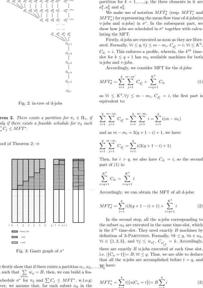
– In addition, we consider a set of d-jobs, which are defined as hereunder: d11, . . . , dm−m1 1 d12, . . . , d m−m2 2 . . . d1q, d2q, d3q, d4q dq+1 dq+2 . . . dK3
Those d-jobs also design a tree. In that tree, we fix for any k ≤ q + 1, d1
k−1 ≺ d1k, d2k−1 ≺ d1k and d3k−1 ≺ d1 k. ∀i ∈ {4, 5, . . . , m − mk−1}, then, we set: di k−1 ≺ d i−3 k . Thereafter, for ∀k ∈ {q + 2, q + 3, . . . , K3}, d
k−1≺ dk, accordingly forming a chain.
The corresponding tree is presented in the Figure 2. Thus, we transformed π1 to an instance π2 of the
scheduling problem Π2. The construction is made in
polynomial time of B and q (pseudo-polynomial). In accordance to the Theorem 1, we can establish the N P-completeness of Π2 through the provision of theorem
d1 1 d21 d31 d41 d51 d61 d71 d81 d91d101 d m−m1 1 d1 2 d22 d32 d42 d52 d62 d72 dm−m2 2 d1 3 d22 d32 d42 d m−m3 3 d4 q d1 q dq+1 dq+2 dq+3 dq+4 dq+5 dK3 d3 q d2 q ... ... ... ...
Fig. 2: in-tree of d-jobs
Theorem 2. There exists a partition for π1 ∈ Π1, if
and only if there exists a feasible schedule for π2 such
that P Cj≤ M F T∗. 3.2 Proof of Theorem 2: ⇒ 0 1 2 3 4 q − 1 q q + 1 t 5 6 dummy jobs v-jobs u-jobs
Fig. 3: Gantt graph of σ∗
We firstly show that if there exists a partition α1, α2, . . . , αq
for π1, such that P a∈αi
wa= B , then, we can build a
fea-sible schedule σ∗ for π2 and P Cj ≤ M F T∗. w.l.o.g:
moreover, we assume that, for each subset αk in the
partition for k = 1, . . . , q, the three elements in it are ak
1, ak2 and ak3.
We make use of notation M F Td∗ (resp. M F Tv∗ and M F Tu∗) for representing the mean flow time of d-jobs(resp. v-jobs and u-jobs) in σ∗. In the subsequent part, we show how jobs are scheduled in σ∗ together with calcu-lating the MFT.
Firstly, d-jobs are executed as soon as they are liber-ated. Formally, ∀i ≤ q, ∀j ≤ m − mi, Cdji = i; ∀i ≤ K
3,
Cdi = i. This enforces a profile, wherein, the k
th
time-slot for k ≤ q + 1 has mk available machines for both
u-jobs and v-jobs.
Accordingly, we consider MFT for the d-jobs:
M F Td∗= q X i=1 m−mi X j=1 Cdj i + K3 X i=q+1 Cdi (1) as ∀i ≤ K3, ∀j ≤ m − m
i, Cdji = i, the first part is
equivalent to: q X i=1 m−mi X j=1 Cdj i = q X i=1 m−mi X j=1 i = q X i=1 i(m − mi) and as m − mi= 3(q + 1 − i) + 1, we have: q X i=1 m−mi X j=1 Cdj i = q X i=1 i(3(q + 1 − i) + 1)
Then, for i > q, we also have Cdi = i, so the second
part of (1) is: K3 X i=q+1 Cdi= K3 X i=q+1 i
Accordingly, we can obtain the MFT of all d-jobs:
M F Td∗= q X i=1 i(3(q + 1 − i) + 1) + K3 X i=q+1 i (2)
In the second step, all the u-jobs corresponding to the subset αk are executed in the same time-slot, which
is the kth time-slot. They need exactly B machines by definition of 3-Partition. Formally, ∀k ≤ q, ∀a ∈ αk,
∀i ∈ {1, 2, 3}, and ∀j ≤ wak i, Cujak
i
= k. Accordingly, there are exactly B u-jobs executed at each time slot, i.e. |{Cu= t}|= B, ∀t ≤ q. Thus, we are able to deduce
that all the u-jobs are accomplished before t = q, and we have: M F Tu∗= q X t=1 t|{u|Cu= t}|= B q X i=1 i (3)
4 Tianyu Wang, Odile Bellenguez-Morineau
Thereafter, every v-job is executed without any de-lay in accordance with the precedence constraints. For-mally, ∀a ∈ α, Cv1
a= Cu1a+ 1 and ∀i ∈ {2, 3, . . . , Kwa},
Cvi
a= Cvi−1a + 1.
So, for each v-chain corresponding to the element a ∈ α, we have Cvi
a = Cvi−1a + 1, ∀i ∈ {2, 3, . . . , Kwa},
that is Cvi
a= Cva1+ i − 1. Let uabe any u-job preceding
va1, as Cv1
a= Cua+ 1, we have Cvia= Cua+ i. Now, we
calculate the MFT for this given chain:
Kwa X i=1 Cvi a = Kwa X i=1 Cua+ Kwa X i=1 i = KwaCua+ Kwa X i=1 i
Then, we deduce the MFT for all these v-chains, i.e. all the v-jobs:
M F Tv∗= X ∀a∈α Kwa X i=1 Cvi a = K X ∀a∈α waCua+ X ∀a∈α Kwa X i=1 i
We are aware of the fact that, for each subset αk, we
have Cuai
j
= i, where j ∈ {1, 2, 3}, and i ≤ q. So, we are able to deduce that the first part is equivalent to:
K X ∀a∈α wa X j≤wa Cuj a = K q X i=1 X ∀a∈αi wa X j≤wa Cuj a= K q X i=1 i X ∀a∈αi wa= K q X i=1 iB So, M F Tv∗= K q X i=1 iB + X ∀a∈α Kwa X i=1 i (4)
So, in kthtime slot of σ∗, k < q +1, there are exactly
m−mkd-jobs, B v-jobs and 3k −3 v-jobs. By definition
of mk, there are exactly m jobs in progress. After t = q,
there are only one d-job and at most 3q v-jobs executed in parallel. Thus, there are no more than m jobs. So, this schedule respects the availability of machines.
Then, we deduce that the total MFT of σ∗, which
is a feasible schedule for π2, is:
X
Cj= M F Tv∗+ M F Tu∗+ M F Td∗= M F T∗
3.3 Proof of Theorem 2: ⇐
In this section, we prove that if π2 has a feasible
sched-ule, then π1 has a partition. A schedule without
un-forced idle time is termed as non-delay schedule by Weiss and Pinedo (2012). The authors also prove that there always exists an optimal non-delay schedule. Let σ be a feasible non-delay schedule. We prove in the
following part that σ takes the same shape as σ∗ and followed by building a partition from σ.
For that purpose, we at first, define the MFT of u-jobs, v-jobs and d-jobs in σ as M F Tu, M F Tv and
M F Td. Subsequent to that, define the following gaps:
∆u= M F Tu− M F Tu∗
∆v= M F Tv− M F Tv∗
∆d= M F Td− M F Td∗
In order to respect the M F T∗, we understand that: ∆d+ ∆u+ ∆v ≤ 0 (5)
In addition to this, we would like to throw emphasis on the following observations:
Observation 1. When a chain of nc jobs is
right-shifted by one time slot, then its MFT will be increased by nc.
Observation 2. The sizes of different sets of jobs ex-hibit the following relation:
K3 Kwa B q5
First of all, let us consider the d-jobs. We show that d-jobs must have the same profile as in σ∗, which is the following lemma:
Lemma 1. In σ, the d-jobs are scheduled as soon as they are liberated (as in σ∗), i.e. ∆
d= 0.
Proof. By contradiction: assume that there is at least one delayed d-job. σ is a non-delay schedule; accord-ingly, this d-jobs can be delayed only by insertion of u-jobs or v-jobs.
Notice that the d-jobs can take no more than m−m1
machines in parallel because of the precedence con-straints. At any moment, there are at least m1 = B
available machines for both the v-jobs and u-jobs. More-over, in a non-delay schedule, the makespan(Cmax) is
not larger than the number of jobs. As the total number of v-jobs and u-jobs is KB + qB, the last v-job or u-job finishes before KB + qB. Consequently, the delay must happen before KB + qB.
As the length of the d-chain is K3, at least K3− KB + qB jobs are right-shifted. Following the Observa-tion 1, we have ∆d≥ K3− KB + qB Remind that M F Tu∗ K2, M F T∗ v K2, so we have ∆d M F Tu∗+ M F T ∗ v
In accordance with the definition, we have ∆u > −M F T∗ u and ∆v> −M F Tv∗, then ∆d+ ∆v+ ∆u > ∆d− M F Tu∗− M F T ∗ v 0
This is a contradiction to (5). So, our assumption is false, there is no delay during the execution of d-jobs.
Since ∆d= 0, (5) becomes
∆u+ ∆v≤ 0 (6)
Here we conclude that the profile of available ma-chines in σ is the same as in σ∗ to schedule u-jobs and
v-jobs. Now, let us deal with u-jobs.
Definition 2. We define the u-jobs in the same com-ponent a u-set and define Ut as the number of u-jobs
in u-sets completed at t.
Lemma 2. At time t∗ ≤ q, the completed u-sets con-tain at most t∗B u-jobs, i.e.
t∗
P
t=1
Ut≤ t∗B.
Proof. The number of jobs finished at t∗≤ q is at most t∗m which is:
t∗m = t∗B + t∗(3q + 1) ≤ t∗B + 3q3
As we are aware of the fact, the number of u-jobs in a u-set is wa, which is integer times q5, so, the number of
u-jobs in completed u-sets is at most t∗B. Now, let us move on to the v-jobs.
Definition 3. We define Vtas the number of v-jobs in
the chains starting at the time t for t < q in σ, and Vq as the number of v-jobs in the chains starting at or
after t = q.
Lemma 3. In σ, at any time t ≤ q, the total length of the v-chains beginning at t in σ is exactly KB, as in σ∗, i.e. Vt= KB.
Proof. At first, we prove that
q P i=1 iVi≥ KB q P i=1 i. According to the precedence constraints, we have a relation between Vt and Ut:
t∗ X t=1 Vt≤ K t∗ X t=1 Ut ∀t∗< q
So, from Lemma 2, we can deduce:
t∗ X t=1 Vt≤ t∗BK ∀t∗< q which is: (7) V1≤ KB V1+ V2≤ 2KB V1+ V2+ V3≤ 3KB . . . . . . V1+ V2+ V3+ · · · + Vq−1≤ (q − 1)KB
If we sum them up, we get:
(q − 1)V1+ (q − 2)V2+ · · · + Vq−1≤ KB
q2− q
2 (8) By definition, we understand that Pq
t=1Vt
corre-sponds to the norm of whole set of v-jobs and it is equal to KqB:
q
X
t=1
Vt= KqB (9)
Then, by multiplying (9) by q, we get:
qV1+ qV2+ . . . qVq = KBq2 (10) With (10)-(8), we get V1+ 2V2+ · · · + (q − 1)Vq−1+ qVq≥ KB q2+ q 2 which is exactly q X i=1 iVi≥ KB q X i=1 i
It requires observation that the two terms are equal if and only if every decomposition of group (7) is written with an equality, which indicates that V1= V2= · · · =
Vq= KB.
Now, we demonstrate that
q P i=1 iVi= KB q P i=1 i. Sup-pose by absurd that
q P i=1 iVi > KB q P i=1 i. By definition, Vi is the total length of some v-chains, which implies
that Vi is integer times K. So, we have: q X i=1 iVi≥ KB q X i=1 i + K (11)
In the best case of σ, all the v-jobs in one chain are executed without any delay, so, we have:
M F Tv ≥ X a∈α Kwa X i=1 i + q X i=1 iVi (12)
Reminding the expression of M F Tv∗ in (4), we can de-duce that: ∆v≥ q X i=1 iVi− KB q X i=1 i (13)
6 Tianyu Wang, Odile Bellenguez-Morineau
By (13) and (11), we have∆v≥ K. Then, by (6), we
have ∆u ≤ −K. This contradicts the fact that ∆u ≥
−M F T∗
u −K.
Finally, we can conclude that ∆v= 0 and Vt= KB,
∀t ≤ q. This suggests that, at any t, the length of v-chains started is exactly KB.
The Lemma above allows us to build a partition from Vi by selecting the elements corresponding to its
3 v-chains of KB jobs. Thus, we accomplished the proof for the Theorem 2.
4 Conclusion
In this paper, we put forward a proof of N P-completeness for P |pj= 1, in-tree|P Cj. Based on that, we refine the
knowledge about the complexity of parallel scheduling problems subjected to precedence constraints in specific graphs.
Nevertheless, some open problems still exist requir-ing investigation. For example, when preemption is
al-lowed, the complexity of the problem P |pj= 1, in-tree, pmtn|P Cj
is unknown. We conjecture that, with the same reduc-tion as in subsecreduc-tion 3.1, the Theorem 2 still holds even if preemption is allowed, and the problem shall be N P-complete as well.
Another possible research avenue involves exploration of how to solve the problem when m is a fixed number. The complexity of the algorithm proposed by Baptiste et al. (2004) is O(nm), but it can be certainly improved.
References
Philippe Baptiste, Peter Brucker, Sigrid Knust, and Vadim G Timkovsky. Ten notes on equal-processing-time scheduling. Quarterly Journal of the Belgian, French and Italian Operations Research Societies, 2 (2):111–127, 2004.
Peter Brucker, Johann L Hurink, and Sigrid Knust. A polynomial algorithm for P |pj= 1, rj, outtree|P Cj.
Math. Methods Oper. Res., 2001.
Michael R Garey and David S Johnson. Computers and intractability, volume 29. wh freeman New York, 2002.
MR Garey, DS Johnson, RE Tarjan, and Yannakakis M. Scheduling opposing forests. SIAM Journal on Algebraic Discrete Methods, 4(1):72–93, 1983. Ronald L Graham, Eugene L Lawler, Jan Karel
Lenstra, and AHG Rinnooy Kan. Optimization and approximation in deterministic sequencing and scheduling: a surveyhaha. Annals of discrete mathe-matics, 5:287–326, 1979.
Te C Hu. Parallel sequencing and assembly line prob-lems. Operations research, 9(6):841–848, 1961. Yumei Huo and Joseph Y-T Leung. Minimizing mean
flow time for UET tasks. ACM Transactions on Al-gorithms (TALG), 2(2):244–262, 2006.
Damien Prot and Odile Bellenguez-Morineau. A survey on how the structure of precedence constraints may change the complexity class of scheduling problems. Journal of Scheduling, 21(1):3–16, 2018.
Peter Brucker Sigrid Knust. Complex-ity results for scheduling problems, 2009. http://www2.informatik.uni-osnabrueck.de/knust/class/.
Gideon Weiss and Michael Pinedo. Scheduling: Theory, algorithms, and systems, 2012.