HAL Id: hal-02280012
https://hal.archives-ouvertes.fr/hal-02280012
Submitted on 5 Sep 2019
HAL is a multi-disciplinary open access
archive for the deposit and dissemination of
sci-entific research documents, whether they are
pub-lished or not. The documents may come from
teaching and research institutions in France or
abroad, or from public or private research centers.
L’archive ouverte pluridisciplinaire HAL, est
destinée au dépôt et à la diffusion de documents
scientifiques de niveau recherche, publiés ou non,
émanant des établissements d’enseignement et de
recherche français ou étrangers, des laboratoires
publics ou privés.
Distributed under a Creative Commons Attribution| 4.0 International License
adaptation
R Pethe, T Heuze, L. Stainier
To cite this version:
R Pethe, T Heuze, L. Stainier. Variational Approach for thermo-mechanical mesh adaptation. 22e
Congrès Français de Mécanique, Aug 2015, Lyon, France. �hal-02280012�
Variational Approach for
thermo-mechanical mesh adaptation
R. PETHE
1, T. HEUZE
1, L. STAINIER
1 1. GeM, Ecole Centrale de Nantes,{pethe.rohit,thomas.heuze,laurent.stainier}@ec-nantes.fr
Abstract
In this work, we study the variational approach to mesh adaptation. This approach is shown on a 1-D thermal problem in steady case. The solution obtained with an adapted mesh is compared to that computed with a uniform refinement. We demonstrate that variational mesh adaptation technique costs less than taking a uniform mesh when precise solution is needed.
Keywords : variational, mesh adaptation, thermo-mechanical
1 Introduction
In many engineering problems (thermal or structural), zones of high gradient of fields of interest evolve with time and loading. When we solve such a problem with finite elements method, mesh has to be dynamically adapted in order to capture solution in zones of high gradients with required precision.
Many methods of mesh adaptation are proposed in the literature based on error estimators. But, these methods have limitations when we wish to treat problems with non-linear constitutive relations (e.g. plasticity).
An alternative approach of mesh adaptation was recently proposed [1] [2] based on variational approach [3]. This technique allows to perform calculations in the presence of large transformations and nonlinear irreversible behavior (e.g. plasticity).
In this work, we are focusing on steady state thermal problems. In this case, we try to minimize energy like potential Φ. Firstly, we calculate the finite element solution on initial mesh. Secondly, on each element, we calculate the local value of energy like potential. Thirdly, we add a node in middle of the element. fourthly, we solve local problem on the element by fixing the temperature at end nodes. (Therefore, it becomes a 1D problem.) Then, we check if we improve significantly the energy like potential locally by adding this node. If we do, we add this node in the global mesh. Finally, we solve whole problem again on the new mesh obtained. We repeat the procedure till we get a solution of required precision.
2 Variational Formulation
The solution for steady thermal problem is found my minimizing the following con-vex potential: φ(T (x)) = Z Ω 1 2k −−→ gradT ·−−→gradT dΩ − Z Ω rT dΩ (1)
where k is the thermal conductivity, r the internal heat source, T the temperature field and Ω the domain. If we are dealing in 1D, the strong form reads:
kd 2T
dx2 + r = 0 (2)
with boundary conditions:
T (x = 0) = T 0 T (x = L) = T 1
(3)
3 Applications
Now, we try to apply this theory to thermal stationary problem. (The transient prob-lem will be presented during the conference.)
3.1 Analytical Solution
The equation to be solved in stationary problem can be represented as follows: kd
2T
dx2 + r = 0 (4)
with boundary conditions:
T (x = 0) = T 0 T (x = L) = T 1
(5) Here, k is the thermal conductivity of the material, T is the temperature field, r is
the internal heat generation, L is the length of the rod, and q is a constant. We take,
r = xq T 0 = 0 T 1 = 0
(6) Therefore, the analytical solution of the problem can be given as follows:
T = L
q+1x (q + 1)(q + 2)−
xq+2
(q + 1)(q + 2) (7)
The energy potential is given by, U =k 2L 2q+3( 1 (q + 1)2(2q + 3)− 1 (q + 1)2(q + 2)2)−L 2q+3( 1 (q + 1)(q + 2)2− 1 (q + 1)(q + 2)(2q + 3)) (8)
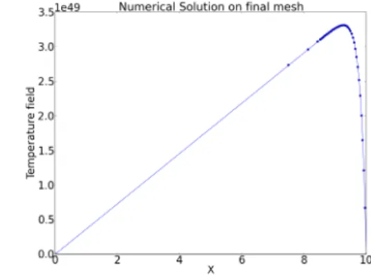
By taking q = 51, we can represent the analytical solution graphically as shown in figure 1. From figure 1, one can observe the sharp gradient of the field on the extreme right part of the bar.
3.2 Numerical Solution
We solved the problem numerically by taking q = 51. The solution can be rep-resented as shown in figure 2. From figure 2, one can observe that on the right hand side, where we have sharp gradient, we have greater number of elements to capture so-lution better. However, in the remaining part, algorithm puts fewer elements which are sufficient to represent the solution.
Figure 1: representation of analytical solution.
Figure 2: representation of numerical solution.
3.3 Analysis
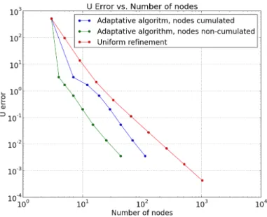
In order to assess the usefulness of this algorithm, we plot the error in calculated solution with respect to the number of nodes in log-log scale. We consider 3 cases. In the first case, we plot the error at each refinement iteration in adaptive mesh algorithm with respect to the cumulative number of nodes. We accumulate the number of nodes in this case because it will give us idea of not only the cost of calculating result on a particular mesh, but also it adds the cost of reaching to this particular mesh. In the second case, we plot error at each refinement iteration in adptative mesh algorithm with respect to the number of nodes in the mesh and in the third case, we plot error in uniform mesh refinement with respect to the number of nodes of each case. Figure 3 shows this plot for L2 norm of error in temperature field and figure 4 shows plot for error in energy norm error in the energy like potential.
Figure 4: energy norm error in energy like potential with respect to number of nodes.
4 Conclusions
In this work, we explained the variational approach for mesh refinement. We for-mulated the problem. Then we applied our hypothesis on a 1-D thermal problem.
In figures 3 and 4, we plotted L2 error norm in temperature field vs. number of nodes and energy error norm in energy vs. number of nodes respectively. In these graphs, we have also plotted the error vs. uniform refinements. The idea is that when mesh adaptation curve lies below the curve of uniform refinement, we have a better algorithm.(Less cost with equal or better precision.) Therefore, we plotted one curve with number of nodes accumulated and another with number of nodes. If we consider energy error as in figure 4, we see that variational algorithm is always better. However, if we consider error in temperature 3, the curve with non-accumulated nodes lies below the curve of refinement. But, the curve in which we accumulate the number of nodes, is first above the curve of uniform refinement, and as the algorithm progresses, it goes below. This behavior is logical because, the regions where variational adaptation curve is above the curve of uniform refinement, the mesh is too coarse.
Finally, we show that the variational mesh adaptation algorithm costs us less than a uniform mesh and still gives us better results.
The next part in the thesis is to apply this technique to the transient thermal problem and coupled thermo-mechanical problem using thermo-elasticity(Results of this part
will be shown in conference). Finally, we should extend this approach in 2D and 3D.
References
[1] J. MOSLER and M. ORTIZ. Variational h-adaptation in finite deformation elas-ticity and plaselas-ticity. International Journal of Numerical Methods in Engineering, 72:505–523, 2007.
[2] J. MOSLER and M. ORTIZ. An error-estimate-free and remapping-free variational mesh refinement and coarsening method for dissipative solids at finite strains.
In-ternational Journal of Numerical Methods in Engineering, 77:437–450, 2009. [3] M. ORTIZ and L. STAINIER. Variational formulation of viscoplastic constitutive
updates. Computational Methods for Applied Mechnical Engineering, 171:419– 444, 1999.