Série Scientifique
Scientific Series
95s-44
Estimating and Testing Exponential-Affine Term Structure
Models by Kalman Filter
Jin-Chuan Duan, Jean-Guy Simonato
Montréal octobre 1995
Ce document est publié dans l’intention de rendre accessibles les résultats préliminaires de la recherche effectuée au CIRANO, afin de susciter des échanges et des suggestions. Les idées et les opinions émises sont sous l’unique responsabilité des auteurs, et ne représentent pas nécessairement les positions du CIRANO ou de ses partenaires.
This paper presents preliminary research carried out at CIRANO and aims to encourage discussion and comment. The observations and viewpoints expressed are the sole responsibility of the authors. They do not necessarily represent positions of CIRANO or its partners.
CIRANO
Le CIRANO est une corporation privée à but non lucratif constituée en vertu de la Loi des compagnies du Québec. Le financement de son infrastructure et de ses activités de recherche provient des cotisations de ses organisations-membres, d’une subvention d’infrastructure du ministère de l’Industrie, du Commerce, de la Science et de la Technologie, de même que des subventions et mandats obtenus par ses équipes de recherche. La Série Scientifique est la réalisation d’une des missions que s’est données le CIRANO, soit de développer l’analyse scientifique des organisations et des comportements stratégiques.
CIRANO is a private non-profit organization incorporated under the Québec Companies Act. Its infrastructure and research activities are funded through fees paid by member organizations, an infrastructure grant from the Ministère de l’Industrie, du Commerce, de la Science et de la Technologie, and grants and research mandates obtained by its research teams. The Scientific Series fulfils one of the missions of CIRANO: to develop the scientific analysis of organizations and strategic behaviour.
Les organisations-partenaires / The Partner Organizations
•Ministère de l’Industrie, du Commerce, de la Science et de la Technologie. •École des Hautes Études Commerciales.
•École Polytechnique. •Université de Montréal. •Université Laval. •McGill University.
•Université du Québec à Montréal. •Bell Québec.
•La Caisse de dépôt et de placement du Québec. •Hydro-Québec.
•Fédération des caisses populaires de Montréal et de l’Ouest-du-Québec. •Téléglobe Canada.
•Société d’électrolyse et de chimie Alcan Ltée. •Avenor.
•Service de développement économique de la ville de Montréal. •Raymond, Chabot, Martin, Paré
The authors thank Eric Ghysels, Ked Hogan and the seminar participants at Chinese University of
%
Hong Kong, National Central University, National Taiwan University and National Tsing Hua University. Duan acknowledges the funding support by the Faculty of Management, McGill University.
McGill University and CIRANO
†
Université du Québec à Montréal and CIRANO
‡
Estimating and Testing Exponential-Affine Term
Structure Models by Kalman Filter
%%Jin-Chuan Duan , Jean-Guy Simonato
† ‡Résumé / Abstract
Cette recherche propose une approche unificatrice pour l'estimation des paramètres de modèles de structure de taux d'intérêt de la classe exponentielle-affine. Cette famille de modèles, caractérisée par Duffie et Kan (1993), contient entre autres les modèles de Vasicek (1977), Cox, Ingersoll et Ross (1985) et Chen et Scott (1992). La méthode proposée utilise un filtre de Kalman approximatif qui requiert la spécification de l'espérance et de la variance conditionnelle du système. La méthode utilise simultanément plusieurs séries de rendements et permet l'ajout d'erreurs de mesure pour chaque serie. Une étude de simulation indique que la méthode proposée est fiable pour des échantillons de taille modérée. Une étude empirique utilisant trois modèles différents de la classe exponentielle-affine est présentée.
This paper proposes a unified state-space formulation for parameter estimation of exponential-affine term structure models. This class of models, charaterized by Duffie and Kan (1993), contains models such as Vasicek (1977), Cox, Ingersoll and Ross (1985) and Chen and Scott (1992), among others. The proposed method uses an approximate linear Kalman filter which only requires specifying the conditional mean and variance of the system in an approximate sense. The method allows for measurement errors in the observed yields to maturitiy, and can simultaneously deal with many yields on bonds with different maturities. A Monte Carlo study indicates thet the proposed method is a reliable procedure for moderate sample sizes. An empirical analysis of three existing exponential-affine term structure models is carried out using monthly U.S. Treasury yield data with four different maturities. Our test results indicate a strong rejection of all three models.
Mots Clé : Structure à Terme, Filtre de Kalman, Exponentielle-affine, Modèle State-Space, Quasi-maximum de vraisemblance, Test du Multiplicateur de Lagrange Key Words : Term Structure, Kalman Filter, Exponential-Affine, State-Space Model, Quasi-Maximum Likelihood, Lagrange Multiplier Test
1. Introduction
The term structure of interest rates describes the relationship between the yield on a default{ free debt security and its maturity. Given the high correlation among bond yields of di®erent maturities, many theoretical models attempt to use a small number of factors to explain these joint movements. The typical macro{econometric approach is to specify a time{series model for the short{term interest rate and then employ the expectation hypothesis to derive a structural time series model for bond yields of di®erent maturities. Examples of this approach, such as Hamilton (1987) and Hall, Anderson and Granger (1992), are abundant in the literature.
A di®erent modelling approach, popular in the ¯nance literature and pioneered by Vasicek (1977) and Dothan (1978), starts out by assuming a di®usion process for the instantaneous spot interest rate. Arbitrage arguments are then used to facilitate the derivation of a bond pricing formula. According to these models, the bond price is a function of the unobserved instantaneous spot interest rate and the model's parameters. A more general approach is to assume a set of unobserved state variables and proceed to derive the bond price as a function of these state variables by arbitrage and/or equilibrium arguments. Cox, Ingersoll and Ross (1985) (hereafter CIR), Richard (1978), Longsta® and Schwartz (1992), and Chen and Scott (1992) are some examples. Recently, Du±e and Kan (1993) have provided a characterization for the class of exponential{a±ne term structure models, which contains most of the aforementioned term structure models as special cases. Among the existing term structure models, Vasicek (1977) and CIR (1985) have gained prominence in the literature of derivative contract pricing; for example, CIR (1985), Jamshidian (1989), Rabinovitch (1989), Hull and White (1990) and Duan, Moreau and Sealey (1995).
The empirical research focussing on some particular models of the exponential{a±ne family is extensive. The existent literature can be loosely classi¯ed into four categories. The ¯rst approach uses proxies for the unobserved factors; for example, Marsh and Rosenfeld (1983), Chan, et al. (1992) and Daves and Ehrhardt (1993). The second approach uses a
Examples of this approach are Brown and Dybvig (1986), Titman and Torous (1989), and De Munnik and Schotman (1994). The third category, such as Gibbons and Ramaswamy (1993), involves the derivation of conditional moment restrictions and the application of the generalized method of moments for estimation. The fourth category is the application of the transformed data maximum likelihood method proposed in Duan (1994). Particular cases of this approach are found in Pearson and Sun (1994) and Chen and Scott (1993a). The method proposed in this paper can be regarded as a generalization of the transformed data method. The transformed data method uses a term structure model to de¯ne a one-to-one data transformation from the unobserved state variables to the observed bond yields. This method breaks down when the number of yield series is greater than the number of state variables, unless one is willing to impose ad hoc restrictions on the structure of the measurement errors.
The purpose of this study is to develop a uni¯ed framework in which all exponential{ a±ne term structure models can be estimated with the simultaneous use of many bond yield series. We utilize a result of Du±e and Kan (1993) which establishes the su±cient and necessary conditions for the obtention of an exponential{a±ne term structure model. These conditions simply require the drift and variance functions of the underlying di®usion process to be a±ne in state variables. In this paper, we establish that the conditional mean and variance function of the state variables, over any discrete{time interval, must also be a±ne in state variables. This result for the discrete{time interval makes it possible to use the Kalman ¯lter and the prediction{error decomposition to obtain an approximate quasi{ maximum likelihood solution to the estimation problem for the entire class of exponential a±ne term structure models.
Special cases of our approach exist in the literature. To our knowledge, Pennacchi (1991) is the ¯rst study that uses a state-space formulation for estimating a term structure model of Gaussian nature. Chen and Scott (1993b) and Lund (1994) also propose the use of a Kalman ¯lter-based method to estimate term structure model. When our method is applied to a Gaussian model, if measurement errors are also normally distributed, our method becomes a maximum likelihood estimation.
The proposed method is implemented for the yields on the U.S. Treasury debt securities with maturities: 1, 3, 6, and 9 months. The empirical study is carried out using monthly data for the period from July, 1964 to February, 1992. Three term structure models of the exponential a±ne family { Vasicek (1977), CIR (1985), and Chen and Scott (1992) { are analyzed. For the Vasicek (1977) and CIR (1985) models, the parameter estimates in most cases are statistically signi¯cant. Using an approximate robust Lagrange multiplier test, we ¯nd that all three models are strongly rejected.
To examine the statistical properties of the proposed method, a Monte Carlo study is carried out. The simulation study suggests that the method is reasonably reliable even for a sample size as small as 150.
2. A State-Space formulation for the exponential{a±ne Term
Struc-ture Models
Vasicek (1977) and CIR (1985) bond pricing models have been widely used in the term struc-ture literastruc-ture. Both models involve specifying a stochastic process for the unobserved in-stantaneous spot interest rate. While Vasicek speci¯es a continuous time Ornstein-Uhlenbeck process, CIR use a mean-reverting square root process. Multi{factor generalizations of the CIR model have been proposed by Chen and Scott (1992) and Longsta® and Schwartz (1992). Recently Du±e and Kan (1993) have provided a characterization for the class of exponential{ a±ne term structure model which contains, amongst others, the aforementioned models as special cases.
The exponential{a±ne term structure model is a class of models in which the yields to maturity are a±ne functions in some abstract state variable vector Xt, which is assumed to
obey the following dynamic:
dXt= U(Xt; ª)dt + §(Xt; ª)dWt; (2.1)
where Wt is a n £ 1 vector of independent Wiener processes; ª denotes a p £ 1 vector
can be generically expressed as:
Dt(Xt; ª; ¿) = A(ª; ¿)e¡B(ª;¿)Xt; (2.2)
where Dt(Xt; ª; ¿) is the price at time t of a default{free discount bond with time to maturity
¿; A(ª; ¿) is a scalar function and B(ª; ¿) is a 1 £ n vector function. The instantaneous interest rate is, as usual, de¯ned as
rt(Xt; ª) = ¡ lim¿!0ln Dt(X¿t; ª; ¿): (2.3)
Du±e and Kan (1993) have shown that D(:) is generically exponential{a±ne, i.e. in the form of equation (2), if and only if U(:), §(:)§(:)0 and r
t(:) are a±ne in Xt. Moreover A(:) and
B(:) in equation (2) can be obtained as the solutions to some ordinary di®erential equations (see Appendix A).
Let Rt(Xt; ª; ¿) denote the time-t continuously compounded yield on a zero-coupon bond
of maturity ¿. The yield-to-maturity of this bond is given by:
Rt(Xt; ª; ¿) = ¡¿1ln(Dt(Xt; ª; ¿)): (2.4)
To deal with the estimation problem, it is reasonable to assume that the yields for di®erent maturities are observed with errors of unknown magnitudes. Using the bond pricing formula in (2), the yield to maturity can be written, after the addition of a measurement error, as:
Rt(Xt; ª; ¿) = ¡¿1ln(A(ª; ¿)) + 1¿B(ª; ¿)Xt+ ²t; (2.5)
where ²t is an error term with zero mean and standard deviation ¾². Note that ²t need not
be normally distributed.
Given that N bonds with di®erent maturities are observed, the N corresponding yields can be stacked to obtain the following representation:
2 6 6 6 6 4 Rt(Xt; ª; ¿1) Rt(Xt; ª; ¿2) ... Rt(Xt; ª; ¿N) 3 7 7 7 7 5= 2 6 6 6 6 4 ¡ ln(A(ª; ¿1))=¿1 ¡ ln(A(ª; ¿2))=¿2 ... ¡ ln(A(ª; ¿N))=¿N 3 7 7 7 7 5+ 2 6 6 6 6 4 (1=¿1)B(ª; ¿1) (1=¿2)B(ª; ¿2) ... (1=¿N)B(ª; ¿N) 3 7 7 7 7 5Xt+ 2 6 6 6 6 4 ²t;1 ²t;2 ... ²t;N 3 7 7 7 7 5: (2.6)
In terms of the state-space model, this equation is referred to as the measurement equation. To obtain the transition equation for the state-space model, we need to derive expressions for the conditional mean and variance of the unobserved state variables process over a discrete time interval of length h. De¯ne m(Xt; ª; h) ´ E(Xt+hjXt) and ©(Xt; ª; h) ´ Var(Xt+hjXt).
The transition equation over a discrete time interval, with length equal to h units of time, can be written as:
Xt+1= m(Xt; ª; h) + ©(Xt; ª; h)1=2´t+1 (2.7)
where ´t+1 is a n £ 1 vector of zero mean and unit variance error terms with ©(Xt; ª; h)1=2
denoting the Cholesky decomposition of ©(Xt; ª; h).
For a Gaussian state-space model, the Kalman ¯lter provides an optimal solution to pre-diction, updating and evaluating the likelihood function. The Kalman ¯lter recursion is a set of equations which allows an estimator to be updated once a new observation becomes available. The Kalman ¯lter ¯rst forms an optimal predictor of the unobserved state variable vector given its previously estimated value. This prediction is obtained using the distribu-tion of the unobserved state variables, condidistribu-tional on the previous estimated values. These estimates for the unobserved state variables are then updated using the information provided by the observed variables. Prediction errors, obtained as a by-product of the Kalman ¯lter, can then be used to evaluate the likelihood function.
When the state-space model is non-Gaussian, the Kalman ¯lter can still be applied to obtain approximate ¯rst and second moments of the model and the resulting ¯lter is quasi-optimal. The use of this quasi{optimal ¯lter yields an approximate quasi{likelihood function with which parameter estimation can be carried out.
Given that U(:) and §(:)§(:)0 are a±ne functions of X
t, m(Xt; ª; h) and ©(Xt; ª; h) must
be a±ne in Xt (see Appendix B). Let Ftbe the information set generated by the observations
up to and including time t. That is, Ft is a ¯ltration generated by fRs(Xs; ª; ¿1); ¢ ¢ ¢ ;
Rs(Xs; ª; ¿N); fors · tg. The conditional mean and variance are functions of the lagged
unobserved state variables. This implies that m(Xt; ª; h) and ©(Xt; ª; h) are not measurable
De¯ne Pt+1jt ´ Var(Xt+1jFt) and Pt´ Var(XtjFt). Because m(:) is a±ne in Xt we have:
m( ^Xt; ª; h) = a(ª; h) + b(ª; h) ^Xt; (2.8)
where a(:) and b(:) are n £ 1 and n £ n matrices and ^Xt ´ E(XtjFt). To implement
the quasi{optimal Kalman ¯lter, one must derive a relationship between Pt+1jt and Pt.
By the law of iterated expectations and recognizing that ©(Xt; ª; h) is a±ne in Xt and
Cov(Xt; ©(Xt; ª; h)1=2´t+1jFt) = 0 one can derive:
Pt+1jt= b(ª; h)Ptb(ª; h)0+ ©( ^Xt; ª; h): (2.9)
If it were possible to compute ^Xt, the conditional mean and variance of the system could
be correctly speci¯ed. Using the measurement and transition equations described in (6) and (7), the standard Kalman ¯lter recursion 1 could then be used to obtain a prediction-error
decomposition to evaluate the quasi-likelihood function. The estimates obtained with this quasi{likelihood function would, according to Bollerslev and Wooldridge (1992), are consis-tent and asymptotically normal. Unfortunately, the linear Kalman ¯lter cannot produce ^Xt;
rather it yields ¹Xt, that is the linear projection of Xt on the linear sub{space generated by
the observed yields. The conditional mean and variance computed with the estimate ¹Xt
should thus be di®erent from the true conditional mean and variance of the system. Never-theless, this approximation can be expected to work well because it is linearly optimal. This approximation is needed because of the non{Gaussian nature of the problem, which can be likened to linearizing a non{linear function in the typical Kalman ¯ltering applications.
Since ¹Xt is computable, we use it to approximate ^Xt which yields a quasi-likelihood
function in an approximate sense. This approximate quasi{likelihood function is used as if it were the correct quasi-likelihood function. Since the statistical properties of this procedure are theoretically unknown, Monte Carlo experiments are conducted in Section 4 to assess the quality of this procedure.
Let
LT(ª; R) = T
X
t=1lt(ª; Rt); (2.10)
where lt(ª; Rt) denotes the quasi-likelihood function at time t obtained from the
approxi-mate prediction-error decomposition with Rt = fRt(Xt; ª; ¿1); : : : ; Rt(Xt; ª; ¿N)g0 and R =
(R1; : : : ; RT). Following Bollerslev and Wooldridge (1992), it is reasonable to expect the
pa-rameter vector ^ªT maximizing LT(ª; R) to be approximately consistent and asymptotically
normal. This approximately consistent parameter should have the following approximate asymptotic distribution: p T ( ^ªT ¡ ª0) » N(0; ^FT¡1G^TF^T¡1); (2.11) where ^ FT = T1 T X t=1 ft(^ªT; Rt); (2.12) ^ GT = T1 T X t=1 @ ln lt( ^ªT; Rt) @ª 0 @ ln lt(^ªT; Rt) @ª ; (2.13) with ft( ^ª; Rt) = @¹ 0 t @ª¡1t @¹@ªt +12@ 0 t @ª[¡1t ¡1t ]@@ªt;
where ¹t and t are the conditional mean and variance functions obtained from the linear
Kalman ¯lter and @ ln lt(^ªT;Rt)
@ª , @¹@ªt and @@ªt are of dimension 1 £ p, N £ p and N2 £ p
respectively
The asymptotic covariance matrix of the quasi-maximum likelihood estimator, commonly referred to as the robust covariance matrix, is in general not equal to the inverse of Fisher's information matrix, ¡ limT !1F^T. For Gaussian exponential{a±ne term structure models,
the approximate quasi-likelihood function becomes the exact likelihood function if the mea-surement errors are normally distributed. This then implies that the asymptotic variance is (¡ limT !1F^T)¡1 or (limT !1G^T)¡1, a standard result.
To test the over{identi¯cation restrictions imposed by the theoretical model, an ap-proximate robust Lagrange multiplier test can be constructed. Denote the unconstrained
measurement equation to be: 2 6 6 6 6 4 Rt(Xt; ª; ¿1) Rt(Xt; ª; ¿2) ... Rt(Xt; ª; ¿N) 3 7 7 7 7 5= 2 6 6 6 6 4 ¡ ln(A(ª; ¿1))=¿1+ ®1 ¡ ln(A(ª; ¿2))=¿2+ ®2 ... ¡ ln(A(ª; ¿N))=¿N + ®N 3 7 7 7 7 5+ 2 6 6 6 6 4 (1=¿1)B(ª; ¿1) + ¯1 (1=¿2)B(ª; ¿2) + ¯2 ... (1=¿N)B(ª; ¿N) + ¯N 3 7 7 7 7 5Xt+ 2 6 6 6 6 4 ²t;1 ²t;2 ... ²t;N 3 7 7 7 7 5: (2.14) where ®1 to ®N are scalar parameters; ¯1 to ¯N are parameter vectors of dimension 1 £ n.
This speci¯cation for the unconstrained measurement equation is over{parameterized. First, the exponential{a±ne term structure model contains risk premium parameters that do not appear in the transition equation. Speci¯cally, risk premium parameters appear in functions A(:) and/or B(:) of the measurement equation. These risk premium parameters complicate the matter because the unconstrained model cannot be expressed solely in terms of the parameters ®i, ¯i and those in the transition equation. Second, since Xt is an
unob-served process, its location and scale parameters are indeterminate. This speci¯cation under the alternative hypothesis in equation (14) is thus under{identi¯ed.
To perform a Lagrange multiplier test of the null hypothesis, H0: ®i = 0; ¯i = 0 for all
i, one must deal with the over{parameterization problem by appropriately removing some parameters from the parameter space. More speci¯cally, n parameters must be removed to account for the risk premia, and 1
2n(n +1)+ n parameters removed for the alternative model
identi¯cation (see Harvey (1990), section 8.5.1). The decision about which parameters can be conveniently removed turns out to be model{speci¯c. We thus address this issue when the speci¯c bond pricing models are discussed in Section 3.
The approximate robust Lagrange multiplier test proceeds as follows. Denote by µ the parameter vector under the alternative, that is let µ0 = fª0; Á0g where Á is a parameter vector
of dimension N(n + 1) ¡1
2n(n + 1) ¡ 2n. The parameter vector ª is a subset of f®i; ¯ig after
removing an appropriate number of parameters. The null hypothesis can be stated as: H0 : Á = 0:
approximate robust LM test statistic as follows:
"LM = ^S1TF^T11C^11¡1F^T11^S1T0 ! Â2fN(n+1)¡1
2n(n+1)¡2ng; (2.15)
where ^F11
T is the partitioned inverse corresponding to Á; ^C = ^FT¡1G^TF^T¡1; and ^C11 is the
sub-matrix of ^C corresponding to Á; ^ST = @LT@µ(µ;R) and ^S1T is the subvector of ^ST corresponding
to Á.
3. Empirical results
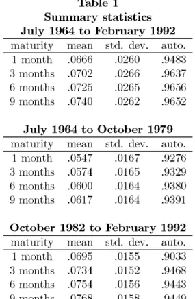
The data set used in this study consists of four monthly yield series for the U.S. Treasury debt securities with maturities: 1, 3, 6 and 9 months taken from the Fama{Bliss data ¯le. All interest rates are expressed on an annualized continuously compounded basis. These data series cover the period from July, 1964 to February, 1992, totalling 332 time series observations each. Table 1 reports summary statistics for these data series. Many empirical studies, for example, Hamilton (1988) and Spindt and Tarhan (1987), have found that the shift in the Federal Reserve monetary policy from October, 1979 to October, 1982, caused a structural break in the interest rate process. We thus report the results for the entire sample period as well as for two subperiods: July, 1964 to October, 1979 and October, 1982 to February, 1992.
The basic unit of time in this study is set equal to one year so that the maturities for all yields are stated in terms of the number of years and the parameter estimates can be interpreted as annualized values. Since the data frequency is monthly, the length of the discrete sampling interval, h, equals 1=12. The numerical optimization routine used in this study is the quadratic hill-climbing algorithm of Goldfeld, Quandt and Trotter (1966). The convergence criterion, based on the maximum absolute di®erence in both parameter and functional values between two successive iterations, is set to 0.0001. For each model examined below, the approximate Kalman ¯lter recursion is initialized with the stationary mean and variance of the unobserved state{variable(s).
3.1. The Gaussian case: Vasicek model
For the Vasicek (1977) model, the unobserved state variable is the instantaneous interest rate which has the following speci¯cation:
drt= ·(µ ¡ rt)dt + ¾dzt; (3.1)
where zt is a Wiener process; µ is the long{run average of the instantaneous spot interest
rate; · ¸ 0 is the mean{reverting intensity at which the process returns to its long{run mean; and ¾ > 0 is the volatility parameter of the process.
In terms of this model, the functional forms for A(:), B(:); a(:); b(:) and ©(:) are given by: A(ª; ¿) = e[°(B(ª;¿)¡¿)¡¾2B2(ª;¿)4· ]; (3.2) B(ª; ¿) = 1 · h 1 ¡ e¡·¿i; (3.3) ° = µ + ¾¸· ¡ 2·¾22; (3.4) a(ª; h) = µ(1 ¡ e¡·h); (3.5) b(ª; h) = e¡·h; (3.6) ©(Xt; ª; h) = ¾ 2 2·(1 ¡ e¡2·h); (3.7)
where ¸ is the risk premium parameter. In this model, ¸ > 0 implies a positive premium for bond prices.
We assume a diagonal covariance structure for the measurement errors. Its elements are denoted by ¾2 ²1, ¾ 2 ²3, ¾ 2 ²6, ¾ 2
²9. The second column of Tables 2A, B and C, present the
empirical results for the Vasicek model. Parameter estimates are reported along with their robust standard errors in parentheses. In Table 2A, the results for the entire sample period are reported. The long{run average interest rate, µ, the mean-reverting parameter · and ¾²6
are not signi¯cantly di®erent from zero at the usual signi¯cance level. All other parameters are signi¯cantly di®erent from zero. For the two sub{periods, reported in Tables 2B and 2C, all parameters are statistically signi¯cant except for · and ¾²6 in the ¯rst and second
When compared to the full sample estimates, the estimates for the pre{October, 1979 period as well as those for the post{October, 1982 period indicate a smaller instantaneous volatility, ¾. This result supports the ¯nding in the literature that the shift in the Federal Reserve monetary policy from October, 1979 to October, 1982 caused a structural break in the interest rate process.
The Lagrange multiplier test for the restrictions imposed by the Vasicek model on the coe±cients of the measurement equation is performed using the speci¯cation described at the end of Section 2. In order to make the factor model under the alternative hypothesis identi¯ed, ®1 and ¯1are conveniently removed from the unconstrained parameter space. For
the Vasicek model, only A(:) are functions of the risk premium parameter ¸. The parameter ®2 can be conveniently regarded as an extra parameter. It is thus also discarded from the
unconstrained model parameter space. As a result the degrees of freedom for this test on four yield series equals ¯ve. For the whole as well as sub-samples, the null hypothesis is strongly rejected as indicated at the bottom portion of Tables 2A, B and C.
3.2. The non-Gaussian case: Chen and Scott and CIR models
The Chen and Scott (1992) model allows for several independent state variables with the following dynamic:
dxi;t= ·i(µi¡ xi;t)dt + ¾ipxi;tdzi;t; (3.8)
for i = 1; :::; k and zi;t are independent Wiener processes.
In this section, the one and two{factor version of their model are analyzed. The one{ factor version of their model correspond to CIR (1985) model, where the unobserved factor is interpreted as the instantaneous interest rate.
For the two{factor model, the functional forms for A(:) and B(:) are given by:
A(ª; ¿) = A1(ª; ¿)A2(ª; ¿); (3.9)
where Ai(ª; ¿) and Bi(ª; ¿) for i = 1 and 2 have the following speci¯cation: Ai(ª; ¿) = " 2°ie[(·i+¸i+°i)¿]=2 (·i+ ¸i+ °i)(e°i¿ ¡ 1) + 2°i #2·iµi=¾2i ; (3.11) Bi(ª; ¿) = 2(e °i¿ ¡ 1) (·i+ ¸i+ °i)(e°i¿ ¡ 1) + 2°i; (3.12) with °i = q (·i + ¸i)2+ 2¾2i: (3.13)
The functional forms for a(:); b(:) and ©(:) are given by: a(ª; h) = ·µ1(1 ¡ e¡·1h) µ2(1 ¡ e¡·2h) ¸ ; (3.14) b(ª; h) = ·e¡·01h e¡·02h; ¸ ; (3.15) ©(Xt; ª; h) = ·© 1(x1;t; ª; h) 0 0 ©2(x2;t; ª; h) ¸ ; (3.16) with ©i(xt; ª; h) = xt¾ 2 i ·i(e ¡·ih¡ e¡2·ih) + µ i ¾ 2 i 2·i(1 ¡ e ¡·ih)2 (3.17)
where ¸1 and ¸2 are the risk premia parameters. In this model, ¸i < 0 implies a positive
premium in bond prices for factor i. The CIR (1985) model is a special case of this model, and is obtained by using the top left elements of the matrices de¯ned above.
The estimation results for the CIR (1985) model are reported in the third column of Tables 2A, B and C. These tables contain parameter estimates along with their corresponding robust standard errors in parentheses. Except for · in the second sub{sample and some measurement errors standard deviation, all estimates are signi¯cantly di®erent from zero at the 5% level in all samples. In all cases, the unobserved instantaneous interest rate is found to exhibit mean-reverting behavior, i.e., · > 0. The magnitude of the measurement errors are generally small but signi¯cantly di®erent from zero in many cases.
Comparing the estimates for the entire sample with the ones for the pre{October, 1979 and the post{October, 1982 periods reveals that a smaller volatility scale parameter, ¾, prevails for these two subperiods. These results are consistent with the previous ¯ndings
that the shift in the Federal Reserve monetary policy from October, 1979 to October, 1982 caused a structural break in the interest rate process. The mean-reverting property of the interest rate process again prevails for these two subperiods.
The Lagrange multiplier test of the restrictions imposed by the CIR model on the coef-¯cients of the measurement equation is performed using the speci¯cation described at the end of Section 2. For the CIR model, both A(:) and B(:) are functions of the risk premium parameter ¸. As with the Vasicek model, we remove ®1, ®2 and ¯1 from the unconstrained
parameter space to make the model identi¯ed under the alternative speci¯cation. As a re-sult, the degrees of freedom for this test equals ¯ve. The null hypothesis is strongly rejected in the three samples as shown by the P-values of the Chi-square tests.
The estimation results for the Chen and Scott (1992) model are reported in the fourth column of Tables 2A, B and C. These tables contain parameter estimates along with their corresponding robust standard errors in parentheses. For the entire sample period and the ¯rst sub{sample, all parameters are signi¯cantly di®erent from zero except for µ2, ·2 and ¸2.
For the second sub-samples only µ2 and ·2 are not signi¯cantly di®erent from zero.
The most striking feature of these estimates are the small values for µ2 and ·2. With
these values, ¾2
2 > 2·2µ2 and the second factor can reach zero with a positive probability
(see CIR (1985)). A small value for ·2 also suggest that the second factor is close to being
non stationary. The resulting test statistics might therefore di®er from the approximate asymptotic normal distribution and should be interpreted with care.
Comparing the estimates for the entire sample with the ones for the pre{October, 1979 and post{October, 1982 periods still points to a structural instability even when the two{ factor model is used. This result is once again consistent with the previous ¯ndings that the shift in the Federal Reserve monetary policy from October, 1979 to October, 1982 caused a structural break in the interest rate process.
Chen and Scott (1993b) report the estimation results for the Chen and Scott (1992) two-factor model. Their estimates are consistent with our ¯ndings. More speci¯cally, the estimates for the long{run mean and mean reversion parameters of the second factor are
In the Chen and Scott (1992) model, both A(:) and B(:) are functions of the risk premium parameters. To perform the robust Lagrange multiplier test described at the end of Section 2, ¯N, which is a 1 £ n vector, can be conveniently removed from the parameter space
to account for the risk premium parameters. To ensure that the factor model under the alternative speci¯cation is identi¯ed, ®1, ®2, ¯1 and the second entry of ¯2 are removed from
the unconstraint parameter space. The resulting degrees of freedom for this Chi{square test also equals ¯ve. In all samples the null hypothesis is strongly rejected as indicated by the P-values of the Chi-square tests.
4. A Monte Carlo analysis
To assess the statistical properties of the proposed method, we conduct Monte Carlo exper-iments for the sample size of 150, 350 time-series observations with the simultaneous use of 1-, 3-, 6- and 9-month maturities. These sample sizes are chosen because they roughly correspond to the sub and whole sample size of the data sets analyzed in the preceding section.
To perform Monte Carlo experiments, the unobserved state variables of a given model must ¯rst be simulated. For the Vasicek (1977) model, the state variable follows an Ornstein{ Uhlenbeck process which can be obtained using the exact conditional distribution. More formally, denote r¤
t to be the simulated value of the process at time t. Using the transition
density of this process, r¤
t is obtained by:
r¤
t ¡ rt¡h¤ = µ + (r¤t¡h¡ µ) e¡·h +
q
Á²t;
where ²t is N(0; 1) with r0¤ = µ and Á = ¾ 2
2·(1 ¡ e¡2·h) and h set to 1=12.
For the square{root process in CIR (1985), the exact conditional distribution is also used to obtain the simulated values. Let xt denote the value of an unobserved state variable
following a square{root process. The conditional distribution function for xt is the non{
central chi{square, Â2[ 2cx
t; 2d + 2; 2w], with 2d + 2 degrees of freedom and parameter of
non{centrality 2w where
d = 2·µ¾2 ¡ 1; w = cxt¡he¡·h:
As discussed in Johnson and Kotz (1970), the non{central Chi-square distribution can be expressed as a mixture of central Chi-squares with degrees of freedom proportional to random variates from a Poisson distribution. This property is used to simulate the process. More precisely, x¤
t, the simulated value of the process at time t, is obtained by the following steps:
1. Simulate the degrees of freedom of the central chi{square using df = 2d + 2 + 2j;
where j is a Poisson random variate 2 with mean w = cx¤
t¡he¡·h. The time interval h
is set to 1=12 and x¤ 0 = µ.
2. Let g denote the random variate drawn from the central chi{square with df degrees of freedom. This random variate is obtained from a gamma (df
2; 2) random variate 3
where df
2 is the shape parameter and 2 is the scale parameter.
3. Compute x¤ t = 2cg.
Using the simulated time series for either the Ornstein{Uhlenbeck or the square-root process, equation (5) is then used to compute the simulated yields with independent normally distributed measurement errors. The Monte Carlo simulation results for discretely sampled time-series are reported for the Gaussian case (Vasicek (1977)) and the non{Gaussian case (CIR (1985)). The results are obtained using 500 repetitions.
Rows one, two, three and four of Tables 3 and 4 report the true parameter values, the medians, the means and the standard deviations of the parameter estimates. The remaining four rows report the probability that the true parameter lies in the ®% con¯dence interval. This probability is referred to as the ®% coverage rate. For example, to obtain 95% cov-erage rate, Probfjªi¡ ^ªiTj < 1:96 s:e:( ^ªiT)g is to be computed, where ªi denotes the ith
parameter of the model and s:e:(^ªiT) represents the estimated standard error for the ith
parameter estimator. The bottom row of each panel reports the 95% coverage rate for the over{identi¯cation test statistic. This value indicates whether the test is biased or not.
The Monte Carlo simulation results for the Gaussian case (Vasicek (1977) model) are pre-sented in Table 3A. The true parameter values are taken from the estimates, after rounding, in the empirical section. The estimated values are exceedingly close to their correspond-ing true values for all parameters except µ and ·. The magnitude of the bias for these two parameters is small as a percentage of their corresponding true values. The coverage rates of the parameters indicate some departure from the asymptotic distribution, especially when a smaller sample size is used. A possible explanation for this departure is the small value given to ·. As · approaches zero, the unobserved factor and the yield series become non{stationary.
To investigate further, additional Monte Carlo experiments with 350 observations and di®erent parameter values are are reported in the third panel of Table 3B. The top panel of this table reports the results for the case of a larger value for ·, the mean{reverting parameter. When · = :5, the biases nearly vanish, and the asymptotic distribution becomes a better approximation to the small sample distribution. The bottom panel of this table reports the results for the case of a smaller mean{reverting parameter value. When its value is set to 0.01, the coverage rates become similar to those reported in the second panel of Table 3A. This result suggests that the magnitude of the mean reversion parameter plays an important role in determining the quality of the estimator when using a ¯nite sample size. This result is not surprising. The mean{reverting parameter · is a transformation of the ¯rst order autoregressive parameter. It is well known in the time{series literature that the standard asymptotic properties of the estimators do not hold in the presence of a unit root. The 95% coverage rate of the Lagrange multiplier test indicates a slight departure from the asymptotic distribution for all Monte Carlo experiments in Table 3. The test appears more conservative, meaning that the null hypothesis is rejected slightly more than 5% of the time.
in Table 4A. The true parameter values are taken from the estimates, after rounding, in the preceding empirical section. The estimates are close to their corresponding true values for all parameters. As with the Vasicek (1977) model, µ and · are slightly biased. However, the magnitude of the bias is small as a percentage of the true parameter value. Overall the coverage rates of the parameters indicate that the asymptotic distribution to the quasi{ maximum likelihood estimator is a good approximation of the small sample distribution. In order to assess the impact of a nearly integrated factor, additional Monte{Carlo experiments with 350 observations and di®erent parameter values are reported in Table 4B. The top portion of this table reports the results for a larger value of ·. As in the Gaussian case with · = :5, the biases nearly vanish, and the approximate asymptotic distribution becomes a better approximation to the small sample distribution. The bottom panel of this table reports the results for the same parameter values with the exception of ·, which is now set to 0.01, a value closer to zero. With these parameter values, the estimates for µ and · are biased and their coverage rates are poorly approximated by the asymptotic distribution.
Again, as with the Gaussian case, the 95% coverage rate of the Lagrange multiplier test also indicates some departure from the asymptotic distribution in all Monte Carlo experi-ments in Table 4A. The test is typically more conservative, meaning that the null hypothesis is rejected more than 5% of the time. Interestingly, the case with a smaller value for · in the bottom panel of Table 4B actually yields a better result for the Lagrange multiplier test.
Overall, these results suggest that the approximate quasi{maximum likelihood estimator, the CIR case, and the maximum likelihood estimator, the Vasicek case, tend to behave in a similar fashion. Both estimators are sensitive to a nearly integrated factor, and both estimators tend to slightly over{reject the null hypothesis in the Lagrange multiplier test. By and large, the ¯nite sample properties of the approximate quasi{maximum likelihood estimator are reasonably described by their asymptotic equivalents.
5. Conclusion
In this article, a uni¯ed state-space formulation is developed for estimating term structure models of the exponential{a±ne family. The method allows for measurement errors in the ob-served yields to maturity, and is therefore useful for simultaneous estimation using yields on many bonds with di®erent maturities. The quasi-optimal Kalman ¯ltering approach can be useful for implementing derivative asset pricing models that are based on these exponential{ a±ne term structure models. This estimation method is able to produce parameter estimates as well as a linearly ¯ltered estimate of the unobserved state variables. Since the parameter estimates and the ¯ltered state variables can be obtained by using a set of yields that cover a desirable maturity spectrum, its application to derivative asset pricing is likely to be less in°uenced by the measurement error in any given yield series.
A Monte Carlo study indicates that the proposed method is an adequate procedure. The ¯nite sample properties of the approximate quasi{maximum likelihood estimator are reasonably approximated by the asymptotic distribution presented in this paper.
Three special cases of the exponential{a±ne family are used to examine the estimation method. The empirical results are, in some instances, supportive of the properties typical of the exponential{a±ne term structure models; for example, the mean-reverting property of the interest rate process. This, however, does not suggest that the three exponential{ a±ne term structure models analyzed in this paper are good descriptions of the bond yield behaviour. In fact the results from using four di®erent maturities cast doubts as to whether these models can be applied to yields covering a large maturity spectrum. Using a robust Lagrange multiplier test, the three exponential a±ne models are strongly rejected. These results suggest that future research is needed in order to ¯nd a better speci¯cation within or beyond the exponential{a±ne family.
References
Bollerslev, T.P., and J.M. Wooldridge, 1992, Quasi-Maximum Likelihood Estimation and Inference in Dynamic Models with Time-Varying Covariances, Econometric Reviews 11, 143{172.
Brown, S.J. and P.H. Dybvig, 1986, The Empirical Implications of the Cox, Ingersoll, Ross Theory of the Term Structure of Interest Rates, Journal of Finance 41, 617{630.
Chan, K.C., G.A. Karolyi, F.A. Longsta®, and A.B. Sanders, 1992, Comparison of Models of the Short-Term Interest Rate, Journal of Finance 47, 1209{1227.
Chen, R., and L. Scott, 1992, Pricing Interest Rate Options in a Two{Factor Cox{Ingersoll{ Ross Model of the Term Structure, Review of Financial Studies 5, 613{636.
Chen, R., and L. Scott, 1993a, Maximum Likelihood Estimation for a Multi-Factor Equilib-rium Model of the Term Structure of Interest Rates, Journal of Fixed Income 4, 14{31. Chen, R., and L. Scott, 1993b, Multi-Factor Cox- Ingersoll-Ross Models of the Term
Struc-ture: Estimates and Tests from a State-Space Model Using a Kalman Filter, Unpublished manuscript, University of Georgia.
Cox, J., J. Ingersoll and S. Ross, 1985, A Theory of the Term Structure of Interest Rates, Econometrica 53, 385{407.
Daves, P. and M. Ehrhardt, 1993, Joint Cross-Section/Time-Series Maximum Likelihood Estimation for the Parameters of the Cox-Ingersoll-Ross Bond Pricing Model, Financial Review 28, 203{237.
De Munnik, J. and P. Schotman, 1994, Cross Sectional Versus Time Series Estimation of Term Structure Models: Empirical Results for the Dutch Bond Market, Journal of Bank-ing and Finance 18, 997{1025.
Devroye, L., 1981, The Computer Generation of Poisson Random Variables, Computing 26, 197-207.
Devroye, L., 1986, Non-Uniform Random Variate Generation, Springer-Verlag, New-York. Domowitz, I. and H. White, 1982, Misspeci¯ed Models with Dependent Observations,
Jour-nal of Econometrics 20, 35{58.
Dothan, U.L., 1978, On the Term Structure of Interest Rates, Journal of Financial Economics 6, 59{69.
Duan, J.-C., A. Moreau and C.W. Sealey, 1995, Deposit Insurance and Bank Interest Rate Risk: Pricing and Regulatory Implications, Journal of Banking and Finance, forthcoming. Du±e, D. and R. Kan, 1993, A Yield{Factor Model of Interest Rates, Unpublished Manuscript,
Graduate School of Business, Stanford University.
Gibbons, M. and K. Ramaswamy, 1993, A Test of the Cox, Ingersoll, and Ross Model of the Term Structure, Review of Financial Studies 6, 619{658.
Goldfeld, S.M., R.E. Quandt and H.F. Trotter, 1966, Maximization by Quadratic Hill-Climbing, Econometrica 34, 541{551.
Hall, A.D., H.M. Anderson and C.W.J. Granger 1992, A Cointegration Analysis of Treasury Bill Yields, Review of Economics and Statistics 74, 116{126.
Hamilton, J.D., 1987, Rational{Expectations Econometric Analysis of Changes in Regime, An Investigation of the Term Structure of Interest Rates, Journal of Economic Dynamics and Control 12, 385{423.
Harvey, A.C., 1990, Forecasting, Structural Time Series Models and the Kalman Filter, Cambridge University press, Cambridge.
Hull, J. and A. White, 1990, Pricing Interest-Rate Derivative Securities, Review of Financial Studies 3, 573{592.
Johnson, N.L. and S. Kotz, 1970, Distributions in Statistics: Continuous Univariate Distri-butions { 2. Houghton Mi±n Company, Boston.
Longsta®, F.A., and E.S. Schwartz, 1992, Interest Rate Volatility and the Term Structure: A Two-Factor General Equilibrium Model, Journal of Finance 47, 1259{1282.
Lund, J., 1994, Econometric Analysis of Continuous{Time Arbitrage{Free Models of the Term Structure of Interest Rates, Unpublished manuscript, Aarhus School of Business. Marsh, T.A. and E.R. Rosenfeld, 1983, Stochastic Processes for Interest Rates and
Equilib-rium Bond Prices, Journal of Finance 38, 635{646.
Pennacchi, G., 1991, Identifying the Dynamics of Real Interest Rates and In°ation: Evidence Using Survey Data, Review of Financial Studies 4, 53{86.
Pearson, N.D. and T.S. Sun, 1994, Exploiting the Conditional Density in Estimating the Term Structure: An Application to the Cox, Ingersoll, and Ross Model, Journal of Finance 49, 1279{1304.
Financial Economics 6, 33{57.
Rabinovitch, R., 1989, Pricing Stock and Bond Options When the Default{Free Rate is Stochastic, Journal of Financial and Quantitative Analysis 24, 447{457.
Spindt, P.A. and V. Tarhan, (1987), The Federal Reserve's New Operating Procedures, A Post Mortem, Journal of Monetary Economics 19, 107{123.
Titman, S. and W. Torous, 1989, Valuing Commercial Mortgages: An Empirical Investiga-tion of the Contingent-Claims Approach to Pricing Risky Debt, Journal of Finance 44, 345{374.
Vasicek, O., 1977, An Equilibrium Characterization of the Term Structure, Journal of Fi-nancial Economics 5, 177{188.
White, H., 1982, Maximum Likelihood estimation of Misspeci¯ed Models, Econometrica 50, 1{25.
Appendix A
Di®erential equations for A(:) and B(:) functions.As shown in Du±e and Kan (1993), the solutions for the A(:) and B(:) functions can be found by solving the following di®erential equations:
¡@B(ª; ¿)
@t + B(B(ª; ¿)) = 0; B(ª; 0) = 0; ¡@A(ª; ¿)@t + A(B(ª; ¿)) = 0; A(ª; 0) = 0; with ¡@Bi(ª;¿)
@t + Bi(B(ª; ¿)) denoting the coe±cients of Xi;t and ¡@A(ª;¿)@t + B(B(ª; ¿))
denoting the term not involving Xt in the following equation:
rt(Xt; ª) = ¡@A(ª; ¿)@t ¡ @B(ª; ¿)@t Xt+ B(ª; ¿)U(Xt; ª) +12Xn i=1 n X j=1 Bi(ª; ¿)Bj(ª; ¿)§i(Xt; ª)§j(Xt; ª)0;
where §i(:) is the ith line of matrix §(:).
Appendix B
Theorem: Assume that the n £ 1 vector Xt obeys the following dynamic:
dXt= U(Xt; ª)dt + §(Xt; ª)dWt:
Suppose that U(Xt; ª) and §(Xt; ª)§(Xt; ª)0 are a±ne functions of Xt so that U(Xt; ª)
can be written as G + KXt with G and K being matrices of dimension n £ 1 and n £ n. The
mean and variance of Xt+h, conditional on Xt, are a±ne functions of Xt if K is diagonable.
Remark: A matrix is diagonable if all of its eigenvalues are distinct. The assumption of diagonability does not involve an appreciable loss of generality. Since the eigenvalues of a
matrix are continuous functions of its elements, if the matrix K has multiple eigenvalues, a slight alteration to any element produces a neighbouring system with distinct roots that, for all practical purposes, is the same as the original system. Therefore the statement of the theorem is a generic result.
Proof:
For notational convenience, let §(Xt; ª) = §t. The integral representation for Xt+h can
be written as: Xt+h = Xt+ Z t+h t [G + KXs]ds + Z t+h t §sdWs:
Denote the eigenvalue decomposition of K, usually a non{symmetric matrix, by QkQ¡1
where Q¡1Q = I and k a square diagonal matrix. Premultiplying the above equation by
Q¡1 yields: Yt+h = Yt+ Z t+h t [g + kYs]ds + Z t+h t ¾sdWs;
where Yt = Q¡1Xt, g = Q¡1G, and ¾t = Q¡1§t. Taking conditional expectation gives rise
to:
E(Yt+hjYt) = Yt+
Z t+h
t [g + kE(YsjYt)]ds:
The solution to this integral equation is:
E(Yt+hjYt) = ekhYt¡ (ekh¡ I)k¡1g:
The solution for E(Xt+hjXt) can be recovered from the above solution which is an a±ne
function of Xt.
The conditional variance of Yt can be computed using:
by stacking the individual elements of the upper triangle of Yt+hYt+h0 . That is let: ft = 2 6 6 6 6 6 6 6 6 6 6 6 6 6 6 4 Y1;tY1;t Y1;tY2;t ... Y1;tYn;t Y2;tY2;t Y2;tY3;t ... Yn;tYn;t 3 7 7 7 7 7 7 7 7 7 7 7 7 7 7 5 = 2 6 6 6 6 6 6 6 6 6 6 6 6 6 6 4 f1;1 t ft1;2 ... ft1;n ft2;2 f2;3 t ... ftn;n 3 7 7 7 7 7 7 7 7 7 7 7 7 7 7 5 :
Using Ito's lemma on ft yields:
ft+h= ft+ Z t+h t " @fs @Ysus+ Dsds # +Z t+h t ¾s @fs @YsdWs;
where ut= g + kYt with k being the diagonal matrix de¯ned earlier. Moreover,
@ft @Yt = 2 6 6 6 4 @ft1;1 @Y1;t @ft1;1 @Y2;t : : : @ft1;1 @Yn;t ... ... ... ... @ftn;n @Y1;t @ftn;n @Y2;t : : : @ftn;n @Yn;t 3 7 7 7 5; Dt= 12 2 6 6 6 4 tr(¾t¾t0 @ 2f1;1 t @Yt@Yt0) ... tr(¾t¾t0@ 2fn;n t @Yt@Yt0) 3 7 7 7 5; and @2fi;j t @Yt@Yt0 = 2 6 6 6 4 @2fi;j t @Y1;t@Y1;t : : : @2fi;j t @Y1;t@Yn;t ... ... ... @2fi;j t @Yn;t@Y1;t : : : @2fi;j t @Yn;t@Yn;t 3 7 7 7 5:
Since ut is a±ne in Yt, we can write:
@ft
@Ytut= pYt+ qft;
[(n+1)n 2 ] given by: q = 2 6 6 6 6 4 k1;1+ k1;1 0 : : : 0 0 k1;1+ k2;2 : : : 0 ... ... ... ... 0 0 : : : kn;n+ kn;n 3 7 7 7 7 5;
where ki;j is element i; j of matrix k. Since ¾t¾t0 is a±ne in Yt, it follows that:
Dt= w + vYt;
where w and v are matrices of dimension [(n+1)n2 ] £ 1 and [(n+1)n2 ] £ n, respectively. The stochastic integral equation can thus be rewritten as:
ft+h = ft+ Z t+h t [pYs+ qfs+ w + vYs]ds + Z t+h t ¾s @fs @YsdWs:
Taking conditional expectation yields: E(ft+hjYt) = ft+
Z t+h
t [zs+ qE(fsjYt)]ds;
where zs= w + (p + v)E(YsjYt). Clearly, zs is a function of s and is an a±ne function of Yt.
The solution to this integral equation is
E(ft+hjYt) = eqhft+
Z t+h
t e
q(t+h¡s)z sds:
As this solution shows, the only non{a±ne element, in terms of Yt, for E(Yt+hYt+h0 jYt) is
given by
eqhf t:
Straightforward computations for E(Yt+hjYt)E(Yt+hjYt)0, shows that the only non{a±ne
ele-ment is given by
ekhY
tYt0ekh:
The upper triangular elements of this matrix, when properly staked up, are precisely the elements of eqhf
Table 1 Summary statistics July 1964 to February 1992 maturity mean std. dev. auto.
1 month .0666 .0260 .9483
3 months .0702 .0266 .9637
6 months .0725 .0265 .9656
9 months .0740 .0262 .9652
July 1964 to October 1979 maturity mean std. dev. auto.
1 month .0547 .0167 .9276
3 months .0574 .0165 .9329
6 months .0600 .0164 .9380
9 months .0617 .0164 .9391
October 1982 to February 1992 maturity mean std. dev. auto.
1 month .0695 .0155 .9033
3 months .0734 .0152 .9468
6 months .0754 .0156 .9443
Table 2A
Estimation results for the Vasicek (1977), CIR (1985) and Chen and Scott (1992) models
with monthly observations on 1, 3, 6 and 9 months yield series
July 1964 to February 1992
Parameters Model
Vasicek CIR Chen and Scott
µ1 0.0486 0.0633 0.0285 (0.0350) (0.0111) (0.0015) ·1 0.0561 0.3189 5.5699 (0.0351) (0.0665) (0.6103) ¾1 0.0225 0.0750 0.1481 (0.0022) (0.0052) (0.0183) ¸1 0.8039 -0.2715 -1.5747 (0.0979) (0.0572) (0.2232) µ2 { { 1.2e-7 { { (2.4e-6) ·2 { { 0.0006 { { (0.1146) ¾2 { { 0.1052 { { (0.0074) ¸2 { { -0.0449 { { (0.1307) ¾²1 0.0058 0.0058 0.0041 (0.0004) (0.0004) (0.0003) ¾²3 0.0025 0.0025 0.0013 (0.0002) (0.0002) (0.0001) ¾²6 4.23e-8 3.8e-9 0.0004 (1.0662) (15.010) (0.0002) ¾²9 0.0018 0.0018 0.0013 (0.0001) (0.0001) (0.0001) Chi-square 115.21 146.98 48.756 P-value 0.0000 0.0000 0.0000 df 5 5 5
Table 2B
Estimation results for the Vasicek (1977), CIR (1985) and Chen and Scott (1992) models
with monthly observations on 1, 3, 6 and 9 months yield series
July 1964 to October 1979
Parameters Model
Vasicek CIR Chen and Scott
µ1 0.0626 0.0602 0.0265 (0.0316) (0.0106) (0.0024) ·1 0.0591 0.3628 5.3813 (0.0428) (0.0737) (0.6536) ¾1 0.0153 0.0637 0.1068 (0.0013) (0.0045) (0.0160) ¸1 1.2520 -0.3205 -1.4781 (0.1449) (0.0650) (0.2339) µ2 { { 1.3e-7 { { (0.0002) ·2 { { 0.0001 { { (0.1408) ¾2 { { 0.0926 { { (0.0074) ¸2 { { -0.1567 { { (0.1556) ¾²1 0.0034 0.0034 0.0019 (0.0002) (0.0002) (0.0002) ¾²3 0.0020 0.0020 0.0012 (0.0002) (0.0002) (0.0002) ¾²6 0.0003 0.0002 0.0006 (0.0004) (0.0004) (0.0001) ¾²9 0.0018 0.0018 0.0014 (0.0001) (0.0001) (0.0001) Chi-square 65.123 91.616 25.433 P-value 0.0000 0.0000 0.0001 df 5 5 5
Table 2C
Estimation results for the Vasicek (1977), CIR (1985) and Chen and Scott (1992) models
with monthly observations on 1, 3, 6 and 9 months yield series
October 1983 to February 1992
Parameters Model
Vasicek CIR Chen and Scott
µ1 0.0609 0.0606 0.0352 (0.0302) (0.0181) (0.0015) ·1 0.0094 0.0791 5.0808 (0.0096) (0.0637) (0.8336) ¾1 0.0131 0.0467 0.1152 (0.0010) (0.0036) (0.0196) ¸1 1.0812 -0.1998 -0.8669 (0.0955) (0.0243) (0.2226) µ2 { { 1.6e-5 { { (0.0015) ·2 { { 2.2e-5 { { (0.0020) ¾2 { { 0.0764 { { (0.0081) ¸2 { { -0.1338 { { (0.0463) ¾²1 0.0059 0.0059 0.0042 (0.0007) (0.0007) (0.0006) ¾²3 0.0021 0.0021 0.0006 (0.0003) (0.0003) (0.0002) ¾²6 7.3e-8 2.2e-8 0.0005 (0.7372) (5.1004) (0.0001) ¾²9 0.0013 0.0013 0.0005 (0.0001) (0.0002) (0.0001) Chi-square 48.020 98.839 41.666 P-value 0.0000 0.0000 0.0000 df 5 5 5
Table 3A
Monte-Carlo experiment results for the maximum likelihood parameter estimator of the Vasicek model for 1, 3, 6 and 9-month yields
(500 replications) T=150 observations µ · ¾ ¸ ¾²1 ¾²3 ¾²6 ¾²9 true value 0.0500 0.0600 0.0200 0.8000 0.0010 0.0010 0.0010 0.0010 median 0.0524 0.0601 0.0199 0.8003 0.0010 0.0010 0.0010 0.0010 mean 0.0521 0.0625 0.0199 0.8022 0.0010 0.0010 0.0010 0.0010 std. dev. 0.0254 0.0173 0.0012 0.0920 0.0001 0.0001 0.0001 0.0001 cov. rate 25% cov. rate 0.2740 0.2040 0.2340 0.2540 0.2360 0.2220 0.2420 0.2200 50% cov. rate 0.4840 0.4220 0.4560 0.5460 0.4800 0.4580 0.4820 0.4280 75% cov. rate 0.9320 0.6600 0.7000 0.8280 0.7520 0.7200 0.7420 0.7160 95% cov. rate 1.0000 0.9080 0.9340 0.9860 0.9620 0.9420 0.9320 0.9260
95% cov. rate for Lagrange multiplier test: 0.9380
T=350 observations T=350 observations µ · ¾ ¸ ¾²1 ¾²3 ¾²6 ¾²9 true value 0.0500 0.0600 0.0200 0.8000 0.0010 0.0010 0.0010 0.0010 median 0.0510 0.0612 0.0200 0.7981 0.0010 0.0010 0.0010 0.0010 mean 0.0511 0.0611 0.0200 0.7989 0.0010 0.0010 0.0010 0.0010 std. dev. 0.0295 0.0078 0.0008 0.0942 0.0001 0.0001 0.0000 0.0001 cov. rate 25% cov. rate 0.2220 0.2260 0.2720 0.2300 0.2240 0.2380 0.2500 0.2000 50% cov. rate 0.4760 0.4120 0.4860 0.4660 0.4340 0.4540 0.4860 0.4200 75% cov. rate 0.8120 0.7180 0.7280 0.8040 0.6880 0.7220 0.7540 0.7020 95% cov. rate 1.0000 0.9260 0.9380 0.9980 0.9260 0.9420 0.9520 0.9420
Table 3B
Monte-Carlo experiment results for the maximum likelihood parameter estimator of the Vasicek model for 1, 3, 6 and 9-month yields
(500 replications) T=350 observations µ · ¾ ¸ ¾²1 ¾²3 ¾²6 ¾²9 true value 0.1000 0.5000 0.0500 1.0000 0.0010 0.0010 0.0010 0.0010 median 0.1006 0.5000 0.0499 0.9877 0.0010 0.0010 0.0010 0.0010 mean 0.1006 0.5002 0.0499 0.9972 0.0010 0.0010 0.0010 0.0010 std. dev. 0.0167 0.0058 0.0019 0.1713 0.0001 0.0001 0.0000 0.0001 cov. rate 25% cov. rate 0.2220 0.2400 0.2720 0.2260 0.2240 0.2380 0.2460 0.2120 50% cov. rate 0.4460 0.4680 0.5100 0.4360 0.4360 0.4540 0.4740 0.4180 75% cov. rate 0.7060 0.7500 0.7200 0.7200 0.6860 0.7180 0.7560 0.7040 95% cov. rate 0.9440 0.9360 0.9500 0.9440 0.9340 0.9360 0.9480 0.9360
95% cov. rate for Lagrange multiplier test: 0.9320
T=350 observations T=350 observations µ · ¾ ¸ ¾²1 ¾²3 ¾²6 ¾²9 true value 0.1000 0.0100 0.0500 1.0000 0.0010 0.0010 0.0010 0.0010 median 0.1003 0.0105 0.0499 1.0007 0.0010 0.0010 0.0010 0.0010 mean 0.1021 0.0105 0.0500 1.0019 0.0010 0.0010 0.0010 0.0010 std. dev. 0.0734 0.0026 0.0019 0.0397 0.0001 0.0001 0.0000 0.0001 cov. rate 25% cov. rate 0.6120 0.2060 0.2760 0.2980 0.2180 0.2300 0.2560 0.2180 50% cov. rate 0.8100 0.3960 0.5160 0.5500 0.4420 0.4540 0.4820 0.4240 75% cov. rate 1.0000 0.6600 0.7160 0.7960 0.6860 0.7160 0.7540 0.7020 95% cov. rate 1.0000 0.8740 0.9480 0.9680 0.9320 0.9400 0.9540 0.9400
Table 4A
Monte-Carlo experiment results for the approximate quasi{maximum likelihood parameter estimator of
the CIR model for 1, 3, 6 and 9-month yields (500 replications) T=150 observations µ · ¾ ¸ ¾²1 ¾²3 ¾²6 ¾²9 true value 0.0600 0.3000 0.0750 -0.3000 0.0010 0.0010 0.0010 0.0010 median 0.0560 0.3215 0.0748 -0.3224 0.0010 0.0010 0.0010 0.0010 mean 0.0580 0.3235 0.0748 -0.3207 0.0010 0.0010 0.0010 0.0010 std. dev. 0.0107 0.0595 0.0045 0.0548 0.0001 0.0001 0.0001 0.0001 cov. rate 25% cov. rate 0.2060 0.2220 0.2400 0.2080 0.2340 0.2400 0.2460 0.2400 50% cov. rate 0.4040 0.4260 0.4420 0.4120 0.4560 0.4780 0.4720 0.4240 75% cov. rate 0.7040 0.7380 0.7280 0.7540 0.7140 0.7500 0.7180 0.6900 95% cov. rate 0.9540 0.9780 0.9400 0.9800 0.9380 0.9480 0.9440 0.9240
95% cov. rate for Lagrange multiplier test: 0.8960
T=350 observations T=350 observations µ · ¾ ¸ ¾²1 ¾²3 ¾²6 ¾²9 true value 0.0600 0.3000 0.0750 -0.3000 0.0010 0.0010 0.0010 0.0010 median 0.0577 0.3150 0.0746 -0.3116 0.0010 0.0010 0.0010 0.0010 mean 0.0583 0.3170 0.0748 -0.3153 0.0010 0.0010 0.0010 0.0010 std. dev. 0.0087 0.0480 0.0029 0.0455 0.0001 0.0001 0.0000 0.0000 cov. rate 25% cov. rate 0.2580 0.2340 0.2500 0.2620 0.2500 0.2580 0.2420 0.2200 50% cov. rate 0.4500 0.4600 0.4620 0.4520 0.4240 0.4680 0.4320 0.4340 75% cov. rate 0.6960 0.7320 0.7200 0.7220 0.6940 0.6960 0.7360 0.7380 95% cov. rate 0.9180 0.9500 0.9440 0.9600 0.9160 0.9420 0.9600 0.9440
Table 4B
Monte-Carlo experiment results for the approximate quasi{maximum likelihood parameter estimator of
the CIR model for 1, 3, 6 and 9-month yields (500 replications) T=350 observations µ · ¾ ¸ ¾²1 ¾²3 ¾²6 ¾²9 true value 0.1000 0.5000 0.0500 -1.0000 0.0010 0.0010 0.0010 0.0010 median 0.0999 0.5008 0.0498 -0.9996 0.0010 0.0010 0.0010 0.0010 mean 0.1000 0.5017 0.0498 -1.0012 0.0010 0.0010 0.0010 0.0010 std. dev. 0.0048 0.0282 0.0019 0.0244 0.0001 0.0000 0.0001 0.0001 cov. rate 25% cov. rate 0.2320 0.2160 0.2060 0.2300 0.2420 0.2380 0.2260 0.2520 50% cov. rate 0.4460 0.4800 0.4400 0.4400 0.4380 0.4820 0.4800 0.4680 75% cov. rate 0.7720 0.7560 0.7180 0.7840 0.7060 0.7640 0.7320 0.7360 95% cov. rate 0.9620 0.9660 0.9460 0.9680 0.9280 0.9600 0.9460 0.9380
95% cov. rate for Lagrange multiplier test: 0.8900
T=350 observations T=350 observations µ · ¾ ¸ ¾²1 ¾²3 ¾²6 ¾²9 true value 0.1000 0.0100 0.0500 -1.0000 0.0010 0.0010 0.0010 0.0010 median 0.0591 0.0185 0.0501 -1.0069 0.0010 0.0010 0.0010 0.0010 mean 0.0622 0.0188 0.0501 -1.0070 0.0010 0.0010 0.0010 0.0010 std. dev. 0.0188 0.0077 0.0018 0.0041 0.0000 0.0000 0.0001 0.0001 cov. rate 25% cov. rate 0.0580 0.1280 0.2360 0.0780 0.2300 0.2580 0.2320 0.2160 50% cov. rate 0.1080 0.2600 0.4700 0.1680 0.4360 0.4580 0.4320 0.4360 75% cov. rate 0.1920 0.5220 0.7440 0.3900 0.7280 0.7340 0.7220 0.7360 95% cov. rate 0.4820 0.9180 0.9640 0.8680 0.9420 0.9380 0.9580 0.9500
Liste des publications au CIRANO Cahiers CIRANO / CIRANO Papers (ISSN 1198-8169)
94c-1 Faire ou faire faire : La perspective de l’économie des organisations / par Michel Patry 94c-2 Commercial Bankruptcy and Financial Reorganization in Canada / par Jocelyn Martel 94c-3 L’importance relative des gouvernements : causes, conséquences, et organisations
alternatives / par Claude Montmarquette 95c-1 La réglementation incitative / par Marcel Boyer
95c-2 Anomalies de marché et sélection des titres au Canada / par Richard Guay, Jean-François L’Her et Jean-Marc Suret
Série Scientifique / Scientific Series (ISSN 1198-8177)
95s-30 L’impact de la réglementation en matière de santé et sécurité du travail sur le risque d’accident au Québec : de nouveaux résultats / par Paul Lanoie et David Stréliski 95s-31 Stochastic Volatility and Time Deformation: An Application to Trading Volume and
Leverage Effects / par Eric Ghysels et Joanna Jasiak
95s-32 Market Time and Asset Price Movements Theory and Estimation / par Eric Ghysels, Christian Gouriéroux et Joanna Jasiak
95s-33 Real Investment Decisions Under Information Constraints / par Gérard Gaudet, Pierre Lasserre et Ngo Van Long
95s-34 Signaling in Financial Reorganization: Theory and Evidence from Canada / parJocelyn Martel
95s-35 Capacity Commitment Versus Flexibility: The Technological Choice Nexus in a Strategic Context / Marcel Boyer et Michel Moreaux
95s-36 Some Results on the Markov Equilibria of a class of Homogeneous Differential Games / Ngo Van Long et Koji Shimomura
95s-37 Dynamic Incentive Contracts with Uncorrelated Private Information and History Dependent Outcomes / Gérard Gaudet, Pierre Lasserre et Ngo Van Long
95s-38 Costs and Benefits of Preventing Worplace Accidents: The Case of Participatory Ergonomics / Paul Lanoie et Sophie Tavenas
95s-39 On the Dynamic Specification of International Asset Pricing Models / Maral kichian, René Garcia et Eric Ghysels
95s-40 Vertical Integration, Foreclosure and Profits in the Presence of Double Marginalisation / Gérard Gaudet et Ngo Van Long
95s-41 Testing the Option Value Theory of Irreversible Investment / Tarek M. Harchaoui et Pierre Lasserre
95s-42 Trading Patterns, Time Deformation and Stochastic Volatility in Foreign Exchange Markets / Eric Ghysels, Christian Gouriéroux et Joanna Jasiak
95s-43 Empirical Martingale Simulation for Asset Prices / Jin-Chuan Duan et Jean-Guy Simonato 95s-44 Estimating and Testing Exponential-Affine Term Structure Models by Kalman Filter /