Ravenna : HEC Montréal, University of California-Santa Cruz and CIRPÉE
Earlier drafts of this paper were circulated under the title: “How to distinguish bad policy from bad luck”. I would like to thank Bart Hobijn, Oscar Jorda, Andre Kurmann, Andreas Schabert, Luca Sala, Ulf Soderstrom, Peter Tillmann, Mathias Trabandt, Carl Walsh for very helpful comments and suggestions, and Daniel Beltran for excellent research assistance.
Cahier de recherche/Working Paper 10-27
Optimal Policy Restrictions on Observable Outcomes
Federico Ravenna
Abstract:
We study the restrictions implied by optimal policy DSGE models for the volatility of
observable endogenous variables. Our approach uses a parametric family of singular
models to discriminate which volatility sample outcomes have zero probability of being
generated by an optimal policy. Thus the set of volatility outcomes generated by the
model is not of measure zero even if there are no random deviations from optimal
policymaking. This methodology is applied to a new Keynesian business cycle model
widely used in the optimal monetary policy literature, and its implications for the
assessment of US monetary policy performance over the 1984-2005 period are
discussed.
Keywords: Optimal monetary policy, business cycle, DSGE model, policy performance
1
Introduction
The business cycle theory that has become prevalent in the last two decades assumes that business cycle volatility is the result of exogenous shocks. Fiscal and monetary policy can affect the propagation of these shocks throughout the economy, and the resulting volatility in aggregate economic variables.
A central question in assessing the historical performance of monetary and fiscal policies is how to distinguish the amount of economic volatility that is an efficient outcome given the shocks driving the business cycle - that is, the volatility that would obtain conditional on the optimal policy - and the volatility resulting from suboptimal policymaking. Because exogenous shocks are typically unobservable, any assessment of the policy performance must rely on the restrictions implied by a DSGE model for the co-movement of observable endogenous variables.
This paper investigates the restrictions implied by optimal policy DSGE models for the volatility of observable endogenous variables. Optimal policy DSGE models are by construction singular - they predict the time series for one variable is a nonstochastic function of other variables’ time series. Unless random deviations from optimal policy are introduced, the data will reject the restrictions of optimal policy models almost surely. We propose a way to use singular models to define a set of outcomes with nonzero probability, in terms of observable variables’ volatilities. While this set of outcomes, which we label the optimal policy space, can be used as a diagnostic tool to distinguish from historical outcomes bad policies from bad luck, we rather use it as a tool to understand the restrictions implied by optimal policymaking in DSGE models.
A DSGE model defines a map M between the shocks vector Ut covariance matrix ΣU and the
endogenous variables vector Ytcovariance matrix ΣY. Typically, the map M implies that any volatility
sample outcome has a nonzero probability of being generated by the model.
This is the consequence of two assumptions macroeconomists often make. First, business cycle models are solved using a linear approximation, resulting in equilibrium law of motion of the form, at its simplest, Yt = AUt. Second, the linear solution is assumed nonsingular by ensuring that the
number of exogenous shocks and observable endogenous variables are identical. In optimal policy models, this implies including a random shock in the policy optimality condition. Then, regardless of
the restrictions imposed by optimal policymaking on the model A, any outcome Yt can be explained
by some random vector Ut, since for any given nonsingular model and covariance outcome ΣY it holds
ΣU = A−1ΣYA0−1.
random deviations from the optimal policy, we include in the argument β of the map M also some of the deep parameters of the DSGE model, and build the map M (β) for a parametric family of optimal-policy singular models. Therefore, the set of volatility outcomes generated by optimal optimal-policymaking - the image of M (β) - is not of measure zero. At the same time, the nonlinearity of the map implies that there may exist volatility outcomes with zero probability.
We use this approach to show how truly optimal policy would restrict the volatility outcome for observable variables in a widely used monetary business cycle model. Based on this model, the 1985-2004 sample observation for US macroeconomic variables would have zero probability of being generated by optimal policymaking. Given our methodology can only identify the set of sample outcomes with zero probability, but cannot determine the likelihood that an outcome belonging to the optimal policy space was in fact generated by optimal policymaking, we interpret this result as evidence that popular models used to provide monetary policy prescriptions impose tighter restrictions on the behaviour of the economy than is readily apparent. Intuitively, alternative models belonging to a parametric family may imply a very different mapping between the volatility of exogenous shocks and endogenous variables -and very different impulse responses conditional on a one st-andard deviation exogenous shock. Yet the same models may be unable to generate very different sets of unconditional volatility outcomes. This is indeed the case for the parametric family of DSGE models we examine.
The paper is organized as follows. Section 2 defines the optimal policy space. Section 3
introduces a simple example to illustrate the restrictions on the volatility outcomes imposed by the optimal policy space, and evaluates the US policy performance. Section 4 discusses related literature and section 5 concludes.
2
The Optimal Policy Space
Let the map M (β) associate to any DSGE model parameter space the set of the endogenous variables’ volatility outcomes. The image of M (β) conditional on the optimal policy is a set no larger than the image conditional on all possible policies. In general, M (β) is defined as the map between the model’s parameters and all the entries in the covariance matrix ΣY. In the following we specialize M (β) to map
into the main diagonal of ΣY only. This assumption is without loss of generality, and allows a useful
graphical representation of the image of M (β). It is convenient to start with some formal definitions.
Definition 1 Let β be a vector of parameters, p a policy rule and Z(β; p) a law of motion for n
associated with Z(β; p) map every vector β ∈ Rr to a unique vector of variances for the n endogenous variables. Define the set Vp as the image of M (β; p). The set Vp is called the volatility space for
model Z conditional on policy p and parameter vector β.
Definition 2 Define the set Vo as the volatility space Vp associated with M (β; o) conditional on the
optimal policy p = o. The set Vo is called the optimal policy space.
In most business cycle models, for an appropriate choice of n it holds that Vo ⊆ Rn and
Vo à Rn−1 for n > 1, so that Vo is a non-trivial n−dimension subset of Rn. In this case Vo describes
a set of volatility outcomes (σ2 Y1, ..., σ
2
Yn) which is a proper subset of the volatility space, and which is not of measure zero. In the following, we will say that an optimal policy imposes ’tight restrictions’ on Vo if for any given (σ2Y1, ..., σ
2
Yn−1) belonging to the optimal policy space for the variables (Y1, ..., Yn−1), the range of values for σ2Y
n belonging to Vo is bounded.
2.1
The Linear Case
Assume M (β; o) is a linear map and is equal to:
M (β; o) = Cβ (1)
where β is an r × 1 vector and C is an n × r matrix. For an unrestricted vector β two outcomes
are possible. When the matrix C is of rank n its columns span the space Rn. Then Vo = Rn and
necessarily Vo = Vp for any policy p such that rank(C) = n. When C is of rank s < n its columns
span the subspace Rs and Vo is a s-dimension hyperplane.
For a linear model and β including only the entries for the exogenous shocks’ covariance matrix the map M (β; o) can be written as in eq. (1). Let the model associated with M (β; o) be described
by the stationary law of motion Yt = AUt where Yt is an n × 1 vector of endogenous variables with
covariance matrix ΣY and Ut is an m × 1 vector of exogenous shocks with covariance matrix ΣU. For
β ≡ vec(ΣU) we can write
M (β; o) = T (A ⊗ A) vec(ΣU) (2)
where T is an n × nn matrix with unitary value at entry [i, (i − 1)n + i]ni=1and zero otherwise, so that
M (β; o) is equal to the diagonal of ΣY. If A is of rank n the linear map vec(ΣY) = (A ⊗ A) vec(ΣU)
spans the space defined by the vectorization of n ×n positive semi-definite symmetric matrices, and the matrix T (A ⊗ A) is of rank n. Because ΣU is a positive semi-definite symmetric matrix, M (β; o) does
not span Rn. It will though span Rn+, since M (β; o) is just the main diagonal of ΣY, and any vector
g ∈ Rn+ is the main diagonal of at least one positive semi-definite matrix. If A is of rank s < n, also T(A ⊗ A) is of rank s < n. This is the case of a singular model, where Vo is a s-dimension hyperplane
in Rn. Therefore, conditional on the model A either all vectors [σ2Y 1, σ
2 Y2, ..., σ
2 Yn]
0 belong to the optimal
policy space (and Vo is an improper subset of Rn + ) if s = n, or any vector [σ2 Y1, σ 2 Y2, ..., σ 2 Yn] 0 almost
surely does not belong to the optimal policy space if s < n.
2.2
The General Case
Assume any model parameter k is allowed to belong to the domain of M so that β = [vec(ΣU), k1, ..., kh]0
and M (β; o) is a nonlinear vector-valued function M : D ⊆ Rr → Rn. Recall that for M (β; o) = Cβ
and β unrestricted only two outcomes are possible in the linear case: either Vo = Rn, or Vo is a
lower-dimension hyperplane. When M (β; o) is a nonlinear function, it is possible for Vo to be a proper
subset of Rn and at the same time not to be contained in any lower-dimension subspace, even if the
associated Z(β; o) model’s law of motion is described by the linear map Yt = AUt and A is of rank
s < n. This property ensures that in general Vo is a non-trivial subset of Rn. Effectively, verifying
whether an outcome (σ2Y1, ..., σ2Yn) is optimal amounts to checking whether a vector [σ2Y1, σ2Y2, ..., σ2Yn]0 belongs to the image of the function M (β; o). If M (β; o) were bijective this could be established by checking whether the value of the inverse function M−1(σ2Y1, σ2Y2, ..., σ2Yn) for a given outcome belongs to the domain D of M (β; o). Since M (β; o) is generally surjective but not injective, its inverse must be computed employing numerical methods.
Notice that if β = vec(ΣU) and the model is singular, any outcome (σ2Y1, ..., σ 2
Yn) does not belong to Vo almost surely, whereas if the model is nonsingular any outcome (σ2Y1, ..., σ2Yn) belongs to
Vo with probability one. By including in β behavioral parameters in addition to the entries in ΣU,
the set Vo of a singular model can be of nonzero measure in Rn - intuitively, the nonlinearity of the
mapping M (β; o) allows Vo to be "large" or "small" with respect to Rn.
In the linear case we saw that when rank(C) = s < n (as will happen whenever rank(A) = s < n) Vo is a s-dimension hyperplane, implying M (β; o) can be rewritten as a map between vectors
in Rsand vectors in Rn even if the domain of M (β; o) is Rr, r > s. A similar notion can be extended to the case when M (β; o) is nonlinear using the following definitions (Baxandall and Liebeck, 1986):
Definition 3 A function M : S ⊆ Rs → Rn is smooth if it is a C1 function and if for all g ∈ S the
Definition 4 A subset K ⊆ Rn is called a smooth s − surface if there is a region of S in Rs and a
smooth function ρ : S ⊆ Rs→ Rn such that ρ(S) = K.
The latter definition implies that if a smooth ρ(S) exists the image K of M (β; o) : D ⊆ Rr→
Rn can be parametrically described by a vector-valued function ρ of s variables. The smoothness
condition on ρ means that the Jacobian matrix of ρ at any point in the domain has at least s independent
column vectors. When for all g ∈ D it holds that rank(JM,g) = n, then for S = D the function
ρ(S) ≡ M(β; o) maps into a smooth n − surface and the probability that [σ2
Y1, σ 2 Y2, ..., σ 2 Yn] 0∈ Vo= K
is non-zero. On the contrary, when rank(JM,g) = s < n the function M (β; o) cannot describe a smooth
n − surface in Rn and the image K will be a smooth s − surface described by ρ : S ⊆ Rs → Rn.
The constant rank theorem (Conlon, 2001) ensures existence of ρ(S). In this case any given vector [σ2 Y1, σ 2 Y2, ..., σ 2 Yn]
0 almost surely does not belong to the optimal policy space.
3
A Monetary Policy Example
Consider a log-linear new Keynesian model, as in Walsh (2005) and Benigno and Woodford (2005), describing the dynamics of inflation πt, the interest rate it, the welfare-relevant output gapext= yt−y∗t,
where yt is output and y∗t is its efficient level:
e xt = − 1 ϕ(it− Etπt+1− er n t) + Et(ext+1) (3) πt− γπt−1 = λext+ eβEt(πt+1− γπt) + λut (4)
where ϕ is the coefficient of relative risk aversion for the representative household divided by the con-sumption share of output, eβ is the household’s discount rate, λ is a function of behavioral parameters. It is assumed that a constant share of firms can adjust the price in each period, while the remaining share indexes the price to a fraction γ of last period’s aggregate inflation rate. The variables utand ernt
are linear combinations of all the exogenous shocks (a technology shock at, a tax shock τt, a government
spending shock Gt), and are correlated. The appendix provide details on the model’s derivation, and
the mapping between the reduced form and structural parameters. Let the policymaker’s objective function be:
Wt= − 1 2ΩEt ∞ X i=0 e
βi©αex2t+i+ (πt+i− γπt+i−1)2
ª
The parameter α specifies how the policymaker trades off fluctuations in output gap and inflation.
While we assume that α depends on exogenous policymaker preferences, Wt is a second order
approx-imation to the representative household’s utility for α = α∗, where α∗ is a well-defined function of the model’s deep parameters.
In order to illustrate the main result, it is useful to start from a simplified model where γ = 0 and appropriate transfers ensure that the steady state is efficient. Then the model in eqs. (3), (4), (5) simplifies to the basic new Keynesian model, as found for example in Clarida, Gali and Gertler (1999), where movements in ertn can be interpreted as ’demand shocks’, since they are not correlated with ut, and can be perfectly offset by the policymaker. The time-consistent solution to the optimal
policy problem requires:
πt= −
α
λext (6)
The law of motion for πt,ext under the optimal policy is:
πt= αqut ; xet= −λqut
When ut is described by an AR(1) stochastic process with autocorrelation parameter ρu, we
obtain q = 1
λ2+α(1−hβρ u)
. In this model any outcome (σ2πt, σ2hx
t) could be generated by an optimal policy for α, σ2ut ∈ [0, ∞]. Using definition 1 and 2, the optimal policy space of the variables (πt,ext) associated
with Z(β; o) for β = [σ2ut, α]0 is Vo= R2 +
. Since any vector [σ2πt, σ2xh t]
0 belongs to the image of M (β; p)
for p = o any outcome can be generated by an optimal policy.
Consider the optimal policy space of the variables (πt,xet, it) for β = [σ2ut, σ 2 h rn t, σuthr n t, α] 0. The
law of motion for (πt, it) implies:
σ2πt = ³α λ ´2 σ2xt (7) σ2it = ³α λγπ ´2 σ2xt+ σ2hrn t − 2αqγπσuthr n t (8)
where γπ =£ρu+ ϕλα(1 − ρu)¤. The optimal policy space is a 3 − surface, and is a proper subset of R3+ even if we allow the covariance σ
uthrnt to be nonzero, since for given (σ 2 πt, σ 2 xt) the value of σ 2 it is bounded by below, as shown in eq. (8). But σ2it does not have an upper limit for any given (σ2πt, σ2xt), so the range of observable outcomes for σ2
it is infinite. Figure 1 shows a subset of the hyperplanes in Vo. The set Vo is composed by an infinite number of hyperplanes, each indexed by a value for σ2hrn
t. Optimal policymaking puts tight restrictions on Vofor the set of endogenous variables (πt, yt, it),
as shown in figure 2. The parameterization for ϕ, λ, eβ, ρu follows Walsh (2005). Since yt = yt∗+ xet it holds that: yt= − ∙ 1 ϕ(1 − ρa) ern t +xet ¸ (9) where the technology shock at is an AR(1) stochastic processes with autocorrelation parameter ρa.1
The set Vo ⊆ R3 +
for (πt, yt, it) includes a bounded set of outcomes for σ2it conditional on any(σ 2 πt, σ
2 xt). The intuition for the result is straightforward. Even if conditional on the optimal policy demand shocks do not affect πt and ext, they affect yt and it. As a consequence, for given σ2πt optimal outcomes where σ2
yt is larger imply that σ 2
it is larger too. Cost-push shocks increase the volatility of all three variables. Optimal outcomes do not align on a two-dimension hyperplane because for different combina-tions (σ2
ut, σ 2 h rn
t, α) there may exist more than one outcome for σ
2
it corresponding to the same outcome
for (σ2πt, σ2yt). Nevertheless, parameterizations where Vo ⊆ R2 +
do exist. Conditional on the optimal policy (6), define: M (β; o) ≡ ⎡ ⎢ ⎢ ⎢ ⎣ σ2πt σ2yt σ2it ⎤ ⎥ ⎥ ⎥ ⎦= ⎡ ⎢ ⎢ ⎢ ⎣ α2q2σ2ut λ2q2σ2ut+ϕ2(1−ρ1 a)2σ 2 h rn t − 2 ϕ(1−ρa)λqσuthr n t (αqγπ)2σ2ut + σ2hrn t − 2αqγπσuthr n t ⎤ ⎥ ⎥ ⎥ ⎦ where β = [σ2ut, σ2hrn t, σuthr n t, α] 0. The set V
o for this model is a 3 − surface, as can be checked by
computing det[JM,g], and as shown in figure 2. If ρu = ρa = 0, using the definitions of q and γπ we
obtain: M (β; o) ≡ ⎡ ⎢ ⎢ ⎢ ⎣ σ2πt σ2yt σ2it ⎤ ⎥ ⎥ ⎥ ⎦= ⎡ ⎢ ⎢ ⎢ ⎣ α2(λ2+ α)−2σ2ut λ2(λ2+ α)−2σ2ut +ϕ12σ2hrn t − 2 ϕ λ λ2+ασuthrnt (ϕλ)2(λ2+ α)−2σ2ut + σ2hrn t − 2ϕ λ λ2+ασuthrnt ⎤ ⎥ ⎥ ⎥ ⎦ (10)
Eq. (10) shows that σ2yt = ϕ12σ2it for any value of λ and ϕ. Therefore the Jacobian of M (β; o) has
two proportional columns for any β. Since rank(JM,g) = 2 over the domain D, the optimal policy
space cannot be a 3 − surface. The image K can be parameterized by the function ρ : S ⊆ R2 → R3:
ρ(S) ≡ ⎡ ⎢ ⎢ ⎢ ⎣ g1 g2 ϕ2g2 ⎤ ⎥ ⎥ ⎥ ⎦
1Eq. (9) also assumes the government spending shock G
tis an AR(1) stochastic process with autocorrelation parameter
where g1 = α2(λ2+ α)−2σ2ut and g2 = λ 2(λ2+ α)−2σ2 ut + 1 ϕ2σ2hrn t − 2 ϕ λ λ2+ασuthrnt. In this case, Vo is a 2 − surface in R3, implying any outcome is suboptimal almost surely.
In general, by finding the appropriate combination of n endogenous variables, it may be possible to obtain an optimal policy space conditional on a model Z(β; o) that includes only a bounded set of
outcomes for at least one variable. The complement set VC
o = Rn +
\Vo includes only suboptimal
outcomes. Since the optimal policy space is defined in terms of variance of observable variables, it can be used to assess the restrictions of the optimal policy model for observable economic volatility.
3.1
Optimal Policy Restrictions from the New Keynesian Model and U.S.
Mone-tary Policy
As an illustration of our methodology, consider the optimal policy space for the variables (πt, yt, it)
conditional on the model in eqs. (3), (4), (5) and β = [σat, στt, σatτt, α]0.
2 We allow for endogenous
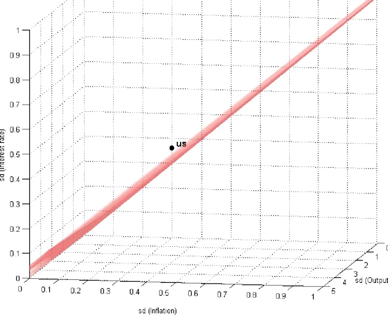
inflation persistence by setting γ = 0.5 and consider an economy with a distorted steady state, so that any shock will affect all the endogenous variables, and consider the time-consistent optimal policy. While this is a stylized model, it is widely used in theoretical and empirical work. Figure 3 plots Vo
(similar in shape to the plot in figure 2) together with the outcome (σπt, σyt, σit) for the US over the period 1984:1 - 2005:1. There is no combination of the volatility of exogenous shocks and policymaker preferences that could have generated the observed (σU S
πt , σ U S yt , σ
U S
it ) as an optimal policy outcome. Enlarging the parametric family of singular models leaves the result for the US sample un-changed. We build the function M (β; o) for β = [σat, στt, χ, γ, θ, ν]0 where χ is the share of firms that cannot optimally adjust the price in each period, γ is the fraction of last period’s aggregate inflation rate to which the share χ of firms indexes the price, θ is the firms’ demand elasticity, ν is the inverse of labor supply wage elasticity. We assume the policymaker maximizes the representative household’s utility. Table 1 reports the range of variation for the model’s parameters. The mapping still results in (σU Sπt , σU Syt , σU Sit ) /∈ Vo. 3 Including additional parameters in β may eventually result in a large enough
optimal policy space such that (σU S πt , σ
U S yt , σ
U S
it ) ∈ Vo, but does not need to because of the nonlinearity of the mapping M (β; o).
2Using β = [σ
at, σGt, στt, α]0 would generate the same image for M (β; o). To ease the reading of the plot in figure 2
the set Vo is defined in terms of the standard deviation of a variable rather than of its variance. 3
We verified that (σU Sπt, σ
U S yt , σ
U S
it ) /∈ Vo by searching for a vector β = [σat, στt, χ, γ, θ, ν, ]0 such that (σπt, σyt, σit)
is in the ±2.5% interval around the data point (σU S πt, σ
U S yt , σ
U S
it ). Allowing for a range of variation in (σπt, σyt, σit) lets
us account for the numerical error in the approximation to M (β; o). The map M (β; o) is computed through a discrete approximation over 3,686,000 simulated data points. We verified that admissable parameter values outside the range in table 1 result in outcomes further away from the historical observation for the US.
The result can be explained by two observations. First, all the model parameterizations imply different responses of endogenous variables to exogenous shocks. But many of the resulting models are nearly observationally equivalent in terms of unconditional volatility outcomes (σπt, σyt, σit). A measure of volatility is a coarse, low-level characterization of the behaviour of endogenous variables. What does change across model parameterizations is the mapping between the volatility of exogenous shocks and endogenous variables. That is, the same outcome (σπt, σyt, σit) can be generated with alternative parameterizations by different vectors [σat, στt, χ, γ, θ, ν]0. Second, changes in a parameter
do not necessarily add useful degrees of freedom to enlarge Vo. For example, in the optimal policy
space for (σπt, σhxt, σit) of the basic new Keynesian model a change in λ is observationally equivalent to a change in α, since the relationship between ext and πt and between xet and it in eqs. (7) and (8)
depends on the ratio α/λ.
The difficulty in finding a model within the parametric family such that the US outcome belongs to the optimal policy space has two alternative interpretations. First, US monetary policymaking was indeed suboptimal. After all, the building of the optimal policy space does allow for any possible parameterization in the vector [σat, στt, χ, γ, θ, ν]0, including parameterizations that may be inconsistent with available empirical evidence. Moreover, the optimal policy space has by construction weak power against detecting suboptimal policies: historical outcomes may belong to Vo even if they are the result
of period-by-period suboptimal policies. Finally, it can be shown that the outcome (σU Sπt , σU Syt , σU Sit ) does not belong to Vo for a number of alternative policies, including the timeless perspective optimal
commitment policy, or the policymaker adopting the the wrong objective function and assuming γ = 0 in eq. (5), or even the policymaker adopting an objective function quadratic in π, extand ∆it, for any
relative weight of the three objectives.
Second, the DSGE model propagation mechanism is incomplete or inaccurate. Conditional on optimal monetary policy, it puts implausible restrictions on the endogenous variables’ variances. This conclusion leads to question whether the optimal policy prescriptions derived from stylized DSGE models such as the one used are appropriate to guide real-world policymaking.
4
A Probabilistic Interpretation
Consider an optimal policy DSGE model with associated law of motion Z(β; o) described by the linear map Yt = AUt where A is an n × r matrix. Partition the vector β into βσ = [σU1,t, ...σUr,t] and βk= [k1, k2, ...ks]. It is assumed the matrix A is a function of βk, a vector of structural parameters of
the model.
In general, when r < n the support of the probability measure associated with the random vector Yt lies on an r−dimension hyperplane in Rn. The sample space Ωr is a null set with respect
to Lebesgue measure in Rn, and a density function is not defined with respect to the n−dimension
Lebesgue measure, while it exists with respect to Lebesgue measure in Rr for events belonging to
the r−dimension sample space Ωr. This is the relevant sample space for most DSGE models used in
business cycle analysis, and for every optimal policy model by construction, since optimal policy implies movements in the policy instrument can be written as a function of endogenous variables only, so that r < n.
If r < n and Ut is normally distributed, the random vector Yt is said to have a singular normal
distribution. With a slight abuse of notation, we can write Yt∼ Nn[AμU, AΣUA0]. A singular normal
distribution has a covariance matrix with rank strictly smaller than the dimension of the random vector.
4 To each parameter vector β
k corresponds a null set Ωr(βk) in Rn. Since the sample space Ωr is not
a function of βσ, a set Vo(βk) = M (βk, βσ; o) can be associated with Ωr(βk). Section 2 showed that
Vo(βk) and Ωr(βk) have the same dimension, since if Yt has singular covariance matrix with rank r,
the set Vo(βk) is a r-dimension hyperplane in Rn.
The space Vo encompasses all sets Vo(βk) for any parameterization of the vector βk. Notice
that since Vo simply maps entries of A and ΣU into ΣY, the set Vo can be built regardless of the rank
of ΣU. On the contrary, we cannot define a joint density for the model Z(β; o) since the sample space
is the null set in Rn, nor can we write a likelihood function for an observed sample.
A vector ΣY in Rn belonging to Vo must also belong to Vo(βk) for some βk, and therefore ΣY is
the outcome of an optimal policy singular model. A model may impose restriction on ΣU, for example
requiring that the structural shocks Ut be uncorrelated, and ΣU diagonal. The set Vo satisfying these
restrictions is thus the population optimal policy space. If the vector βσ includes all the elements of ΣU
we can build a sample optimal policy space, and incorporate the impact of small sample uncertainty. In the example discussed in section 3, assuming β = [σat, στt, σatτt, α]0 implies the set Vo includes all the realizations of the random vector (σπt, σyt, σit) for any possible sample draw from the distribution of the random vector Ut, regardless of the population value for ΣU. Therefore Vo is the space of all
possible sample outcomes (Sπt, Syt, Sit) for (σπt, σyt, σit). If a sample observation (Sπt, Syt, Sit) does not belong to Vo, then the sample {Yt}Tt=0 does not belong to the sample space Ωr(βk) for any βk.
4While a likelihood function for Y
t does not exist, various authors have proposed methods for maximum likelihood
The optimal policy space depicted in figure 3 is in fact drawn without imposing any restriction on ΣU. The result implied by figure 3 that (SπU St , S
U S yt , S
U S
it ) /∈ Vo has the interpretation that the sample {πt, yt, it}Tt=0 such that (Sπt, Syt, Sit) = (S
U S πt , S
U S yt , S
U S
it ) does not belong to the sample space of the data-generating process in eqs. (3), (4), (5) for all possible values of the preference parameter α. An equivalent way of stating the same result is that, while unconditionally the probability of any draw for (σπt, σyt, σit) is always nonzero (and a confidence ellipse could be computed using standard statistical results for random sampling), no amount of sampling uncertainty could have generated the draw (SπU St , SyU St , SU Sit ) conditional on our assumptions for the data generating process. Whatever the amount of sampling uncertainty, and the true population value for (σπt, σyt, σit), the data imply the model is false: either the propagation mechanism in eqs. (3), (4) is mistaken, or the policymaker deviated from the optimal policy in a way that the optimal policy space is able to discriminate.
The set Vo computed earlier for β = [σat, στt, χ, γ, θ, ν]0 imposed the restriction that ΣU be diagonal, thus it did not include all possible sample outcomes (Sπt, Syt, Sit). Building Vo ac-counting for sample uncertainty is straightforward, but computationally burdensome. For the case β = [σat, στt, χ, γ, θ, ν]0 we perform a different exercise, that illustrates the impact of the covariance matrix singularity on the optimal policy space. Assume the observable interest rate iobst is described by
iobst = it+ wt
where wtis random variable with variance σ2wt = x 100σ
2
it. The value x gives the variance of the variable wt as a percent share of the variance of the unobservable variable it, which is assumed to behave according
to the optimal policy. In the econometric literature wt is assumed to represent a measurement error.
It can be interpreted as summarizing the volatility in iot which is not explained by the DSGE model. By adding a third source of randomness, we enlarge the set Vo of optimal policy outcomes, and
obtain a measure of how large deviations of the observed σit from the volatility implied by the optimal policy need to be to have a nonzero probability of observing a given (σπt, σyt, σit) conditional on the data-generating process in eqs. (3), (4), (5) and on all possible vectors β = [σat, στt, σwt, χ, γ, θ, ν]0.
Given our model, we can now ask what is the probability of a population value (σπt, σyt, σit) equal to the US observation and belonging to Vofor different values of x. The probability is calculated for
the standard deviation of a variable ztbelonging to the 5% interval [bLzt,U S, bHzt,U S] centered around the
observation SzU St . Finally, let Voi ⊆ R+ be the optimal policy space for the variable it and Voπ,y⊆ R2 +
of an outcome σit ∈ [b L it,U S, b H it,U S] belonging to V i
o conditional on any value within the 5% interval for
(σπt, σyt) belonging to V π,y o . Formally, we compute Pr ⎧ ⎨ ⎩ h (σit ∈ V i o) ∩ (bLit,U S ≤ σit ≤ b H it,U S) i | [(σπt, σyt) ∈ V πy o ∩ (bLπt,U S ≤ σπt ≤ b H πt,U S) ∩ (b L yt,U S ≤ σyt ≤ b H yt,U S)] ⎫ ⎬ ⎭
Figure 4 plots the conditional probability against the variance σ2wt as a percent share x of the variance σ2it. Allowing for a third source of randomness implies that the US observation outcome can be the result of optimal policymaking, even without allowing for sampling uncertainty. The variable x provides a simple measure of the additional randomness needed for the US observation to belong to Vo.
5
Related Literature
A growing literature investigates the fit of micro-founded DSGE models to the data conditional on an optimal monetary policy. Research focused on forward and backward-looking small macroeconomic models used in monetary policy work. Soderstrom et al. (2002) use informal calibration to match a new Keynesian model dynamics to US data. Dennis (2004), Favero and Rovelli (2003) and Salemi (2006) estimate structural models subject to the restriction that the policy rule minimizes the policymaker loss function.
Given a time series for the observables (Y1t...Ynt) with covariance matrix ΣY the approach adopted by these authors produces estimates for the deep parameters, the policymaker preferences, and a time series for a vector of shocks with nonsingular covariance matrix such that the theoretical model can generate the historical data, and such that a given function, depending on the econometric technique adopted, is maximized. This also implies that there will exist an estimated parameter vector, including random deviations from the optimal policy, such that the historical volatility outcome can be generated by the model.
Salemi (2006) shows how to use the nonsingular model estimation approach to compute a statistical test for optimal policymaking. The optimal policy imposes cross-equation restrictions on the estimated parameters, and their impact on the likelihood of the model can be exploited for testing. The optimal policy space is instead built exploiting the restrictions imposed by truly optimal policymaking in a parametric family of singular models on the volatility of observable variables. Compared to the estimation assumptions, the singular-model approach makes stronger assumptions on the behaviour
of the policymaker, who is assumed to always implement the optimal policy. On the other hand, it relaxes the demand on the data fit since policies that are period-by-period suboptimal may still result in volatility outcomes belonging to the optimal policy space.
Clearly a three-equations model, as the one adopted in this paper, can only provide a stylized description of the economy’s behaviour. Yet small optimal policy DSGE models are estimated to gain insight into the preferences of the policymaker, and are often relied upon by economists to illustrate and generate policy prescriptions and guidelines. Computing the optimal policy space for such models provides important insights into the restrictions on the data that the models imply.
6
Conclusions
This paper studied the restrictions implied by optimal policy DSGE models for the volatility of ob-servable endogenous variables.
Our approach relies on the restrictions imposed by optimal policymaking on the variance of the endogenous variables in singular models. To generate a non-trivial set for the volatility of observable variables - which we label the optimal policy space - we introduce variation in the behavioral parameters when building the set of outcomes consistent with the model. We show that a DSGE model can be associated with a well-defined subset of all the possible volatility outcomes, which is not of measure zero. This is the result of the nonlinearity of the mapping between a DSGE model parameter space and the implied volatility of the endogenous variables. Nonsingular models, which assume random perturbations to optimal policymaking, imply no observable outcome has zero probability.
We illustrated our method by building the optimal policy space of a widely used new Keynesian model. Conditional on this model, recent US monetary policymaking would have zero likelihood of being the result of optimal policymaking. Since this approach has by construction low power in discriminating optimal policy outcomes, we interpret the result as evidence that widely used optimal policy models can only be consistent with a very limited set of volatility outcomes, regardless of the parameterization adopted.
References
[2] Benigno, P. and Woodford, M., (2005), ”Inflation Stabilization and Welfare: the Case of a Distorted Steady State”, Journal of the European Economic Association 3(6): pp. 1185-1236.
[3] Bierens, H., (2007) "Econometric analysis of linearized singular dynamic stochastic general equi-librium models", Journal of Econometrics 136: pp. 595-627.
[4] Clarida, R., Galí, J., and M. Gertler, (1999), “The Science of Monetary Policy: A New Keynesian Perspective,” Journal of Economic Literature, 37, 4, pp. 1661-1707.
[5] Conlon, L., (2001), Differentiable Manifolds, Boston: Birkhauser.
[6] Dennis, R., (2004), ”Inferring Policy Objectives from Economic Outcomes”, Oxford Bulletin of Economics and Statistics 66: pp. 735-764.
[7] Favero, C. and Rovelli, R., (2003), ”Macroeconomic Stability and the Preferences of the Fed: A Formal Analysis, 1961-1998”, Journal of Money, Credit and Banking 35: pp. 546-556.
[8] Kwakernaak, H., (1979), "Maximum likelihood parameter estimation for linear systems with sin-gular observations", IEEE Transactions on Automatic Control AC-24:3.
[9] Lai, Hung-pin, (2008), "Maximum likelihood estimation of singular systems of equations", Eco-nomic Letters 99: pp. 51-54.
[10] Salemi, M., (2006), ”Econometric Policy Evaluation and Inverse Control”, Journal of Money, Credit and Banking 38: pp. 1737-1764.
[11] Soderstrom, U., Soderlind, P. and Vredin, A., (2002), ”Can a Calibrated New -Keynesian Model of Monetary Policy Fit the Facts?”, Sveriges Riksbank Working Paper 140.
[12] Walsh, C., (2005), ”Endogenous Objectives and the Evaluation of Targeting Rules for Monetary Policy”, Journal of Monetary Economics 52: pp. 889-911.
New Keynesian model parameter range for US optimal policy space
γ χ v θ
0.2-0.82 0.1-0.66 0.1-1.17 4-16
Table 1:New Keynesian model parameter space used to compute optimal policy spaceVo = M (β; o)
for β = [σat, στt, χ, γ, θ, ν]0.Other parameters are set as in Walsh (2005). Model is described by the
time-consistent solution to maximization of eq. (5) given eqs. (3), (4) and assuming the policymaker’s objective function maximizes the utility of the representative household.Parameter χ is the share of firms that cannot optimally adjust the price in each period,γis the fraction of last period’s aggregate inflation rate to which the shareχof firms indexes the price,θis the firms’ demand elasticity,νis the inverse of labor supply wage elasticity. Parameter values outside the range in table 1 result in outcomes(σπt, σyt, σit) further from the historical US
0 0.1 0.2 0.3 0.4 0.5 0.6 0.7 0.8 0.9 0 0.05 0.1 0.15 0.2 0.25 0.3 0.35 0 0.1 0.2 0.3 0.4 0.5 0.6 0.7
Variance (output gap)
Optimal policy space for σ π 2 , σx2 , σi2
Variance (inflation)
lower bound for σi2
lower bound for σi2
lower bound for σi2
lower bound for σi2
V ar ian ce ( in ter es t r a te)
Figure 1: Sample optimal policy hyperplanes in the optimal policy space Vo for the variables
(πt,xet, it) and for β = [σ2ut, σ 2 h rn
t, α]
0 using the baseline new Keynesian model. Each hyperplane is
indexed by a value for σ2hrn t.
0 1 2 3 4 5 6 7 8 0 0.05 0.1 0.15 0.2 0.25 0.3 0.35 0 0.05 0.1 0.15 0.2 0.25 0.3 Variance (inflation) Optimal policy space for σ π 2 , σy2 , σi2
Variance (output) V ar ia nce ( int e res t ra te )
Figure 2: A subset of the optimal policy space Vo for the variables (πt, yt, it) and for
β = [σ2ut, σ2hrn t, α]
Figure 3: A subset of the optimal policy space Vo for the variables (πt, yt, it) and for
β = [σ2ut, σ2hrn t, α]
0 using a new Keynesian model with endogenous inflation persistence and a distorted
steady state. The plot shows the historical volatility outcome for the US over the period 1984:1 -2005:1. Output ytis detrended seasonally adjusted non-farm business sector real GDP. Inflation πtis
seasonally adjusted CPI inflation. Interest rate itis 3-month government bond. All data is sampled
0 10 20 30 40 50 60 70 80 90 100 0 0.1 0.2 0.3 0.4 0.5 0.6 0.7 0.8 0.9 1
Interest rate measurement error variance - percent share
Li kel iho od Probability of US outcome (σ π 2 , σ y 2 , σ i
2) belonging to optimal policy space
Figure 4: Probability of the outcome
{(bLit,U S ≤ σit ≤ b H it,U S) ∩ (b L πt,U S ≤ σπt ≤ b H πt,U S) ∩ (b L yt,U S ≤ σyt ≤ b H
yt,U S)} belonging to the optimal policy space Vo, conditional on the outcome {(bLπt,U S ≤ σπt ≤ b
H πt,U S) ∩ (b L yt,U S ≤ σyt ≤ b H yt,U S)} belonging to the optimal policy space Voπ,y. Horizontal axis measures variance of the measurement
error for observed interest rate iobst as a percent share of the variance for the optimal interest rate it,
7
Appendix: Solution of the Benigno and Woodford (2005) Model
Consider the New Keynesian model for inflation πt, output gap xt, interest rate itas described in Walsh
(2005) and Benigno and Woodford (2005):
xt = − 1 ϕ(it− Etπt+1− r n t) + Et(xt+1) (11) πt− γπt−1 = λxt+ eβEt(πt+1− γπt) (12) xt = yt− ynt where rn
t is the Wicksellian real rate of interest, yt is output, ynt is the level of output that would
obtain in the flexible-price equilibrium, ϕ is the coefficient of relative risk aversion for the representative household divided by the consumption share of output, eβ is the household’s discount rate. It is assumed that a constant share of firms can adjust the price in each period, while the remaining share indexes the price to a fraction γ of last period’s aggregate inflation rate. When prices can optimally adjust in every period the rational expectation equilibrium solution for ytn and rnt does not depend on it:
ynt = φ1Gt+ φ2at+ φ3τt rnt = φ4Et(yt+1n − ynt) + φ5Et(Gt+1− Gt) φ1 = ϕ ω + ϕ φ2 = ζ(1 + v) ω + ϕ φ3 = [τ /(1− τ)] ω + ϕ φ4 = ϕ φ5 = (1 − sC) ω = ζ(1 + v) − 1
The variable Gt is defined as exogenous government consumption (in log-deviations from the
steady state), at is an exogenous productivity shock, τt is an exogenous income tax shock. The
parameter ζ is the elasticity of firm output with respect to labor input, v is the inverse of the wage elasticity of labor supply, ω is the inverse of the elasticity of firm marginal cost with respect to output, τ is the steady state tax rate, sC is the consumption steady state share of output, ϕ is the coefficient
of relative risk aversion for the representative household divided by sC. The elasticity of inflation with
respect to xt is given by:
λ = (1 − χ)(1 − χeβ)
χ(1 + θω) (ω + ϕ)
In the absence of transfers to correct the steady state distortions arising from taxes and imperfect competition, or in the case τt6= 0, the efficient level of output y∗ is different from yn and is given by:
yt∗ = w1ynt + w2Gt+ w3τt w1 = ω + ϕ + Φ(1 − ϕ) ξ w2 = Φσ (ω + ϕ)ξsC w3 = τ /(1 − τ)ξ ξ = (ω + ϕ) + Φ(1 − ϕ) −Φσ(s −1 C − 1) (ω + ϕ) Φ = 1 − θ − 1 θ (1 − τ)
where θ is the firms’ demand elasticity. The second order approximation to the utility of the household can be written as:
Wt = − 1 2ΩEt ∞ X i=0
eβi©αex2t+i+ (πt+i− γπt+i−1)2
ª
(13) e
xt = (yt− y∗t)
wherexet is the welfare-relevant output gap. Wtis equal to the household’s welfare for α = α∗
where
α∗ = λ
w1θ
objective function (13): e xt = − 1 ϕ(it− Etπt+1− er n t) + Et(xet+1) (14) πt− γπt−1 = λxet+ eβEt(πt+1− γπt) + λut (15) ern t = φ4Et(yt+1∗ − yt∗) + φ5Et(Gt+1− Gt) ut = y∗t − ytn
The variable utis a linear combination of all the exogenous shocks. The variable Φ is a measure
of the steady state distortions in the economy. If appropriate transfers ensure, as is often assumed, that the steady state is efficient, then Φ = 0. Benigno and Woodford (2005) show that in this case w1= 1, w2= 0, and
ut= w3τt
Assume γ = 0. Then the problem faced by the optimal policymaker can be written as:
M ax −12ΩEt ∞ X i=0 e βi©αxe2t+i+ π2t+iª (16) st xet = − 1 ϕ(it− Etπt+1− er n t) + Et(xet+1) (17) πt = λxet+ eβEtπt+1+ λut (18) ut = w3τt (19) ernt = φ4Et ∙ ϕ(Gt+1− Gt) + ζ(1 + v)(at+1− at) ω + ϕ ¸ + φ5Et(Gt+1− Gt) (20)
In this model movements in at or Gt can be interpreted as ’demand shocks’ since they affect
ern
t but not ut, therefore do not affect the trade-off between the stabilization objectives and can be
perfectly offset by the policymaker. The variable ut takes the interpretation of a ’cost push’ shock,
at= ρaat−1+ εat, εt ∼ iid , ρG= ρa it holds: ertn = φ4Et(yt+1∗ − y∗t) yt∗ = − 1 ϕ(1 − ρa)er n t (21)
Eq. (21) holds also for sC < 1 and Gt= 0 ∀ t or for sC < 1 and ρg = 1.
The optimal time-consistent policy is given by the FOC:
πt− γπt−1= −
α
λ(1 + eβγ)xt
The timeless perspective optimal commitment policy is given by the FOC:
πt− γπt−1=
³ −αλ
´
(xt− xt−1)
Baseline parameterization The parameterization follows Walsh (2005) unless otherwise stated in
the main text.
χ = 0.66 γ = 0.5 e β = 0.99 ϕ = 0.16 φ = 1.5 θ = 7.88 sC = 0.8 v = 0.49 τ = 0.2 ρa = 0.95 ρG = 0.95 ρτ = 0.95
![Table 1: New Keynesian model parameter space used to compute optimal policy space V o = M (β; o) for β = [σ a t , σ τ t , χ, γ, θ, ν] 0](https://thumb-eu.123doks.com/thumbv2/123doknet/7711596.247364/17.918.197.716.149.211/table-keynesian-model-parameter-space-compute-optimal-policy.webp)