HAL Id: hal-01858321
https://hal.univ-lorraine.fr/hal-01858321
Submitted on 30 Apr 2019
HAL is a multi-disciplinary open access
archive for the deposit and dissemination of sci-entific research documents, whether they are pub-lished or not. The documents may come from teaching and research institutions in France or abroad, or from public or private research centers.
L’archive ouverte pluridisciplinaire HAL, est destinée au dépôt et à la diffusion de documents scientifiques de niveau recherche, publiés ou non, émanant des établissements d’enseignement et de recherche français ou étrangers, des laboratoires publics ou privés.
KG
2B, a collaborative benchmarking exercise for
estimating the permeability of the Grimsel
granodiorite-Part 2: modelling, microstructures and
complementary data
C David, J Wassermann, F Amann, J Klaver, C Davy, J Sarout, L Esteban, E
Rutter, Q Hu, L Louis, et al.
To cite this version:
C David, J Wassermann, F Amann, J Klaver, C Davy, et al.. KG2B, a collaborative benchmarking
exercise for estimating the permeability of the Grimsel granodiorite-Part 2: modelling, microstructures and complementary data. Geophysical Journal International, Oxford University Press (OUP), 2018, 215 (2), pp.825 - 843. �10.1093/gji/ggy305�. �hal-01858321�
1 2 3 4 5
KG²B, a collaborative benchmarking exercise
for estimating the permeability of the Grimsel granodiorite:
modeling, microstructures and complementary data
C. David1, J. Wassermann2, and the KG²B Team3*
6 7
1
Université de Cergy-Pontoise, Laboratoire GEC, Cergy-Pontoise, France.
8 2
Université de Cergy-Pontoise, Laboratoire L2MGC, Cergy-Pontoise, France.
9 3
Complete list detailed in Appendix A.
10 11
Corresponding author: Christian David ([email protected])
12 13
Key Points:
14
• A benchmarking exercise involving 24 laboratories was organized to estimate the
15
permeability of the Grimsel granodiorite
16
• The microstructures of the Grimsel granodiorite were analyzed and quantified using
17
BIB-SEM, micro-CT scanning, MICP and NMR techniques
18
• Permeability predictions from different models using microstructure data as input
19
parameters are in good agreement with measurements
20 21
Abstract
22
A benchmarking exercise involving 24 laboratories was organized for measuring and
23
modeling the permeability of a single low permeability material, the Grimsel granodiorite. To
24
complement the data set of permeability measurements presented in a companion paper, we
25
focus here on (i) quantitative analysis of microstructures and pore size distribution, (ii)
26
permeability modeling and (iii) complementary measurements of permeability anisotropy and
27
poroelastic parameters. BIB-SEM, micro-CT, MICP and NMR methods were used to
28
characterize the microstructures and provided the input parameters for permeability
29
modeling. Several models were used: (i) basic statistical models, (ii) 3D pore network and
30
effective medium models, (iii) percolation model using MICP data and (iv) free-fluid model
31
using NMR data. The models were generally successful in predicting the actual range of
32
measured permeability. Statistical models overestimate the permeability because they do not
33
adequately account for the heterogeneity of the crack network. Pore network and effective
34
medium models provide additional constraints on crack parameters such as aspect ratio,
35
aperture, density and connectivity. MICP and advanced microscopy techniques are very
36
useful tools providing important input data for permeability estimation. Permeability
37
measured ~orthogonal to foliation is lower that ~parallel to foliation. Combining the
38
experimental and modeling results provides a unique and rich data set.
39 40
1. Introduction
41
Following a workshop on «The challenge of studying low permeability materials»
42
that was held at Cergy-Pontoise University in December 2014, a benchmark exercise in
43
which several laboratories estimate the permeability of a single material was proposed to the
44
attendees. The selected material was the Grimsel granodiorite (Switzerland) and the
45
benchmark was named the “KG²B” project, from “K for Grimsel Granodiorite Benchmark”
46
(David et al., 2017). Multiple objectives were defined: (i) to compare the results for a given
47
method, (ii) to compare the results between different methods, (iii) to analyze the accuracy of
48
each method, (iv) to study the influence of experimental conditions (especially the nature of
49
pore fluid), (v) to discuss the relevance of indirect methods and models, and finally (vi) to
50
suggest good practice for low permeability measurements. The permeability measurements
51
are presented in the companion paper. Here we will focus on item (v) and present the results
52
of microstructure analyses and permeability modeling.
53
Fluid flow processes in rocks are controlled by the geometrical properties of pore
54
and/or cracks and the topology of the pore/crack network. Linking permeability to
55
microstructural properties has always been a challenge in rock physics. A first step is to
56
acquire high quality data that allow thorough characterization of the pore space, preferably in
57
3D. As we are dealing with a crystalline rock, the focus is on cracks rather than pores. Cracks
58
in rocks can be approximated as planar features with small width or aperture, randomly
59
oriented or not in a 3D medium. Due to their limited resolution, optical microscopy
60
techniques are not well-suited for the study of cracks. SEM studies have been commonly
61
used to analyze cracks on thin-sections at high magnification. Ion beam milling is
62
recommended to avoid biased interpretation of the microcrack morphology and statistics
63
(Wong, 1982). Crack statistics provided by SEM studies can be from 2D analyses, from
64
which 3D parameters (like crack surface per unit volume) can be inferred using stereology
65
(Fredrich & Wong, 1986). Recent advances in ion polishing now allow improved images of
66
pore structures and crack networks to be obtained using BIB-SEM (Klaver et al., 2015), or
67
even 3D structures from FIB-SEM image stacks (Holzer et al., 2004). Wood’s metal injection
into the pore space greatly enhance pore and crack detection and analysis on SEM images
69
(Hu et al., 2012; Klaver et al., 2015). High resolution micro-CT techniques have become
70
widely used to investigate the three-dimensional distribution of minerals and pores (Baker et
71
al., 2012; Godel, 2013). With improvement of technology and analytical tools, sub-micron
72
resolution can now be achieved with micro-CT imaging methods, but sometimes even this is
73
insufficient to identify tiny cracks in crystalline rocks. One major advantage of micro-CT is
74
that the technique is non-destructive and can be applied on centimeter scale plugs. Pore or
75
crack size distributions can be obtained by image analysis on SEM images (2D analysis) or
76
micro-CT reconstructed volumes (3D analysis), and also by conducting mercury injection
77
capillary pressure (MICP) tests on small plugs. MICP is commonly used in petrophysical
78
studies to obtain the throat size distribution and capillary breakthrough pressure by injecting
79
mercury under increasing pressure (Hu et al., 2015). The throat size distribution given by
80
MICP does not actually match the pore size distribution of the rock because of constrictions
81
and ink-bottle effects in the pore space (Abell et al., 1999) but provides a first-order
82
approximation that can be used in models. Other methods that provide insight into the pore
83
size distribution include the gas adsorption (or BET) method (Schull, 1948) and NMR
84
techniques (Josh et al., 2012).
85
Permeability models using microstructural data as input parameters have evolved
86
since the pioneering work of Kozeny in the 1920s (Kozeny, 1927). A main challenge of all
87
permeability models is to identify the characteristic length scale controlling permeability.
88
This general statement rises from the permeability having the unit of squared length, but
89
other factors like pore size variability and connectivity are also very important. Many
90
different approaches have been proposed (Guéguen & Palciauskas, 1994). Originally based
91
on the Kozeny-Carman equation (Kozeny, 1927), the equivalent channel model states that the
92
characteristic length scale is the hydraulic radius, defined as the ratio between the pore
93
volume and the pore surface area (Paterson, 1983; Walsh & Brace, 1984). In the equivalent
94
channel model, permeability depends on bulk properties related to the pore space (volume to
95
surface ratio, porosity, tortuosity - an ill-defined parameter related to the increased path
96
length in a “tortuous” pore space) that, with the exception of tortuosity, are measurable at the
97
sample scale. Statistical and effective medium models take advantage of the statistics of pore
98
or crack geometries. For example, Gueguen & Dienes (1989) proposed a statistical model for
99
crystalline rocks in which permeability depends on the mean crack aperture and radius, with
100
cracks modeled as penny-shaped objects, on the average distance between cracks and on the
101
fraction of connected cracks (which can be estimated from percolation theory). Only
102
ensemble averages are estimated with limited input of the crack network topology. In
103
contrast, network topology is taken into account in percolation and network models. For the
104
percolation model proposed by Katz & Thompson (1986) the characteristic length scale is the
105
so-called critical conductance (linked to a critical crack size), defined as the smallest
106
conductance in the sample-spanning sub-network made of conductances larger than the
107
critical conductance. The critical length scale can be obtained from the breakthrough pressure
108
in MICP experiments using Washburn’s equation (Hu et al., 2015). Percolation models are
109
supposed to work best when the pore size distribution is very wide. In heterogeneous porous
110
media, preferential flow paths (with similar properties as the critical percolation subnetwork)
111
are more likely to occur (David, 1993).
112
Pore network modeling has been widely used for permeability prediction (Bauer et al.,
113
2012; Bernabé et al., 2003). In such models fluid flows in pipes or cracks forming the bonds
114
of a 3D (or 2D) lattice with fixed topology (e.g. a cubic lattice). The geometrical properties of
115
the conducting elements follow the pore/crack size statistics obtained by SEM analysis or
MICP (David et al., 1990). The flow equations are solved at each node and permeability is
117
directly derived from Darcy’s law, so does not depend on statistical averages (De Boever et
118
al., 2012). Pore network modeling also allows the bond occupancy probability to be varied,
119
so that networks with different average coordination number (or connectivity) can be
120
considered for permeability estimation (David, 1993). Several of the permeability models
121
mentioned above were tested by Casteleyn et al. (2011) on series of oolitic limestones from
122
the Paris basin. Since the pore size distribution of these rocks was not very heterogeneous,
123
hence statistical and network models were successful in matching the measured permeability,
124
while the percolation model underestimated the permeability by about one order of
125
magnitude.
126
One of the objectives of the KG²B benchmark was to conduct permeability modeling.
127
Several models were selected by the participants. To achieve successful modeling, as
128
discussed above, information is required about the rock microstructure (such as porosity,
129
pore/crack aperture and length distribution, and connectivity). We will present the results of a
130
thorough microstructural analysis and from NMR and MICP tests, as well complementary
131
data on anisotropy and poroelastic parameters measured on a voluntary basis by some
132
participants.
133 134
2. The KG²B Project: Summary
135
In total 30 laboratories from 8 different countries volunteered to participate in KG²B,
136
and we received results from 24 laboratories that form the “KG²B Team”. The complete list
137
of participants who sent results is given in Appendix A. A dedicated website
https:/labo.u-138
cergy.fr/~kggb/ was created with information on the benchmark, including a web page where
139
the progress of the project could be followed on the “KG²B-wheel”, which was updated as
140
soon as results were received from any of the participants. It took one year to collect all of the
141
results. In total we collected 45 permeability values, including 39 measured values and 6
142
results from modeling, on which this paper will focus. Statistical, network, percolation and
143
effective medium models were used. We add a seventh modeling result in which a rock
144
sample is treated as an RC (Resistance + Capacitor) low pass filter during pore pressure
145
oscillation tests.
146
The Grimsel granodiorite was obtained from the Swiss Grimsel test site, a 450 meter
147
deep Underground Research Laboratory (URL). The 950 meter long and 3.5 meter diameter
148
tunnels were excavated in 1983 by a full face Tunnel Boring Machine (TBM) in hard rocks,
149
mainly granite and granodiorite, at an altitude of 1730 m in the Central Aar Massif in
150
Switzerland. The TBM excavation method limited perturbation of the host rock, with a quite
151
small Excavation Damage Zone (EDZ) around the tunnel (Egger, 1989). Along the tunnel,
152
major damage zones are located in meter scale shear zones or widely spaced discontinuities
153
caused by regional deformation. Two cores of Grimsel granodiorite, each about one meter
154
long and of diameter 85 mm, were provided by our Swiss colleagues in September 2015.
155
These cores were retrieved at a distance of 4 to 6 meters from the tunnel of the Grimsel test
156
site, far away from the EDZ influence. The cores were cut into small blocks at lengths
157
requested by each participant (between 2 and 10 cm). A grain shape foliation is visible on the
158
cores at an angle of about 20-30° with respect to the core axis. The foliation is related to
159
compositional banding of alternating dark biotite layers and quartz-rich layers (Schild et al.,
160
2001). Natural and induced cracks have been observed in past studies (e.g. Smith et al.,
161
2001). In particular there is a natural interconnected network of cracks producing about 1%
porosity in the granitic matrix. Stress release due to drilling and sample preparation outside
163
the URL seems to be responsible for larger micro-crack apertures than those observed
164
directly in situ (Schild et al., 2001). As some laboratories provided permeability
165
measurements in directions other than that required of the participants (i.e. the core axis
166
direction), we will also discuss the permeability anisotropy.
167
The detailed analysis of the permeability measurements is given in the companion
168
paper. Let us recall the most important results. For the whole data set of 39 measurements,
169
the average permeability was 1.47 10-18 m²; however 4 outliners were identified and removed,
170
leading to an average permeability of 1.11 10-18 m² and a standard deviation of 0.57 10-18 m².
171
A striking result was the large difference between measurements using gas or liquid as the
172
pore fluids: the permeability to gas was about twice as large as the permeability to liquid
173
(kgas=1.28 10-18 m², kliquid=0.65 10-18 m²). The model predictions presented in this paper will
174
be compared to those values.
175
We will use the same convention as in the companion paper for presenting the data
176
set. Each lab was assigned a number in increasing order with respect to the distance between
177
their sample and the tunnel. Lab#01 worked on the sample closest to the tunnel, and Lab#24
178
on the farthest sample.
179 180
3. Microstructure and porosity analyses
181
3.1. Quantitative Microstructural Analysis
182
Here we describe efforts to determine the main fluid flow pathways at the centimeter
183
scale, which is the relevant scale for the laboratory experiments. To this purpose, several
184
direct imaging methods were used: automated optical microscopy of thin-sections, and Broad
185
Ion Beam/Scanning Electron Microscopy (BIB-SEM) of intact or Wood’s Metal (WM)
186
impregnated samples.
187
3.1.1 Methods 188
Two adjacent blue dye impregnated thin-sections of standard size were prepared
189
perpendicular and parallel to the core axis from the original core sample (Figure 1).
Thin-190
sections were automatically scanned with the Virtual Petroscan (ViP) (Schmatz et al., 2010)
191
in plane polarized and crossed polarized light (PPL and XPL). Porosity was segmented from
192
the PPL image map (approximately 20,000 * 12,000 pixels, pixel size of 1.4 µm i.e. 2.8 cm *
193
1.68 cm ≈ 4.7 cm2
) by unsupervised iso-cluster classification and re-grouped into porosity
194
and matrix based on visual inspection followed by a boundary cleaning operation (dilation),
195
all in ArcGIS 10.
197
Figure 1. Grimsel granodiorite core (left) and sampling (right) for thin sections perpendicular (1), and parallel
198
(2) to the core axis, for BIB-SEM and WM (3), and plug for permeability measurements for Lab#23 (4). 199
From the same core sample, one subsample was prepared by BIB polishing to investigate the
200
microstructure by SEM. Details on this technique are given by Klaver et al. (2012). Four
201
areas were mapped at high resolution (10,000 – 20,000 x magnification) for quantitative
202
analyses of the pore space. Porosity was segmented by a seed-and-grow algorithm (Jiang et
203
al., 2015) and manually corrected where needed. Pore spaces with circularity below 0.2 and
204
an axial ratio above 3 were automatically classified as cracks (including grain boundary
205
cracks). Average crack intensity (expressed in crack number/m) and average crack thickness
206
were calculated based on each pixel row from every map.
207
Another sub-sample was injected at 500 MPa with Wood’s metal (WM), which is a
non-208
wetting alloy with wetting properties similar to mercury and which solidifies at room
209
temperature. This method resembles Mercury Intrusion Porosimetry (Klaver et al., 2015). We
210
expected insignificant damage to the pores due to the material strength.
211
3.1.2 Visible porosity and pore size distributions 212
Over 60,000 pores were segmented from the thin-sections and the largest pores were
213
approximately 0.3 millimeter in equivalent diameter (Figure 2). The thin-sections show
214
different visible porosities: 0.71% and 1.55% for the parallel and perpendicular sections,
215
respectively. This difference most likely occurred because the thin-sections are not wholly
216
representative at the centimeter scale regarding porosity. Alternatively, this contrast may owe
217
to highly anisotropic pore shapes with large pore diameters parallel to the section and small
218
diameters perpendicular to the section.
219 220 221
Figure 2. ViP XPL maps overlain by pore segmentation in red of the parallel thin-section (A) and perpendicular
223
thin-section. The insets show the blue dye filled pores in PPL. 224
From SEM, the weighted average porosity in segmented maps perpendicular to the core
225
direction is 0.45% with a porosity of 0.54%, 0.16%, 0.64% and 0.39% in maps A, B, C and
226
D, respectively (Figure 3A-D). However, most of the pore space (average 0.36%) is
227
associated with cracks, indicated in red in the figure. In map D, no cracks were counted, and
228
all pores are interpreted as isolated pores within a single phase consisting mainly of K, Si, Al
229
(Figure 3E) and interpreted as K-feldspar. Other pore space-mineral associations are: 1)
230
cracks at grain boundaries and within biotite (Fe, K, Mg, Al, Si); 2) minor pores and cracks
231
along albite/plagioclase (Na/Ca, Al, Si) grain boundaries; 3) pores and cracks at quartz (Si,
232
O) grain boundaries and fluid inclusions; and, 4)fluid inclusions in apatite (Ca, P).
233 234
235
Figure 3. Backscattered Electron (BSE) image maps with pore space segmentation of maps A-D. Interpreted
236
cracks are in red and pores in cyan. The EDS (Energy Dispersive Spectroscopy) overview map shows the 237
locations of the maps with respect to BIB cross-sections and elemental compositions (E). 238
The pore size distributions (PSDs) of the imaged thin-sections show a clear increase in pore
239
frequency with decreasing equivalent diameter to about 6 µm (Figure 4A). The PSDs of the
240
BIB-SEM maps show a clear peak at 200 - 300 nanometer equivalent diameter and another
241
apparent increase below 100 nanometers. These smaller segmentations are below 18 pixels in
242
size. They are interpreted as noise and hence excluded from the analyses in Figure 4B, which
shows normalized frequencies (number of pores divided by the imaged area and bin width).
244
Taking into account both pores and interpreted cracks, only maps B and C show comparable
245
best fits. The fact that the normalized PSDs do not show uniform best fits indicates that pore
246
space may have been underestimated due to the large grain sizes and other heterogeneities.
247
Considering only the interpreted cracks in red (Figure 3A-D), the average crack thickness is
248
283 nm, within the visible range in Figure 4A. The average crack intensity over maps A-C is
249 14749 cracks/m. 250 251 252 253
Figure 4. A) PSDs of segmented porosity in the thin-sections and BIB-SEM maps. B)Plot showing the PSDs, 254
normalized over the imaged area for all segmented pores above 18 pixels in size, i.e. 6.5 µm, 144 and 72 nm for 255
the thin-sections, map A-C and map D respectively. 256
3.1.3 Pore connectivity 257
The WM-filled cross-section is shown in Figure 5; the minerals are mostly biotite,
258
albite, plagioclase and quartz (Figure 5A). Most of the WM is located in the cracks. Most of
259
the WM-filled cracks seem to be associated with biotite (Figure 5B), and have widths of
260
approximately 0.2-1 µm (Figure 5C).
262
Figure 5. (A) Overview BSE image showing the WM intrusion (in white) at the sample scale. (B) Higher
263
definition image map of the biotite dominated area shows connected crack networks in 2D. (C) WM-filled crack 264
200 nm in width next to isolated pores. 265
3.1.4 Synthesis of microstructural analysis 266
Macroscopic investigation reveals minerals of several centimeters in size, indicating
267
that microstructural investigations limited to two adjacent thin-sections are most likely not
268
representative of porosity at the centimeter scale. The variability in porosity at the
thin-269
section scale is significant (with values of 0.71% and 1.55%). However, the expected order of
270
magnitude of porosity (about 1%) is attained. A greater number of realizations would be
271
necessary to achieve representativeness in a statistical sense.
272
In addition ViP- BIB-SEM investigations provided PSDs, enabling comparison with bulk
273
measurements, and revealed pore-mineral associations which can help with up-scaling
274
scenarios. Most of the pore space is visible with optical microscopy, indicating that the
275
relevant pores for storage are in the sub-millimeter to micrometer range. However, the pore
276
connections are most likely in the submicron range as indicated by the BIB-SEM
277
investigations, which revealed significant cracks and grain-boundary features in that range.
278
The WM-BIB-SEM investigations also indicate that crack flow is the most important
279
transport process. The WM-filled cracks tend to be wider and are connected in 2D, perhaps
280
opened due to the high pressures (while closing smaller cracks). This hypothesis is the
281
subject of ongoing research.
282 283
This analysis is complemented by simplified calculations of permeability in Section 4, which
284
assume that biotite is the main contributor to fluid flow, and that at room conditions the rock
285
has an average porosity of 0.45%, a crack aperture of 283 nm, and a crack density of 14749
286
cracks/m. These estimates provide insights into the key factors controlling the transport
287
properties and flow paths identified by microscopy.
289
3.2. Microstructure study using micro-CT
290
A micro-tomography study was conducted at CSIRO Perth on a small sample of
291
Grimsel granodiorite with 4 mm diameter and 10 mm length. The micro-CT equipment is the
292
XradiaTM Versa microtomography system (XVRM126). This system is composed of an
X-293
Ray source, a rotating sample holder and an X-Ray detection system. The source is generated
294
by the impact of a focused beam on a thin target; the spot size can vary from 1 to 5 µm
295
depending on the operating conditions. The diverging geometry of the X-Ray results in a
296
magnification of the object. The X-Ray source used allows application of voltage and power
297
ranges from 40 to 160 kV and from 4 to 10 W respectively. The X-Ray detector comprises
298
several lenses mounted on a turret and the detector itself picking up X-Ray images of the
299
sample. The mounted lens ranges from magnification level 0.4X to 40X covering resolutions
300
from few tens of µm to 0.7 µm in optimal conditions. The latter resolution can be obtained on
301
5 mm diameter samples. The images are generated by acquisition of a set of radiographs,
302
while rotating the sample stepwise through a 360° rotation. For the present study, the voxel
303
size was 5 µm, enough to identify tiny pores (as shown also in BIB-SEM analysis) but
304
insufficient to see the cracks, which have thicknesses dominantly in the sub-micron range. In
305
Figure 6a, four density maps with grey-scale coding are shown on cross-sections at different
306
heights from top to bottom. The brighter areas correspond to denser minerals. Clearly the
307
rock appears very heterogeneous from the mineralogical viewpoint. The foliation oriented
308
from left to right on the images is visible. Magenta circles highlight the presence of tiny,
309
probably isolated pores, as discussed in the BIB-SEM section. 3D reconstructions of the
310
sample are shown in Figure 6b. Again heterogeneity is ubiquitous. The reconstructions
311
confirm that, at this scale, the investigated volume is below the REV (as discussed in the
312
companion paper). The pore space reconstruction (excluding cracks) shows that the tiny
313
pores are isolated and should not contribute significantly to macroscopic flow, unless
314
connected through the crack network. Generally the pores are uniformly distributed in the
315
rock, although clusters are sometimes observed (Figure 6b). As mentioned in the BIB-SEM
316
analysis, fluid flow is controlled by a 3D network of cracks that is mostly located at grain
317
boundaries or within biotite. Indeed such cracks not visible at the micro-CT scale were filled
318
with Wood’s metal (Figure 5) after WM injection.
319
Figure 6. Micro-CT scan analysis of a small sample of Grimsel granodiorite (diameter 4mm, length 10 mm). a)
321
Four sections at different heights from top to bottom; the pink circles highlight some pores (black spots). b) 322
Left, 3D reconstruction of the matrix density map (8 bits color coding), with red arrows indicating locations of 323
the four cross-sections; right, 3D map showing isolated or clustered tiny pores. The cracks evidenced by BIB-324
SEM analysis could not be resolved by this technique. 325
3.3 Pore Structure Analysis with MICP and NMR
326
Mercury injection capillary pressure (MICP) can be used to measure pore structure
327
characteristics such as total pore area, bulk density, porosity, pore throat distribution,
328
permeability and tortuosity (Hu et al., 2015). Liquid mercury, which has a high surface
329
energy and is non-wetting, is forced into the pore space under increasing capillary pressure.
330
As mercury pressure increases, smaller pore throats are invaded. Mercury will only invade a
331
pore throat when a sufficient mercury pressure, inversely proportional to the throat diameter
332
is applied (Gao & Hu, 2013). This is expressed through the Washburn equation, which
333
assumes a cylindrical pore shape (Washburn, 1921). For a 1cm long cubic sample a typical
334
MICP test takes 3-4 hours to complete, with measurable pore-throat size ranging from 3 nm
335
to 36 µm for low-porosity (<5%) samples. Figure 7 shows the results obtained from MICP on
336
the Grimsel granodiorite.
337
338
Figure 7. Throat size distribution derived from MICP on the Grimsel granodiorite.
339
The porosity provided by the mercury injection test at the highest capillary pressure is
340
0.59%, lower but close to the average porosity found by other teams using different
341
techniques (0.77%). This is probably linked to the smaller size of the MICP plug compared to
342
the permeability samples. A very strong peak is observed on the histogram, corresponding to
343
a pore throat radius in the range between 0.1 and 1 µm.
344
In Figure 8 we present the results of NMR spectroscopy conducted on five small
345
plugs (diameter 25 mm, length 22 mm) saturated with water under vacuum and 13 MPa
346
hydrostatic pressure, using a 2 MHz GeoSpec2 from Oxford-GIT Ltd. Low-field proton
347
NMR provides the transverse relaxation time T2 from which bulk and bound water 348
distributions can be extracted (Dillinger & Esteban, 2014). For the saturated state (Figure 8a),
349
the results are very consistent, with one strong peak at T2=0.15 ms and two weakest ones in 350
the range 10 - 100 ms. Short relaxation times usually correspond to bound water (e.g.
351
capillary pore sizes and clay bound water) and long relaxation times correspond to free (or
352
mobile) water; Figure 8 shows that, in the Grimsel granodiorite, most of the water in the pore
353
space is bound water at 13 MPa hydrostatic pressure.
355
Figure 8: NMR transverse relaxation time T2 spectra and associated cumulative porosity in five small core
356
plugs of Grimsel granodiorite (a) under water saturated conditions, and (b) a desaturated state at ~ 6.9 bars. 357
For these five plugs the NMR porosity ranges from 1.75 to 2.2 % (average 2.03 %) which
358
agrees with the range found with direct measurements (see next section). The five samples
359
were also desaturated by centrifuge to achieve an equivalent capillary pressure of ~ 6.9 bars,
360
and NMR measurements were repeated (Figure 8b). Such experiments allow one to evaluate
361
the relative amount of mobile water and irreducible water. Note that sample Y1 has a
362
different behavior than the others.
363 364
3.3. Porosity measured on plugs
365
We collected 35 porosity values using different methods (helium pycnometry, triple
366
weight method, mercury injection, NMR). As with permeability, no systematic trend was
367
found when plotting porosity values as a function of the distance to the tunnel (Figure 9a).
368
However more consistent values seem to occur in the first eighty centimeters. The average
369
porosity is 0.77% (Figure 9b) with a standard deviation of 0.36%.
370
371
Figure 9. a) Porosity vs. distance to the tunnel. b) Statistics of porosity measurements on plugs.
These values measured on macroscopic samples are in good agreement with those derived
373
from thin section analyses reported in section 3.
374 375
4. Permeability Estimation from Models
376
About 13% of the permeability estimates collected during the benchmarking exercise
377
were obtained from model predictions. Several models have been used and can be classified
378
as statistical, percolation, free-fluid, pore network and effective medium models. In addition,
379
we propose a model based on the analogy with an RC filter circuit to interpret the results
380
from pore pressure oscillation experiments.
381
4.1 Permeability Estimation from Statistical Models 382
383
Past research on natural or artificial geo-materials (Scherer et al., 2007; Song et al.,
384
2015) has shown that the order of magnitude of fluid permeability may be assessed with
385
simple statistical models. This requires a number of assumptions, the first being that the fluid
386
does not interact with the solids.
387
The pore network in a crystalline rock can be approximated by a 3D array of
388
orthogonal flat cracks with constant length and aperture 2w (w is defined hereafter as the half
389
aperture). The pore space in the Grimsel granodiorite is considered with such model, in which
390
the aperture is replaced by the average crack width obtained from the BIB-SEM analysis. The
391
simplest model derived from Poiseuille’s law for flow into straight parallel cracks gives:
392 393
k = φ w2/3 (1)
394 395
In real materials, the pores are non-circular, intersecting and tortuous, so that the equation
396
above is oversimplified (Scherer et al., 2007). The BIB-SEM results in Section 3 yielded an
397
average porosity φ=0.45% and average crack aperture 2w=283 nm or 1 µm. This provides a
398
permeability prediction of 3 10-17 m2 if the main pore width is 283 nm, and 3.7 10-16 m2 if the
399
main pore width is 1 µm. As shown earlier, the order of magnitude of measured permeability
400
for the Grimsel granodiorite is 10-18 m2. This suggests that the main pore size for transport is
401
sub-micrometric, rather on the order of 283 nm, taking into account that the permeability
402
measurements were done at 5 MPa effective pressure whereas the porosity measurements
403
were done on unstressed rock.
404
Alternatively, permeability can be estimated by a fracture-based relationship for laminar flow
405
(Zimmermann et al., 2005):
406
k = 2λL w3/3 (2)
407
where λL is the linear frequency of fractures or cracks. Taking λL =14749 m-1 and again 2w
408
=283 nm results in a predicted permeability of 2.8 10-17 m2. However, considering that most
409
of the cracks relevant for flow are associated with biotite, and assuming a biotite content of
410
40%, the predicted permeability based on crack density is 1.1 10-17 m2 (i.e. 11 10-18 m²), in
411
agreement with the prediction of the previous model. This value is also larger than the
412
average measured permeability by one order of magnitude, but again corresponds to the
413
unstressed rock.
414
Although this analysis is quite simplistic, it provides useful insights into the location of fluid
415
pathways and relates permeability measurement to microstructure quantification. Further
analysis could be done by 3D pore quantification and modeling, as done by (Song et al.,
417
2016) for a tight sandstone (with crack-like pores). Such analyses allow us to assess the
418
contributions of different pore (crack) sizes to transport, material anisotropy, and the effect of
419
stress on permeability variations.
420 421
4.2 Permeability Estimation from Pore Network Modeling 422
Permeability simulations were conducted using a 3D pore network model (PNM)
423
described in Casteleyn et al. (2011). The input data required for such modeling include (i) an
424
analytical description of the pore (or crack) size distribution, (ii) the average pore (or crack)
425
shape, and (iii) the rock porosity. In the Grimsel granodiorite, fluid flows through a network
426
of cracks with low aspect ratio (Figure 5). In the PNM simulation, fluid flows through a
427
network of pipes with elliptical cross-section. For sake of simplicity all the pipes have the
428
same aspect ratio ξ and constant length LP (David, 1993). MICP provides an estimate of the
429
crack aperture distribution (equivalent to the throat size diameter in Figure 7) which
430
corresponds to the minor axis 2w of the elliptical pipes in the model; the semi-major axis R
431
given by R=w/ ξ in the model corresponds to the half-width of the cracks. The local
432
conductance of each bond is given by πw4
/(4LPξ(1+ξ2)) (David, 1993). The experimental
433
crack aperture distribution (Figure 7) is modelled by a log-normal distribution in the range
434
(0.01µm, 30µm) with a peak centered at 0.5µm. The PNM is a cubic lattice with 20 nodes in
435
each direction (Figure 10); the pipes are located at the branches of the lattice. An algorithm
436
generates as many aperture values as pipes in the network (about 24000), following the
log-437
normal distribution. These aperture values are randomly assigned to the pipes in the network.
438
The constant pipe length is derived from the “network porosity” which must match the rock
439
porosity. For sake of simplicity the network porosity was fixed at 1%, close to the average
440
porosity value measured on plugs. Fluid flow is simulated by imposing a constant pressure
441
gradient across any pair of opposite faces of the network (David et al., 1990) and the
442
permeability is derived from the net flow rate at the outlet face using Darcy’s law. The whole
443
process is repeated 10 times to obtain an average permeability and standard deviation.
444
Several simulations were conducted for three different values of the aspect ratio in the range
445
ξ=0.001, 0.01 and 0.1 (Figure 10). The simulations were done for different bond occupancy
446
ratios until permeability fell to zero (the percolation threshold); this can be achieved by
447
randomly removing pipes in the network until a selected value of bond occupancy is
448
achieved.
449
The results of PNM simulations show that (i) permeability decreases when the
450
fraction of pipes in the network decreases, with a sharp fall near the percolation threshold
451
(0.25 for a cubic lattice), (ii) permeability is the same in all three directions within numerical
452
errors, and (iii) permeability is not changed by the pipe aspect ratio. This last result shows
453
that permeability is essentially controlled by the crack aperture distribution which is the same
454
in all simulations. For 100% bond occupancy, the coordination number is equal to 6 and the
455
network permeability is 28 10-18 m². Such a high coordination number (and permeability) is
456
probably much too high for the Grimsel granodiorite.
458
Figure 10. Results of permeability simulation using a 3D pore network model on a 20x20x20 cubic lattice.
459
Cracks are represented by pipes with elliptical cross-sections with minor axes derived from MICP data, constant 460
aspect ratio and constant length. Three aspect ratios were considered: 0.1 (circles), 0.01 (upward triangles) and 461
0.001 (downward triangles). Colors red, blue and green define the directions in which permeability is calculated. 462
Error bars correspond to the standard deviation of permeability values for 10 network realizations with the same 463
statistical properties. 464
The experimental permeability range found in the benchmarking exercise is highlighted in
465
Figure 10. This range is consistent with a fraction of occupied bonds between 38% and 53%,
466
thus a mean coordination number probably lower than 3, a reasonable value for a hard rock in
467
which crack connectivity is expected to be low. The crack network in Figure 5 suggests an
468
average coordination number close to 3, although it is hard to imagine what the real 3D
469
coordination number is from 2D images. Given the crack lengths observed in Figure 5 (tens
470
of micrometers) and the PNM results (Figure 10), our simulations suggest that the crack
471
aspect ratio should range between 10-1 and 10-2. As we tried to match the permeability
472
measured at 5 MPa effective pressure, the inferred microstructural properties (aspect ratio
473
and coordination number) correspond to that of the stressed rock.
474 475
4.3 Permeability Estimation from Effective Medium Modeling 476
Based on the microstructural data available, the Grimsel granodiorite is modeled as a
477
homogeneous and isotropic solid, an aggregate of randomly oriented and naturally fused
478
grains containing randomly oriented and spaced micro-cracks with finite diameter 2R and
479
aperture 2w. The number of micro-cracks per unit volume is NV, and their aspect ratio is ξ =
480
w/R. For sake of simplicity, the micro-cracks are modeled as oblate ellipsoids (thin cracks 481
with ξ << 1). They can overlap/intersect so as to allow hydraulic connectivity and fluid flow
482
through the rock at the macroscopic scale. The theoretical porosity of such a medium is given
483
by Garboczi et al. (1995):
𝜙𝜙 = 1 − 𝑒𝑒𝑉𝑉𝐶𝐶𝑁𝑁𝑉𝑉 (3)
485
where VC is the volume of a single ellipsoidal micro-crack,
486
𝑉𝑉𝐶𝐶 =43𝜋𝜋𝜋𝜋𝑅𝑅3 (4)
487
In this context, the crack density ρV = NV R3 is (Sarout, 2012; Walsh, 1965)
488
𝜌𝜌𝑉𝑉 = −4𝜋𝜋𝜋𝜋3 log (1 − 𝜙𝜙) (5)
489
Let us assume that the network of micro-cracks in the Grimsel granodiorite is well above the
490
hydraulic percolation threshold and that this network is the sole source of permeability (no
491
background porosity). In this case, the permeability of the rock can be modeled using the
492
concept of hydraulic radius (Gueguen & Dienes, 1989)
493
𝑘𝑘~𝛼𝛼𝜙𝜙𝑚𝑚2 (6)
494
where m = VC / SC is the hydraulic radius of ellipsoidal micro-cracks defined as their
volume-495
to-surface ratio; and α is a dimensionless parameter derived from Poiseuille’s law, related to
496
the geometry of the hydraulically conducted network of micro-cracks, of the order of α ~ 1/3
497
for a network of ellipsoidal micro-cracks (Sarout, 2012). The effective permeability of this
498
cracked medium is explicitly related to its micro-structural parameters by (Sarout, 2012;
499 Sarout et al., 2017) 500 𝑘𝑘𝑒𝑒𝑒𝑒𝑒𝑒(𝜙𝜙, 𝜋𝜋, 𝑅𝑅) =1627 𝜙𝜙𝑅𝑅 2𝜋𝜋2(1−𝜋𝜋2) 2�1−𝜋𝜋2+𝜋𝜋2𝑙𝑙𝑙𝑙𝑙𝑙�2−𝜉𝜉2+2�1−𝜉𝜉2 𝜉𝜉2 � (7) 501
This simple model explicitly relates the effective permeability of the micro-cracked rock to
502
the crack porosity φ, the crack aspect ratio ξ and radius R or, equivalently, to the crack
503
density ρV, ξ, and R (Figure 11). This is because φ and ρ are related through equation (5) 504
once the geometry of the cracks is set in the micro-structural model (oblate ellipsoids with ξ
505
<< 1).
506
507
Figure 11. (a) Microstructural model of the Grimsel granodiorite. (b) Effective permeability predictions as a
508
function of crack porosity, effective aspect ratio, and crack radius. 509
The experimental and microstructural parameters derived from measurements are the
510
following:
511
• Measured average permeability @ Peff = 5 MPa: 0.6 10-18 m² (liquid) to 1.3 10-18 m² 512
(gas)
513
• Permeability extrapolated to Peff = 0 MPa (room conditions): kexp = 1 to 5 10-18 m2 514
• Measured porosity @ Peff = 0 MPa: φexp = 0.8% (cracks only) 515
• Porosity from microstructure @ Peff = 0 MPa: φmicro = 0.45% (cracks only) 516
• Crack half-aperture @ Peff = 0 MPa: wmicro = 140 nm 517
• Linear crack number density @ Peff = 0 MPa: λL-micro = 14749 m-1 518
One model parameter can be inferred from these data, the volumetric crack density ρV
519
defined in equation (5) which is related to the surface crack number density λA through the 520
average of their squared crack radius <R2> (Hadley, 1976)
521
𝜌𝜌𝑉𝑉 =4𝜋𝜋3 𝜆𝜆𝐴𝐴〈𝑅𝑅2〉 (8)
522
The linear and surface crack number density are related through (Zimmermann et al., 2005)
523
𝜆𝜆𝐴𝐴 = 𝜋𝜋2〈𝑅𝑅〉𝜆𝜆𝐿𝐿 (9)
524
Combining equations (8), (9) and (5) yields
525 ρ𝑉𝑉 =3 8𝑅𝑅𝜆𝜆𝐿𝐿 𝑎𝑎𝑎𝑎𝑎𝑎 𝜙𝜙(𝜆𝜆𝐿𝐿, 𝜋𝜋, 𝑅𝑅) = 1 − 𝑒𝑒− 1 2𝜋𝜋𝑅𝑅𝜋𝜋𝜆𝜆𝐿𝐿 = 𝜙𝜙(𝜆𝜆𝐿𝐿, 𝑤𝑤) = 1 − 𝑒𝑒−12𝜋𝜋𝜋𝜋𝜆𝜆𝐿𝐿 (10) 526
so that the permeability in equation (7) can be rewritten as
527 𝑘𝑘𝑒𝑒𝑒𝑒𝑒𝑒(𝜆𝜆𝐿𝐿, 𝜋𝜋, 𝑤𝑤) =1627 𝜋𝜋 2(1−𝜋𝜋2) 2�1−𝜋𝜋2+𝜋𝜋2𝑙𝑙𝑙𝑙𝑙𝑙�2−𝜉𝜉2+2�1−𝜉𝜉2 𝜉𝜉2 � �1 − 𝑒𝑒−12𝜋𝜋𝜋𝜋𝜆𝜆𝐿𝐿� (11) 528
The data inversion strategy consists of the following steps:
529
1. Using equation (7), and the measured porosity φexp and permeability kexp, we first 530
define the effective crack radius function Rsol(ξ) satisfying keff(φexp,ξ,Rsol(ξ)) = kexp, 531 𝑅𝑅𝑠𝑠𝑙𝑙𝑙𝑙(𝜋𝜋) =34�𝜙𝜙 3𝑘𝑘𝑒𝑒𝑒𝑒𝑒𝑒 𝑒𝑒𝑒𝑒𝑒𝑒𝜋𝜋2(1−𝜋𝜋2)�2�1 − 𝜋𝜋 2+ 𝜋𝜋2𝑙𝑙𝑙𝑙𝑙𝑙 �2−𝜋𝜋2+2�1−𝜋𝜋2 𝜋𝜋2 �� 2 � 1/2 (12) 532
2. Noting that by definition Rdef(ξ,w) = w / ξ, we equate Rsol(ξ) = Rdef(ξ,wsol) and 533
determine the effective crack half-aperture wsol so that this equality is satisfied for all aspect 534
ratios ξ.
535
3. Using equation (10), and noting that φ(λL-sol,wsol) = φexp, we determine the linear 536
crack number density λL-sol satisfying this equality. 537
4. Finally, using equation (11), and setting keff(λL-sol,wsol/Rsol,wsol) = kexp, we determine 538
the effective crack radius Rsol satisfying this equality. 539
5. Knowing wsol and Rsol, we compute the effective aspect ratio of the cracks ξsol = wsol 540
/ Rsol. 541
This strategy is implemented considering the permeability values estimated at room
542
conditions in the range 1 to 5 µD and a porosity of either φ = 0.8% (experimentally
543
measured) or φ = 0.45% (determined from 2D microstructure). Table 1 summarizes the
544
results of the data inversion using these input parameters.
545 546 run # φ (%) k (10 -18 m²) w (nm) λL (m -1 ) R (µm) ξ 1 0.8 1 29 99009 none none 2 0.8 5 65 44173 none none 3 0.45 1 39 (ρ 73622 V ~ 0.032) 0.92 4.2 x 10⁻² 4 0.45 5 87 33003 (ρV ~ 0.025) 2.6 3.3 x 10⁻²
Table 1. Results of the data inversion from effective medium modeling.
547 548
For the first two scenarios (run #1 and #2) in Table 1 we observe that no value of the
549
effective crack radius R can satisfy φ = 0.8% and k = 1 µD, or φ = 0.8% and k = 5 µD. The
550
derived aperture w and linear crack number density λL do not match the corresponding 551
parameters estimated from 2D microstructural analysis (wmicro ~ 140 nm and λL-micro ~ 14724 552
m-1).
553
The two other scenarios (run #3 and #4) yield reasonable results, that is,
554
- An effective crack radius exists (R = 0.92 to 2.6 µm) that honors the measured
555
permeability (k = kexp = 1 to 5 µD) and porosity (φ = φmicro = 0.45%) 556
- The inverted apertures (wsol = 39 to 87 nm) do not match the corresponding parameter 557
estimated from 2D microstructural analysis (wmicro ~ 140 nm and λL-micro ~ 14724 m-1). 558
However, out of all scenarios, #4 (φ = 0.45% and k = 5 µD) offers the value of
half-559
aperture (w = 87 nm) closest to that determined from 2D microstructural analysis (w =
560
140 nm).
561
- The inverted crack number densities (λL=33003 to 73622 m-1) do not match the 562
corresponding parameter estimated from 2D microstructural analysis (λL ~14724 m-1). 563
However, out of all scenarios, #4 (φ = 0.45% and k = 5 µD) offers the value of crack
564
number density (λL = 33003 m-1) closest to the value determined from 2D 565
microstructural analysis (λL = 14724 m-1). 566
- The inverted crack aspect ratio (ξ = 3.3 to 4.2 10-2) reflects a realistic crack geometry
567
(ξ << 1).
568
In conclusion, scenario #4 is the most realistic in view of the available experimental and
569
microstructural data. To generate this scenario, we have used as an input k = kexp = 5 mD and 570
φ = φmicro = 0.45%. The model and data inversion strategy outputs are: an effective half-571
aperture w ~ 90 nm, an effective crack radius R ~ 2.6 µm, an effective aspect ratio ξ ~ 3×10⁻² 572
and a crack number density λL ~ 33003 m-1 (or crack density ρV ~ 0.025). 573
Although the inverted w, R, ξ, and λL are not exactly those determined from the 574
microstructural analysis, they are reasonably close, and most importantly, they yield the
575
expected porosity and permeability. The discrepancies can be explained as follows:
576
- The difference in crack aperture (90 nm versus 140 nm) could be due to (i) the
577
resolution limits of the 2D image; (ii) an undesired inflation of the cracks after
578
Wood’s metal injection; and/or (iii) the use of 2D images to determine a 3D
579
parameter.
580
- The difference in crack number density (33003 m-1 versus 14724 m-1) could be due to
581
the heterogeneity of the rock and the fact that the images probe only a sub-volume (in
582
fact a 2D surface) of the whole sample on which the porosity/permeability are
583
measured.
584
- The difference between the measured porosity (0.8%), and the porosity determined
585
from 2D microstructures (0.45%) could be due to: (i) the heterogeneity of the rock
586
and the fact that the images probe only a sub-volume (in fact a 2D surface) of the
587
whole sample on which the porosity/permeability are measured, and/or (ii) a
588
resolution limit of the porosity measurement as this type of crack porosity is
589
inherently very small.
590
- The inverted crack radius R ~ 2.6 µm does not seem to qualitatively reflect the scale
591
of the cracks highlighted by Wood’s metal injection in Figure 5; in the figure, the
592
cracks appear longer than 2.6 µm. However, the effective crack radius is determined
593
from the effective hydraulic permeability of the rock which hosts natural and jagged
594
cracks, perhaps with multiple contact points between asperities (see Sarout et al.
595
(2017)), so that the effective hydraulic radius is smaller than the cracks length
596
visualized in the 2D thin section. Other possible causes of discrepancy listed above
597
could also contribute to the discrepancy in the inverted crack radius. For instance, the
598
injection of Wood’s metal could have inflated the crack network so that the cracks
599
appear thicker (larger aperture), and longer (less contacts at asperities).
600 601
4.4 Permeability Estimation from Percolation Model (MICP) 602
MICP results from the Grimsel granodiorite can be used with the Katz and Thompson
603
equation (Katz & Thompson, 1986) as outlined in (Hu et al., 2015). This model is based on
604
percolation theory and states that a critical pore (or crack) size controls permeability. The
605
critical pore size can be determined from the inflection point of the MICP cumulative
606
intrusion curve when mercury starts to percolate into the pore space. According to this model,
607
the permeability k is given by:
608
𝑘𝑘 =891 (𝑎𝑎𝑚𝑚𝑚𝑚𝑚𝑚)2�𝑑𝑑𝑚𝑚𝑚𝑚𝑒𝑒𝑑𝑑𝐶𝐶 � 𝜙𝜙𝜙𝜙(𝑎𝑎𝑚𝑚𝑚𝑚𝑚𝑚) (13)
609
where dmax is the pore throat diameter at which conductance is maximum, dC is the critical
pore throat diameter at percolation threshold and S(dmax) is the mercury saturation at a
611
pressure corresponding to dmax (Hu et al., 2015). Using the throat size distribution given in
612
Figure 7 and the porosity derived from MICP on the same plug, a predicted permeability
613
value of 1.05 10-18 m² for the unstressed rock is obtained, suggesting that MICP captures the
614
correct characteristics of the fluid flow pathways at the sample scale.
615 616
4.5 Permeability Estimation from Free-Fluid Model (NMR) 617
NMR analysis is also able to predict the permeability from the T2 relaxation time 618
distribution (Josh et al., 2012) shown in Figure 8. In this analysis permeability prediction is
619
based on the free fluid model by Coates et al. (1991). As the five samples were first measured
620
saturated then desaturated after centrifuging, one can estimate the Free Fluid Index FFI
621
(corresponding to the water removed at 6.9 bars equivalent capillary pressure) and the Bound
622
Volume Index BVI (corresponding to irreducible water). Saturated and desaturated samples
623
help to define the T2 cutoff that separate FFI from BVI as shown in the example on sample 624
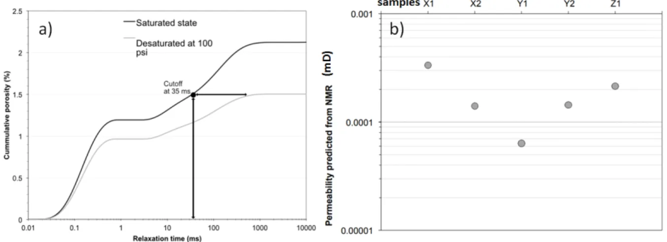
X1 (Figure 12a). The five samples record a T2 cutoff around 30 ± 10 ms, very close to values 625
found in the literature for quartz rich rocks (around 33 ms).
626
627
Figure 12. a) Example of NMR cumulative porosity of sample X1 under saturated and desaturated conditions to
628
measure the T2 cutoff that separates mobile and irreducible water. b) Predicted permeability from NMR in five
629
small core plugs of Grimsel granodiorite using classical parameters from Coates. 630
As formulated in the Coates model (Coates et al., 1991), the NMR predicted
631
permeability is given by:
632
𝑘𝑘 = �Γ𝜙𝜙�4�𝐹𝐹𝐹𝐹𝐹𝐹𝐵𝐵𝑉𝑉𝐹𝐹�2 (14)
633
where Γ is a constant related to pore geometry. Using a standard value for Γ according to the
634
Coates model (Γ=10 when the permeability unit is mD (10-15
m²) and porosity is in %, the
635
five tested plugs have a predicted permeability ranging from 0.14 to 0.35 10-18 m² (average
636
0.20 10-18 m²) except for sample Y1, which has a lower permeability (0.063 10-18 m²)(Figure
637
12b). These values are lower than the average permeability found in the benchmark (see
638
companion paper). However they were obtained at 13 MPa confining pressure whereas the
639
KG2B effective pressure target was 5 MPa. Taking into account the pressure dependence of
640
permeability shown in the companion paper, the NMR predicted permeability values are in
good agreement with the measured permeability range.
642 643
4.6 Permeability Estimation from RC Filter Analog 644
Here we report a new way to analyze the data generated by pore fluid pressure
645
oscillation experiments (see companion paper) based on modeling the rock as a RC filter. The
646
approach has been used by Mckernan et al. (2017) and Rutter and Mecklenburgh (2018). In
647
contrast to the four previous models, this model is based on a physical analog rather than
648
microstructural data. Oscillatory flow of fluid through the pores of a rock is analogous to the
649
flow of electricity through a resistor-capacitor network. A first order resistance-capacitance
650
(RC) filter is shown in Figure 13a. This corresponds to a rock sample (the resistive element)
651
of zero storativity (zero porosity), and the downstream reservoir corresponds to the capacitive
652
element. The transfer function or gain G=Vout/Vin depends on the frequency f because of the 653
time required to charge the capacitor through the resistor. At low frequencies the capacitor is
654
infinitely resistant so a waveform applied as Vin passes unimpeded (provided the output does 655
not draw current). Beyond the break frequency fB the capacitor can conduct so the R and C 656
elements form the arms of a potential divider and the output is progressively attenuated as
657
frequency is increased. This is a low pass filter, because the unattenuated frequencies are low
658
frequencies. The high frequency waveform amplitude attenuation rate (gain) is always 20 dB
659
per decade; it has a slope of -1 on a plot of log G vs log f. The linear prolongation of the high
660
frequency slope intersects the gain = 1 abscissa at a characteristic break frequency (or corner
661
frequency) fB = 1/(2πRC). The output (across the capacitor) of an RC filter also has a 662
particular response to a step change in input voltage, with vout decaying exponentially with 663
time. This was the basis of the widely-used pulse transient decay method proposed by Brace
664
et al. (1968) for the measurement of permeability of tight rocks.
665
666
Figure 13. a) A first order electrical low pass filter analogous to fluid flow through a resistant rock R of zero
667
storage capacity, with a capacitor C analogous to the downstream storage reservoir. Variation of b) phase shift 668
and c) gain A with applied waveform frequency for a low pass electrical filter. 669
670
In addition to progressively attenuating the output waveform, the filter progressively shifts its
671
phase over the frequency range between the two linear segments, from 0° to 90° (Figure 13b).
672
The gain G and phase shift θ can be expressed respectively as:
673 674 𝑮𝑮 =𝑽𝑽𝒐𝒐𝒐𝒐𝒐𝒐 𝑽𝑽𝒊𝒊𝒊𝒊 = 𝟏𝟏 �𝟏𝟏+(𝒇𝒇/𝒇𝒇𝑩𝑩)𝟐𝟐 (15) 675
𝜽𝜽 = − 𝐭𝐭𝐭𝐭𝐭𝐭−𝟏𝟏�𝒇𝒇
𝒇𝒇𝑩𝑩� (16)
676
Higher-order low-pass filters can be formed by cascading first order filters to simulate the
677
behavior of more porous rocks (higher storativity). A rock might be imagined as a series of
678
such filters, with capacitive components corresponding to pore spaces connected by resistors
679
that combine to form the total resistance to flow. Each RC element in series can apply an
680
additional phase shift, but many such phase shifts will result in severe attenuation. Many
681
possible topologies of R and C combinations can be imagined, with the final capacitor
682
corresponding to the downstream volume of the permeameter. Analysis of such combinations
683
is beyond the scope of the present paper. Smaller ratios of rock storativity to downstream
684
storage translate to smaller phase shifts for a given gain, so that the behavior more closely
685
resembles that of a first-order filter.
686
This approach was evaluated on a Grimsel granodiorite sample cut at a high angle to the
687
foliation (called hereafter core C), to investigate how similar its behavior is to that of an RC
688
filter. Pore fluid pressure oscillation tests were conducted with a pressure cycling period
689
ranging from 50 to 12800 seconds (i.e. 7.8 10-5s-1 < f < 2 10-2s-1). Figure 14a shows a plot of
690
log G vs log f for the driving waveform when total confining pressure is 20.0 MPa and pore
691
pressure is 15.5 MPa. As expected the behavior is similar to that of an RC filter with log fB = 692
-2.869 (i.e. fB=1.35 10-3 s-1). The slope in the frequency-dependent region is -1.16, slightly 693
greater than unity, as might be expected for the small degree of storativity (non-zero porosity)
694
within the rock specimen.
695
696
Figure 14. a) Plot of log G versus log f for core C at 4.5 MPa effective pressure and 15.5 MPa pore pressure of
697
argon gas. This is typical of rock behavior as a first order filter with very small storativity in the rock sample 698
(slope of -1.16 close to unity). b) Frequency dependence of permeability calculated for the individual data. The 699
peak in the convex upward curve corresponds to the break frequency. The average of the log k data lying above 700
the break frequency is -18.52. 701
The fluid flow analogs of resistance R and capacitance C are:
702
𝐑𝐑 =𝑳𝑳𝑳𝑳𝑨𝑨𝑨𝑨 and 𝐂𝐂 = 𝜷𝜷𝑫𝑫 (17)
703
where L and A are the length and cross-sectional area of the sample respectively, and βD is 704
the storage of the downstream reservoir (m3/Pa). Permeability can therefore be calculated
705
from the break frequency provided that the frequency-dependence of gain is measured at
706
constant confining pressure and pore pressure conditions:
𝑨𝑨 = 𝟐𝟐𝟐𝟐𝑳𝑳(𝑳𝑳/𝑨𝑨)𝜷𝜷𝑫𝑫𝒇𝒇𝑩𝑩 (17)
708
This yields log k = -18.33 (i.e. k=0.47 10-18 m²) for the tested sample. Leaving aside the most
709
extreme values of very small or very large gain, the average of all the individual permeability
710
measurements is log k = -18.52 ± 0.06 (k=0.30 10-18 m²). The plot of log k vs log f (Figure
711
14b) shows slight upward convexity, similar to what was found for a sandstone by Song and
712
Renner, (2007). One of the KG²B labs (Lab#18, see companion paper) measured a
713
permeability of 0.501 10-18 m² on this sample with the standard approach for analyzing pore
714
pressure oscillation tests (Bernabé et al., 2006), and 0.582 10-18 m² using a transient pulse
715
test.
716 717
5. Complementary Outcome of the Benchmarking Exercise
718
In this section we present additional data produced by the KG²B team in their study of
719
the Grimsel granodiorite core samples. This data set is not as exhaustive as the permeability
720
data set because it was done on a voluntary basis with no specific instructions.
721
5.1. Permeability – Porosity Relationship
722
A log-log plot of permeability vs. porosity (Figure 15) shows a general trend with two
723
outliers and one isolated point aligned with the general cloud consistent with the expected
724
trend of permeability decrease with decreasing porosity. The correlation is not very strong,
725
which is not really surprising as permeability is controlled by the geometrical properties (pore
726
size and shape, topology and connectivity) of the 3D pore or crack network and not simply by
727
the bulk porosity. Nevertheless, a simple power-law can be fitted to the data set (minus two
728
outliers) with an exponent equal to 2 (Figure 15). The sample in the lower left corner was
729
considered as an outlier in the statistical analysis presented in the companion paper: its low
730
permeability can be explained by its porosity being much lower than all the others. A
power-731
law relationship between permeability and porosity has often been invoked (e.g. David et al.,
732
1994 and references therein). Wang et al. (2016) found an exponent between 4 and 5 in their
733
permeability-porosity correlation for two granite gneiss samples. In our KG²B experiments,
734
porosity was measured at room conditions whereas permeability was measured at 5 MPa
735
effective pressure. If both properties were measured under the same pressure conditions, the
736
correlation would probably have been better.