HAL Id: hal-01183878
https://hal.archives-ouvertes.fr/hal-01183878
Submitted on 19 Feb 2016HAL is a multi-disciplinary open access archive for the deposit and dissemination of sci-entific research documents, whether they are pub-lished or not. The documents may come from
L’archive ouverte pluridisciplinaire HAL, est destinée au dépôt et à la diffusion de documents scientifiques de niveau recherche, publiés ou non, émanant des établissements d’enseignement et de
PLR-based heuristic for backup path computation in
MPLS networks
Mohand Yazid Saidi, Bernard Cousin, Jean-Louis Le Roux
To cite this version:
Mohand Yazid Saidi, Bernard Cousin, Jean-Louis Le Roux. PLR-based heuristic for backup path computation in MPLS networks. Computer Networks, Elsevier, 2009, 53 (9), pp.1467 - 1479. �10.1016/j.comnet.2009.01.009�. �hal-01183878�
PLR-based Heuristic for Backup Path Computation
in MPLS Networks
Mohand Yazid SAIDI
aBernard COUSIN
bJean-Louis LE ROUX
c aIRISA/INRIA, Universit´e de Rennes I - Campus de Beaulieu, 35042 Rennes, Francemsaidi@irisa.fr
bIRISA, Universit´e de Rennes I - Campus de Beaulieu, 35042 Rennes, France
bcousin@irisa.fr
cFrance T´el´ecom, 2 Avenue Pierre Marzin, 22300 Lannion, France
jeanlouis.leroux@orange-ftgroup.com
Abstract
To ensure service continuity in networks, local protection pre-configuring the backup paths is preferred to global protection. Under the practical hypothesis of single physical failures in the network, the backup paths which protect against different logical failure risks (node, link and Shared Risk Link Group (SRLG)) cannot be active at the same time. Thus, sharing bandwidth between such backup paths is crucial to increase the bandwidth availability.
In this article, we focus on the optimal on-line distributed computation of the bandwidth-guaranteed backup paths in MPLS networks. As the requests for connection establishment and release arrive dynamically without knowledge of future arrivals, we choose to use the on-line mode to avoid LSP reconfigurations. We also selected a distributed computation to offer scalability and decrease the LSP setup time. Finally, the optimization of bandwidth utilization can be achieved thanks to the flexibility of the path choice offered by MPLS and to the bandwidth sharing.
For a good bandwidth sharing, the Backup Path Computation Entities (BPCEs) require the knowledge and maintenance of a great quantity of bandwidth information (e.g. non aggregated link information or per path information) which is undesirable in distributed environments. To get around this problem, we propose here a PLR (Point of Local Repair)-based heuristic (PLRH) which aggregates and noticeably decreases the size of the band-width information advertised in the network while offering a high bandband-width sharing. PLRH permits an efficient computation of backup paths. It is scalable, easy to be deployed and balances equitably computations on the network nodes.
Simulations show that with the transmission of a small quantity of aggregated informa-tion per link, the ratio of rejected backup paths is low and close to the optimum.
Key words: recovery; local protection; backup LSP; failure risk; SRLG; MPLS;
1 Introduction
The proactive protection of communication becomes increasingly important with the explosion of the number of network real time applications (voice over IP, net-work games, video on demand, etc). Thus, to ensure netnet-work service continuity upon a failure, the proactive protection techniques [1,2] precompute and generally pre-establish backup paths capable to receive and reroute the traffic of the affected primary paths. Two schemes of protection exist: global (end-to-end) and local. With global scheme [1], each primary path is protected by one vertex (or link) disjoint backup path interconnecting the primary source and destination nodes. This pro-tection scheme presents the disadvantage of increasing the recovery cycle [3] since it requires that failure notification reaches the source before the switching from the primary toward the backup path. This last drawback is eliminated with the use of local protection where the recovery is achieved locally and without any control plane notification by the upstream node to the failing component.
With the advent of MPLS [4] in the last decade, the local protection is provided in an efficient manner. In fact, MPLS offers a great flexibility for choosing paths (called Label Switched Paths or LSPs) and thus, the backup paths can be deter-mined so that bandwidth availability is maximized. Two types of backup LSP are defined for MPLS local protection [5]: Next HOP (NHOP) LSP and Next Next HOP (NNHOP) LSP. A NHOP LSP (resp. NNHOP LSP) is a backup path pro-tecting against link failure (resp. node failure); it is setup between a primary node called Point of Local Repair (PLR) and one primary node downstream to the PLR (resp. to the PLR next-hop) called Merge Point (MP). Such backup LSP bypasses the link (resp. the node) downstream to the PLR on the primary LSP. When a link failure (resp. node failure) is detected by a node, this later activates locally all its NHOP and NNHOP (resp. all its NNHOP) backup LSPs by switching traffic from the affected primary LSPs to their backup LSPs.
To ensure enough resource (particularly the bandwidth) after the recovery from a failure, the backup LSPs must reserve the resources they need beforehand. In this way, if we consider that each backup path has its own exclusive resources, the network will be overbooked rapidly since the available resources decrease quickly. Instead and under the practical single failure assumption, resource utilization can be improved by sharing the resources as much as possible between the backup LSPs. For instance, all the backup LSPs protecting against different failure risks (a risk is formed of the network components which can fail simultaneously) can share their resource allocation on their common links. Indeed, such backup paths cannot use their resources simultaneously since they cannot be active at the same time (there is at most one failure occurrence at any time).
To increase the number of LSPs that can be setup in a network (i.e. to decrease the blocking probability), the resource sharing should be taken into account when
the backup LSPs are computed. Three functionalities are necessary to perform such computations in a distributed environment: information collection, information dis-tribution and path determination. The first functionally gathers the structures and properties of the backup LSPs setup in the network. In practice, each network node stores the path links, the bandwidth and the risks protected by the backup LSPs traversing it. Such information can be obtained easily and without any additional overhead when the backup LSPs are signaled as in [5]. The second functionality reorganizes and transmits the collected information to nodes supporting the BPCEs (Backup Path Computation Entity). We note that for a same capability of bandwidth sharing, less the size of the transmitted information is, better the functionality of distribution is. Finally, the last functionality searches for the backup LSPs provid-ing the desired protection and verifyprovid-ing the bandwidth constraints.
In this article, we focus on the mechanisms allowing an efficient distribution of the bandwidth information and enabling the bandwidth guaranteed-backup LSP com-putation to be performed on-line and locally by the PLRs. Hence, we propose a new PLR-based heuristic (PLRH) aggregating and reducing significantly the size of the bandwidth information advertised in the network. With our heuristic, the backup LSPs are computed and configured by the same nodes which correspond to the backup LSP PLRs. This eliminates the communication between the entities com-puting the backup LSPs (BPCEs) and those configuring the backup LSPs (PLRs). Besides, PLRH is scalable (balances the computations fairly on the network nodes), shares effectively bandwidth between the backup LSPs and is capable to compute backup LSPs protecting against the three types of failure: node, link and Shared Link Risk Group (SRLG) [6].
The rest of this article is organized as follows: section 2 describes the three types of failure risks which gather network components in entities failing simultaneously. With the adoption of the single physical failure hypothesis, we give the formulas allowing the computation of the minimal protection bandwidth to be reserved on each unidirectional link. In section 3, we review some works related to the band-width sharing. Then, we explain in section 4 the principles of PLRH. At the end of this section, we describe slight extensions to be introduced in the IGP (Interior Gateway Protocol) protocols in order to deploy PLRH. In section 5, we present simulation results and analysis. The next section is dedicated to the conclusions. Finally, in the last section (annex), we study the impact of the network size and the protection locality on the volume of the information that should be advertised in the network, for the PLRH deployment.
2 Failure risks and bandwidth sharing
To deal with any single physical failure in a logical (MPLS) layer, three types of (logical) failure risks are defined: link, node and SRLG. The first type of failure risk
Fig. 1. Topology correspondence
corresponds to the risk of a logical link failure due to the breakdown of an exclusive physical component of the logical link. The second type of failure risk corresponds to the risk of a logical node failure due to the breakdown of an exclusive physical component of the logical node. Finally, the third type of risk corresponds to failure risk of a common physical component (optical fiber, crossconnect, etc) shared by a group of logical links [6].
In figure 1, two topologies corresponding to the same network are depicted. The first one (figure 1 (a)) is obtained according to the Data Link neighbourhood infor-mation; the second one (figure 1 (b)) is determined with the use of only the (IP) Network neighbourhood information. As we see, the optical crossconnect OXC in figure 1 (a) is not visible by the IP (and MPLS) layer. This crossconnect is an op-tical component used to connect router E to routers B and D. Hence, the network link E-B (resp. link E-D) in figure 1 (b) corresponds to the optical path E-OXC-B (resp. optical path E-OXC-D) in figure 1 (a). As a result, the two IP (MPLS) links
E-B and E-D should be gathered in one SRLG risk1 to cope with the failure of the
crossconnect OXC. Similarly, to protect against the failure of a physical link A-B (resp. physical node A) for instance in MPLS layer, one (MPLS) failure risk A-B (resp. A) of type link (resp. node) must be defined.
In order to ensure enough bandwidth upon a failure, minimal quantities of band-width must be reserved on links. To determine such quantities, [9] defines two con-cepts: the protection failure risk group (PFRG) and the protection cost. The PFRG of a given arc λ, noted PFRG (λ), corresponds to a set which includes all the risks protected by the backup LSPs traversing the arc λ. The protection cost of a risk r on an arc λ, noted δλ
r, is defined as the cumulative bandwidth of the backup LSPs
which will be activated on the arc λ upon a failure of the risk r. For a SRLG risk
srlg composed of links (l1, l2, .., ln), the protection cost on an arc λ is determined
as follows: δλ srlg = X 0<i≤n δλ li (1)
To cope with any single failure, a minimal quantity of protection bandwidth Gλ
must be reserved on the arc λ. Such quantity Gλis determined as the maximum of
1 We note that the IGP-TE protocols (OSPF-TE [7] and ISIS-TE [8]) are extended to
Fig. 2. Bandwidth allocation on an arc λ
the protection costs on the arc λ.
Gλ = Maxr∈P F RG(λ)δrλ (2)
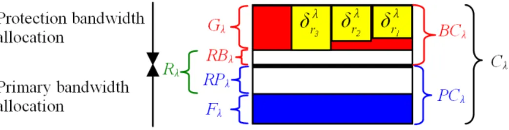
In order to control and specify the quantity of bandwidth dedicated for protection and to separate the task of primary LSP computation from that of backup LSP com-putation, the bandwidth capacity Cλ on arc λ can be divided in two pools: primary
bandwidth pool and protection bandwidth pool (figure 2). The primary bandwidth pool on an arc λ has a capacity P Cλ and it is used to allocate bandwidth for
pri-mary LSPs. The protection bandwidth pool on an arc λ has a capacity BCλ and it
is used to allocate bandwidth for backup LSPs. We note that the separation of the bandwidth in two pools is not necessary to apply all the backup LSP computation techniques described in this article (except that described in [10]). It is adopted here to limit the amount of bandwidth used for protection and thus increase the bandwidth sharing.
To ensure the respect of bandwidth constraints upon a failure, the minimal protec-tion bandwidth reserved on each arc λ must verify:
Gλ ≤ BCλ (3)
To keep (3) valid after the setup of a backup LSP b of bandwidth bw (b) and pro-tecting against the risks in FR (b) (FR (b) is a set composed of all the risks whose failure activates the backup path b), only the arcs λ verifying the following inequal-ity can be selected to be in the LSP b:
Maxr∈F R(b)δrλ ≤ BCλ − bw(b) (4)
Finally, we define the residual protection bandwidth RBλ as the amount of
RBλ = BCλ − Gλ (5)
3 Related Work
Recently, a great deal of work is addressing the path protection in order to find algorithms and mechanisms allowing on-line computation of the optimized backup paths. Several solutions are then proposed but a large number of them, like [11] and [12], deals only with failure risks of type link or node.
In this section, we will be more interested on computation techniques (especially, on bandwidth information distribution methods) of bandwidth-guaranteed backup LSPs which deal with all the types of failure risks (SRLG, link and node). Ac-cording to the computation environment, we distinguish two types of techniques: centralized and distributed.
In a centralized environment, the server can memorize all the information (topol-ogy, structures and properties of all the backup paths) necessary to compute the optimized backup paths. Such information is obtained from the IGP protocols and from the paths computed by the server itself. Obviously, with complete information knowledge, the bandwidth sharing capabilities can be exploited efficiently to com-pute the optimized backup paths. For instance, [13] uses an ILP (Integer Linear Programming) formulation to compute a primary path and its backup path (with the use of the end-to-end protection) so that the additional bandwidth they need is minimal. Although the high-quality of bandwidth sharing obtained with centralized servers, their utilization can increases significantly the LSP setup time after the oc-currence of a failure and present some well known disadvantages like the formation of bottlenecks around the server and the sensitivity to the failure or overload of the server.
Instead and to avoid long LSP setup time upon a failure, distributed techniques are preferred to centralized techniques. As the quality of the distributed techniques computing the backup paths depends closely on the algorithms implementing the functionality of information distribution (cf. section 1), we will focus below on the study of these algorithms; for path computation, various variants of the Dijkstra’s algorithm or ILP formulation can be applied.
In a first obvious solution [14], Kini proposes to flood within the IGP-TE (Inte-rior Gateway Protocol Traffic Engineering) protocols the topology information, the primary bandwidth, the capacities and all the protection costs of the risks on the topology arcs in the network. In this way, each node has a complete knowledge of the information necessary to the backup LSP computation and as a result, it can use a similar model as in the centralized environment to perform the computations. This computation technique increases the bandwidth availability but it overloads
the network with large and frequent messages advertising the protection costs (the number of protection costs advertised for an arc maybe large and up to the number of failure risks in the network). Another similar solution for backup LSP computa-tion is proposed in [9]. To decrease the size of messages advertising the bandwidth information, [9] suggests to flood within IGP-TE protocols the structures and prop-erties of the backup LSPs. To reduce the advertisement frequency, [9] recommends the use of the facility backup protection (described in [5]). Like the first compu-tation technique, this second technique floods the network with the transmission of a large quantity of information advertising the structures and properties of the backup LSPs. To scale well, [10] proposed the PCE-based MPLS-TE fast reroute technique in which no control message is necessary to compute the bandwidth-guaranteed backup LSPs. With this technique, a separate PCE (path computation element) is associated with each failure risk in order to compute the backup LSPs which will be activated at the failure of that risk. This computation technique is ef-ficient when there are no SRLGs in the network. Otherwise, the PCE-based MPLS-TE fast reroute technique requires a mechanism distinguishing a node failure from a link failure (as [15]). This increases significantly the recovery cycle of all the communications. In addition, the PCE-based MPLS-TE fast reroute technique re-quires that non disjoint SRLGs be managed by a same PCE. This centralizes the path computations and introduces same problems as that encountered in the cen-tralized environments. To get around the drawbacks of the PCE-based MPLS-TE fast reroute technique, [16] proposed to share the protection costs of each SRLG between all the end nodes of that SRLG. This last backup LSP computation tech-nique balances equitably the computations on the network nodes but it introduces a new drawback which consists in the size increase of the control messages.
To offer scalability without increasing the recovery cycle, new computation heuris-tics which approximate and reduce the bandwidth information (protection costs especially) transmitted in the network have emerged. Hence, once the bandwidth information is collected, nodes aggregate it before its flooding in the network.
In a first computation heuristic (residual bandwidth-based heuristic) presented in [14], Kini proposes to approximate the protection cost δλ
r of a risk r on a
(uni-directional) link λ by the maximum of protection costs (Maxr(δrλ)) on that link.
In this way, only one aggregated value per link is advertised in the network. This heuristic has the advantage of facility of its deployment. Indeed, this requires only slight modifications to IGP-TE protocols [7,8] for the advertisement of the minimal quantities of protection bandwidth on links. However, this heuristic does not exploit efficiently the bandwidth sharing. As a result, the number of backup LSPs that can be built with this heuristic is low (i.e. the blocking probability is high). In order to improve the bandwidth sharing and resource availability, the previous heuristic can be enhanced to better estimate the protection costs. Hence, with the improved heuristic of Kini (IKH), the protection cost δλ
r is approximated by the minimum
be-tween the highest protection cost Maxr(δrλ) on the arc λ and the primary bandwidth Frreserved on the risk r. In practice, this last heuristic has performances
compara-Fig. 3. Protection pool of an arc λ
ble to those of the residual bandwidth-based heuristic since the primary bandwidth
Frreserved on the risk r (case of a node) is often greater than the highest protection
cost Maxr(δλr) on the arc λ.
4 PLR-based backup path computation heuristic (PLRH)
For simplicity, we consider here that the capacity Cλ of each arc λ is divided in two
disjoint pools (protection pool and primary pool), as in figure 2. In this manner, the task which computes the backup LSPs can be independent from that determining the primary LSPs.
4.1 PLRH principles
The PLRH allows an efficient approximation of the protection costs on the links with the advertisement of a small quantity of aggregated protection bandwidth in-formation. It is based on the two following principles:
• An arc λ can be used to establish a new backup LSP b requiring a quantity of
bandwidth bw (b) if and only if the protection costs of the risks protected by such LSP (on λ) are lower or equal to BCλ- bw (b). As a result, the knowledge of the
partial information consisting of the protection costs (and their corresponding risks) which are higher than BCλ- bw (b) is sufficient to decide without mistake
if λ can be selected to be in the backup LSP b.
• Some values of protection cost on an arc can be very low. Aggregate and
approx-imate these values by their maximum can decrease the quantity of protection in-formation to be advertised in the network with slight or without the deterioration of the bandwidth sharing.
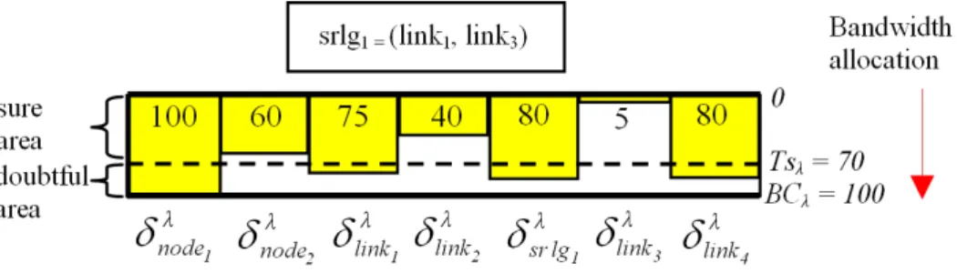
To show how the PLRH exploits the two above principles, let us consider an ex-ample. In figure 3, the protection pool of an arc λ is illustrated. This protection pool has a capacity BCλ of 100 units. It was used to allocate the bandwidth for
Algorithm 1 Simplified algorithm run by the outgoing node oλ of an arc λ parameters:
Bandwidth: T sλ; {threshold}
Integer: xλ; {maximal size of the xλ vector}
inputs:
const Risk id: generic risk ← “-” ;
Sorted list<RISK id, Bandwidth>: costsλ; {protection costs (and their correspond-ing risk identifiers), on the arc λ, sorted accordcorrespond-ing to the decreascorrespond-ing values of protection cost}
variables:
Sorted list<RISK id, Bandwidth>: old xλ vector, new xλ vector ; begin algorithm
old xλ vector ← empty vector () ;
while true do
wait (costsλ) ; {wait for a change in the sorted list costsλ}
new xλ vector ← costsλ.elements at (1, xλ) ; {Assign to the new xλ vector, the xλhighest protection costs and their corresponding risk identifiers}
if costsλ.element at (xλ + 1) > T sλthen
new xλ vector.element at (xλ).setRiskId () ← generic risk ; {Replace, in
new xλ vector, the identifier corresponding to the xthhighest protection cost by the special identifier generic risk}
end if
if old xλ vector 6= new xλ vector then
advertise (λ, new xλ vector) ;
old xλ vector ← new xλ vector
end if end while end algorithm
node1, node2, link1, link2, link3, link4 and srlg1. The protection costs associated
to these risks are as follows:
δλ node1 = 100, δ λ node2 = 60, δ λ link1 = 75, δ λ link2 = 40, δ λ link3 = 5, δ λ srlg1 = 80, δλ link4 = 80.
When the maximal quantity of bandwidth maxbw2that a LSP can claim is known
(in figure 3, maxbwis equal to 30), the application of Principle 1 permits to deduce
that all the risks whose protection costs are lower or equal to the threshold T sλ
(T sλ = BCλ− maxbw) can be ignored (approximated by zero) when a new backup
LSP is computed. In fact, the selection of the arc λ to be in a new backup LSP b of bandwidth bw (b) cannot lead to the violation of bandwidth constraints upon a failure of a risk r if the protection cost δλ
r is lower or equal to the threshold T sλ.
2 When max
bwis not known, we can set its value on a link λ to BCλ(worst case). More-over, we note that we can process a protection request claiming a quantity of bandwidth which is higher than maxbwby splitting it in two or more requests of bandwidth lower than
Algorithm 2 Simplified algorithm run by each node receiving a xλ vector inputs:
const Risk id: generic risk ← “-” ;
Array (Risk id × Arc)→ Bandwidth: costs ; {risk costs on all the network arcs} variables:
Sorted list<RISK id, Bandwidth>: xλ vector ; Bandwidth: min cost ;
Arc: λ ; begin algorithm
(λ, xλ vector) ← receive () ; {receives an advertised message and returns the values of
the arc λ and the xλ vector included in this message}
if xλ vector.element at (xλ vector.getSize ()).getRiskId () 6= generic risk then
min cost ← 0 ;
else
min cost ← xλ vector.element at (xλ vector.getSize ()).getCost () ; end if
for all (Risk id: a risk) do
cost [λ, a risk] ← min cost ;
end for
for all (Integer: i ∈ [1, size]) do
costs [λ, xλ vector.element at (i).getRiskId ()]
← xλ vector.element at (i).getCost () ;
end for end algorithm
This results from the following inequalities:
δλ r ≤ T sλ = BCλ− maxbw bw(b) − maxbw ≤ 0 ⇒ δλ r + bw(b) ≤ BCλ
Obviously, the elimination of the protection costs, which are lower or equal to the threshold T sλ (T sλ = BCλ− maxbw = 70) from the information to be advertised
in the network, does not alter the decision of excluding (or including) the arc λ in a next backup LSP computation. Typically, in figure 3, the outgoing node oλto the
arc λ, which is responsible3 of the advertisement of the protection costs {δλ r}r on
the arc λ, approximates the protection costs of node2, link2and link3 by zero. As a
result, these risks (node2, link2and link3) and their corresponding protection costs
on the arc λ are not advertised in the network.
When the value maxbwis high (or ignored by the nodes of the network), the
quan-tity of bandwidth information advertised for each arc of the network topology can
3 The end nodes of an arc λ know all the risks (and their associated protection costs on that
arc λ) using λ for protection. This information can be obtained, without overhead, when the backup LSPs are signaled.
be high and unacceptable. To avoid the flooding of the network while maintaining bandwidth sharing high, PLRH limits the size of the protection bandwidth infor-mation that is advertised for each arc λ to a vector (called xλ vector) composed
of xλ elements. Each xλ vector component includes a couple of protection cost
and its associated risk. Besides, the costs conveyed in the xλ vector of an arc λ
correspond to the xλ highest values of protection cost. In this manner, each node
receiving a xλ vector of an arc λ deduces the xλhighest protection costs (and their
corresponding risks) on the arc λ and approximates all the rest of protection costs by the (xλ)th highest protection cost (principle 2 of PLRH) on the arc λ. For
in-stance, if we consider that xλ is equal to 2 in figure 3, the outgoing node oλ to the
arc λ will send the following xλ vector: [(node1, 100), (generic risk, 80)] (where
generic risk refers to any risk different from those conveyed in the xλ vector).
4.2 PLRH algorithm description
With the combination of the PLRH principles 1 and 2, we construct the algorithms Alg. 1 and Alg. 2 which specify the steps of the protection cost advertisement and collection. Thus, Alg. 1 describes the procedure of protection cost advertisement which limits the transmitted bandwidth information for each arc λ, to a xλ vector.
This vector contains, at most, the xλhighest protection costs which are greater than
the threshold T sλ. Concerning Alg. 2, it specifies the procedures used to
approxi-mate the protection costs from the received xλ vector information.
In order to increase the bandwidth sharing and to reduce the size of messages trans-mitting the xλ vectors, each node running Alg. 1, eliminates from its protection
cost table all the entries corresponding to the risks which are included in others. In figure 3 for instance, the SRLG risk srlg1 is made of two link risks: link1 and
link3. As a result, these two risks (link1and link3) and their corresponding
protec-tion costs are deleted from all the protecprotec-tion cost tables before any advertisement of the xλ vectors. After this step, the outgoing node oλto each arc λ builds a list costλ
containing all the risks and their protection costs on λ. This list is then sorted ac-cording to the decreasing values of the protection cost. For the example in figure 3, the sorted list costλ is as follows: [(node1, 100), (srlg1, 80), (link4, 80), (node2,
60), (link2, 40)].
At each change in the sorted list costλ, node oλruns the following instructions (cf.
Alg. 1): oλ extracts from the list costλ the first xλ couples conveying the
protec-tion costs which are greater than the threshold T sλ (xλ and T sλ are parameters of
Alg. 1). Then, oλ checks if there is a change in the value of the xλ vector. If so, it
advertises the new xλ vector, else it does nothing.
When a node (different from the end nodes of λ) receives a xλ vector
costs on the arc λ.
According to the threshold value (T sλ) and to the (xλ + 1)th highest protection
cost (denoted by xλ plus 1 cost) on an arc λ, the PLRH decision of excluding the
arc λ in the next backup LSP computation can be “sure and correct” or “possibly wrong”. Two areas are defined to measure the correctness degree of the protection cost approximation used by PLRH: doubtful area (xλ plus 1 cost > T sλ) and sure area (xλ plus 1 cost ≤ T sλ).
4.2.1 Doubtful area (xλ plus 1 cost > T sλ)
When the (xλ + 1)th highest protection cost on an arc λ is in the doubtful area,
the advertisement of a xλ vector of a maximal size xλ can be insufficient to decide
without mistake if the arc λ can be selected to be in a new backup LSP.
In figure 3 for instance, the (xλ + 1)thhighest protection cost on the arc λ is in the
doubtful area if xλ ≤ 2. Thus, the advertisement of a xλ vector containing at most
the two highest protection costs on λ can be insufficient. Typically, with xλ = 2,
the outgoing node oλ to the arc λ transmits a xλ vector including (at most) the
two highest protection costs which are greater than the threshold T sλ = 70. This xλ vector is deduced from the sorted list costsλ and corresponds to: [(node1, 100),
(generic risk, 80)] (Alg. 1). We note that the last couple of the xλ vector sent by
the node oλ contains a special risk, called generic risk, to indicate that the (xλ + 1)thhighest protection cost on the arc λ is in the doubtful area.
When a node plr receives the xλ vector transmitted by oλ, it updates its protection
cost table by approximating the protection costs on the arc λ as follows (Alg. 2):
δλ node1 = 100 ∀r(r is a risk ∧ r 6= node1) : δrλ = 80
As we see here, all the risks whose protection costs on the arc λ are not transmit-ted within the xλ vector, are aggregated and approximated by the (xλ)th highest
protection cost on this arc. As this last cost is higher than the threshold, any com-putation of a new backup LSP b, protecting against a risk which is not conveyed in the transmitted xλ vector of λ and claiming a quantity of bandwidth bw (b)
(bw (b) > BCλ − xλ plus 1 cost), excludes by mistake the arc λ. However, any
other computation will include or exclude the arc λ without mistake.
In figure 3 for instance, after the reception by node plr of this xλ vector (xλ vector
= [(node1, 100), (generic risk, 80)]), node plr excludes by mistake the arc λ in its
next computation of a backup LSP if this last one claims a quantity of bandwidth greater than 20 (20 = BCλ − 80) and protects against failure risks which do not
belong to {node1, srlg1, link4}; otherwise, the arc λ is included or excluded
with-out mistake.
Example: Consider the example depicted in figure 3 and assume that:
• The bandwidth quantities desired by new backup LSPs are uniformly distributed
in the interval [1, 30].
• Any backup LSP is dedicated to the protection of only one failure risk.
• The risk to be protected by a new backup LSP is randomly (uniformly) chosen
among the set of failure risks FR.
• The last xλ vector advertised by the node oλ for the arc λ is [(node1, 100),
(generic risk, 80)]).
The probability to reject the arc λ by mistake in a next backup LSP computation is determined as follows:
Prej/m (λ) = ( 30 - (100 - 80) ) * [ (card (FR) - card ({node1, srlg1, link4}) ] / [
(30 -1 + 1) * (card (FR) ] = [(card (FR) - 3] / (3 * card (FR)).
For the minimal number of risks where (card (FR) = 7), we have Prej/m(λ) = 19%.
For the maximal number of risks where (card (FR) = ∞), we have Prej/m (λ) = 33,33%.
4.2.2 Sure area (xλ plus 1 cost ≤ T sλ)
When the (xλ + 1)th highest protection cost on an arc λ is in the sure area, the
advertisement of a xλ vector of a maximal size xλ is sufficient to decide without
mistake if the arc λ can be selected (or not) to be in a new backup LSP (Principle 1 of PLRH).
In figure 3 for instance, the (xλ + 1)thhighest protection cost on the arc λ is in the
sure area when xλ > 2. Thus, the advertisement of a xλ vector containing at least
the three highest protection costs on λ is sufficient. Typically, with the choosing of
xλ equal to 3, the outgoing node oλ to the arc λ transmits a xλ vector including
(at most) the three highest protection costs which are greater than the threshold
T sλ = 70. This xλ vector is deduced from the sorted list costsλ (Alg. 1) and
corresponds to: [(node1, 100), (srlg1, 80), (link4, 80)].
When a node plr receives the xλ vector transmitted by oλ, it updates its protection
cost table by approximating the protection costs on the arc λ as follows (Alg. 2):
δλ node1 = 100 ∧ δ λ srlg1 = 80 ∧ δ λ link4 = 80
∀r(r is a risk ∧ r 6= node1∧ r 6= srlg1∧ r 6= link4) : δλr = 0
Contrarily to the case xλ plus 1 cost > T sλ where the protection costs of the
risks, which are not conveyed in the advertised xλ vector, are approximated by the
are aggregated and approximated by zero. As explained in the previous section, this approximation does not alter the decision of including or excluding the arc
λ in the next computation of a backup LSP b. Indeed, if the new backup LSP b
protects against the failure of a risk belonging to the set {node1, srlg1, link4},
node plr can deduce easily the exact value of the highest protection cost on λ of the risks protected by b. This highest protection cost corresponds to 100 units if
b protects against the failure of node1, 80 units otherwise. As a result, node plr
decides without mistake if the arc λ can be selected to be in b or not (formula (4) in section 2). When the new backup LSP b is planned to protect against the failure risks which do not belong to the set {node1, srlg1, link4}, node plr selects the arc
λ, without risk of mistake, when it computes the backup LSP b (cf. Principle 1 of
PLRH in section 4.1).
At this point, we deduce that with the advertisement of partial information about the protection costs (xλ vectors of a limited size), the decision of including or
excluding an arc in a backup LSP computation can be done with high degree of correctness. It results that PLRH scales well since the transmission frequency and the size of messages advertising the protection bandwidth information can be re-duced significantly without the deterioration of the bandwidth sharing possibilities. Indeed, the size decreases since at most the xλ highest protection costs (and their
corresponding risks) are transmitted in the network, for each arc λ. Moreover, the
xλ vector transmitted for an arc λ does not change at each establishment of a new
backup LSP passing through the arc λ. This decreases also the frequency of adver-tisements since it is not necessary to flood a xλ vector as long as it is unchanged.
Finally, we note that we can obtain same performances as with complete infor-mation knowledge when the parameters {xλ}λ are infinite. In such case, only the
protection costs which are greater than the threshold on an arc are advertised. An-other approach enhancing the quality of the protection cost approximation used in PLRH can consists to regulate the value of xλ according to the load of the arc λ
(i.e. a high value of xλis assigned to the arc λ when the number of protection costs
on λ which are greater than the threshold T sλ is high).
4.3 IGP-TE extensions to support PLRH
Another important advantage of PLRH is its easiness of deployment in MPLS net-works. Concretely, slight extensions to the IGP-TE protocols are sufficient to per-mit the distributed computation of backup LSPs protecting against the three types of risk: link, node and SRLG.
Hence, to advertise the protection bandwidth information (i.e. the xλ vectors), we
propose to use and extend the TE parameters defined in [7] (for OSPF-TE) and [8] (for ISIS-TE). A new sub-TLV field (transmitted within the LSA field for OSPF
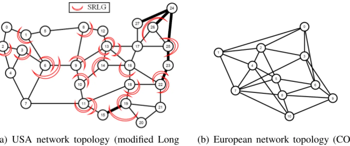
(a) USA network topology (modified Long Haul topology including SRLGs)
(b) European network topology (COST 239)
Fig. 4. Test networks
and within the LSPDU field for ISIS) is then defined and associated to each arc. This field transports for each arc λ its corresponding xλ vector.
5 ANALYSIS AND SIMULATION RESULTS
5.1 Simulation model
We evaluated the performance of our proposed heuristic PLRH by comparing it to the Kini’s flooding-based algorithm (FBA) and to the Kini’s heuristic (IKH) de-scribed in section 3. Our choice is motivated by the following reasons:
• With FBA, all the protection costs are advertised in the network. In this way,
the backup LSPs are computed in an efficient manner, without any bandwidth waste (due to approximations). Although, this algorithm is not practical (i.e. it floods the network), we used it in our simulation to measure the quality of the approximation provided by our heuristic. We note that FBA corresponds to a particular case of PLRH (null thresholds and infinite size of xλ vectors on all
the network arcs).
• With IKH, the number and size of messages advertising the protection costs are
decreased significantly. This heuristic uses only the maximal cost on a link for backup LSP computation and as a result, a (large) amount of bandwidth could be wasted on links. Contrarily to FBA, IKH is practical and it was used in several backup LSP computation algorithms (like in [11,13]).
In our simulation, we chose to divide the total available bandwidth of each arc into two pools (protection pool and primary pool). In this way, our measurements are not distorted by external parameters due to the task of primary LSP computation.
At each arrival of a request asking for a backup LSP computation, PLRH and IKH use their approximation model to compute the protection costs. Then, they check for validity of the inequality (4) and decide if the arc can be selected or not in the next backup LSP computation.
5.1.1 Topologies, SRLGs and traffic matrix generation
Our simulations use two well known network topologies. The first one [17,18], which is a USA network (it is the Long Haul network topology modified to include SRLGs), is depicted in figure 4(a) and is composed of 28 nodes, 45 bidirectional links and 22 SRLGs. It is a network topology of a large size where the average degree of nodes is equal to 3.21. To take SRLG failures into account, we added to the topology a large number of SRLGs (22 SRLGs). We note that these SRLGs are generated so that (1) they verify the geographical neighbourhood property4
(see figure 1) and (2) the protection against any failure risk remains physically possible. The second network topology, corresponding to an European network [18,19] (it is the COST 239 network topology) that is depicted in figure 4(b), is composed of 11 nodes and 26 bidirectional links. It is a network topology of a small size where the average degree of nodes is high and equal to 4.73. To study the performances of PLRH in networks without SRLGs, we do not add any SRLG to the European network. Another network topology with different characteristics (50 nodes, 87 bidirectional links and 25 SRLGs) is used in our simulations. It can be found in [20].
The traffic matrix is generated randomly and consists of requests arriving one by one and asking for quantities of bandwidth uniformly distributed between 1 and 10 units. The head-end and tail-end routers of each primary LSP are chosen ran-domly among the network routers.
5.1.2 Primary and backup path computations
To focus only on the performance impact of the compared methods on the backup path computation, we have separated the task of primary path computation from that computing the backup paths (i.e. the task computing the primary LSPs is in-dependent from that computing the backup LSPs). Thus, we divided the capacity of each unidirectional link in two disjoint pools: primary pool and protection pool. The primary pool is used to allocate the bandwidth for the primary LSPs whereas the protection pool is used for backup LSP bandwidth allocations.
In our simulations, we considered that the primary pool capacities are sufficient to satisfy all the establishment requests of primary LSPs. In this manner, the same
4 Since a SRLG is composed of logical links that share a common physical component,
primary LSPs, which are computed according to the shortest path first algorithm (SPF with unitary weights), are used to compare PLRH to FBA and IKH.
All the protection pool capacities of the network links in figure 4 are equal to 100 units except the bold links in figure 4(a) which have a capacity of 300 units. The backup LSPs are computed according to the constrained shortest path first al-gorithm (CSPF with unitary weights). Concretely, the LSPs correspond to shortest paths verifying the bandwidth constraints and bypassing the protected risks.
5.1.3 PLRH variants
Four variants of PLRH are used in our simulations. The first one P LRH(∞,90)uses
a high threshold (T sλ = 90 on light links and T sλ = 290 on bold links) and xλ vectors of an infinite size (∀λ : xλ = ∞) on all the arcs. The second variant P LRH(2,0) uses xλ vectors of a maximal size equal to 2 (∀λ : xλ = 2) but it
does not employ the threshold (∀λ : T sλ = 0). The third variant P LRH(5,0) uses
xλ vectors of a maximal size equal to 5 (∀λ : xλ = 5) and a null threshold (∀λ : T sλ = 0). Finally, the last variant P LRH(5,90) uses a high threshold (T sλ = 90 on
light links and T sλ = 290 on bold links) and xλ vectors of a maximal size equal
to 5 (∀λ : xλ = 5). We note that the variants P LRH(2,0) and P LRH(5,0)are useful
when we do not have any information about the maximum quantity of bandwidth that a LSP can claim. Otherwise, the two other variants are more practical since they decrease the frequency of xλ vector advertisements.
5.2 Comparison metrics
Four metrics are used for the comparison of PLRH to FBA and IKH: ratio of re-jected backup LSPs (RRL), average protection bandwidth parameter changes (APC), protection bandwidth utilization (PBU) and highest protection cost average (HCA).
The first metric measures the ratio of backup LSPs that are rejected because of the lack of protection bandwidth. This metric is computed as the ratio between the number of backup LSP requests that are rejected and the total number of backup LSP requests.
The second metric measures the (average) rate of changes of the bandwidth protec-tion parameters, used to approximate the different protecprotec-tion costs. It is computed as the ratio between the number of changes in the bandwidth protection parame-ters and the number of satisfied backup LSP computation requests. For PLRH, each change in the xλ vectors increases APC whereas only the changes of the highest
protection costs on arcs are counted with IKH. We note that higher the APC value is, larger the advertisement frequency of messages conveying the protection band-width information is.
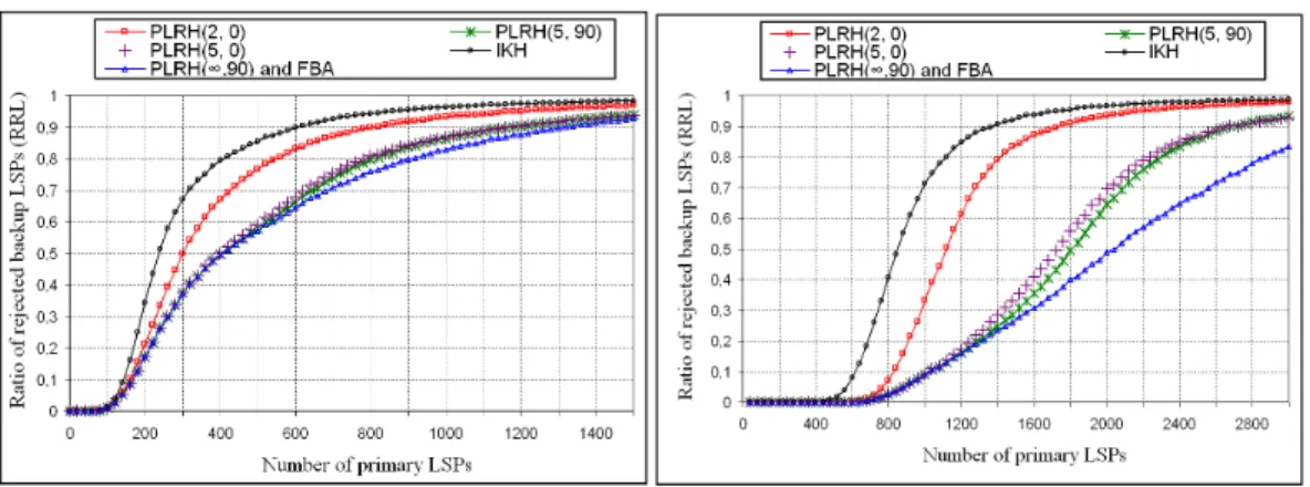
(a) USA network topology (b) European network topology Fig. 5. Ratio of rejected backup LSPs (RRL)
The third metric measures the efficiency of bandwidth sharing. It is computed as the ratio between the sum of the cumulated bandwidth of backup LSPs on arcs and the sum of all the protection capacities. Formally, it is determined as follows:
P BU =P(λ, l) \ l is a link riskδλ l/
P
λBCλ.
The last metric measures the average rate of bandwidth which is really used for protection (note that the bandwidth used for protection is equal to the highest protection cost on each arc). It is computed as the ratio between the sum of the highest protection costs on arcs and the sum of all the protection capacities (i.e.
HCA =PλMaxr(δrλ) /
P
λBCλ).
At each establishment of 20 primary LSPs, the four metrics RRL, APC, PBU and
HCA are computed for each backup LSP computation technique (FBA, IKH and PLRH). We point out that our simulation results correspond to the average values
of 1000 runs generated randomly with different seed values.
5.3 Results and analysis
Figure 5 depicts the evolution of RRL as a function of the number of primary LSPs established in the network. As expected, the various variants of PLRH have RRL values better and lower than those of IKH. This is due to the protection bandwidth information advertised with PLRH which includes that transmitted with IKH. In-deed, the unique protection cost Maxr(δλr) transmitted for each arc λ with IKH is
always included in the first couple of the xλ vector advertised with PLRH.
We also observe in figure 5(a) (resp. in figure 5(b)) that for the 100 (resp. 500) first primary LSPs, the RRL of PLRH and IKH are very similar and close to zero. This is due to the very small quantities of protection bandwidth, generally lower than the threshold, allocated on the network topology arcs (see figure 8). As a result, almost all the arcs are selected and participate to the computation of the backup LSPs
protecting the 100 (resp. 500) first primary LSPs in figure 5(a) (resp. in figure 5(b)).
After the establishment of the 100 (resp. 500) first primary LSPs in figure 5(a) (in figure 5(b)), the RRL of IKH increases more quickly than those of the PLRH variants since the quality of protection cost approximation used in PLRH is better than that of IKH. Whereas IKH approximates all the protection costs on an arc (λ) by the highest cost Maxr(δλr), PLRH approximates them by a protection cost
which is lower than Maxr(δrλ).
With regard to FBA and to the four variants of PLRH used in our simulations, figure 5 shows that the RRL values of P LRH(2,0) are very higher than those of
P LRH(∞,90) and FBA. This means that the advertisement of only two protection
costs per arc is not sufficient to get a RRL close to that obtained with the complete knowledge of the protection bandwidth information (P LRH(∞,90) and FBA). We
observe also in figure 5(a) (resp. in figure 5(b)), especially for the 600 (resp. 1300) first primary LSPs, that the RRL values of P LRH(5,0), P LRH(5,90), P LRH(∞,90)
and FBA are very similar. Thus, the transmission of the five highest protection costs (and their corresponding risks) seems sufficient to obtain a high-quality protection cost approximation. This can be explained by (1) the locality of the PLRH heuristic (cf. annex) and (2) the heterogeneity of protection costs on arcs (due to the het-erogeneity of backup LSPs). In fact, the locality of the backup LSP computation guarantees that the number of high protection costs (typically, the protection costs which are higher than the threshold) is limited and depends on the neighbourhood of the risks to be protected whereas the heterogeneity of protection costs on an arc results in a significative difference between the xth highest protection costs and
their corresponding protection capacities (higher the difference is, better the pro-tection cost approximation is). In our simulation scenario for instance, we observe for the same value of xλ (xλ = 2 or xλ = 5), the protection cost approximation
quality of PLRH on the USA network topology is better that obtained on the Euro-pean network topology. This comes from the average node degree of the EuroEuro-pean network topology which is higher than that of the USA network topology (i.e. the
(a) USA network topology (b) European network topology Fig. 6. Average protection bandwidth parameter changes (APC)
close neighbourhood area in the European network is larger than that corresponding to the USA network).
Concerning the second metric, figure 6 shows that FBA has higher APC values than those of PLRH and IKH. This can be explained by the systematical advertisement of protection costs used with FBA. In fact, at each establishment of a new backup LSP, FBA advertises the new values of protection costs (of the new backup LSP’s links) whereas only changes in the xλ highest protection costs of the new backup
LSP’s links require new protection cost advertisements with PLRH (resp. changes of the highest protection costs of the new backup LSP’s links require new protection cost advertisements with IKH).
In figure 6, we observe also that the APC values of P LRH(∞,90) and P LRH(5,90)
are generally lower than those of IKH, P LRH(2,0) and P LRH(5,0). This comes
from the use, in P LRH(∞,90)and P LRH(5,90), of a high threshold T sλ(T sλ/BCλ ≥
0.9) which eliminates the flooding of a large number of xλ vectors (since the
pro-tection costs, which are greater than the threshold, don’t frequently change).
When the threshold is not used (null threshold on all arcs) as in P LRH(2,0) and
P LRH(5,0), the advertisement frequency of the xλ vectors increases with the
aug-mentation of the parameter xλ. Thus, the heuristics IKH (which only advertises for
each arc the maximum protection cost) has a smaller APC than that of P LRH(2,0)
which has itself a smaller APC than that of P LRH(5,0).
In addition to the previous observations, we note the similarity in figure 6(a) (resp. in figure 6(b)) between the APC values of P LRH(∞,90)and those of P LRH(5,90),
when the number of primary LSPs is lower than 600 (resp. 1300). This means that for such network load, the xλ vectors transmitted with P LRH(∞,90)are nearly the
same as those advertised with P LRH(5,90). Obviously, this APC similarity explains
also the RRL likeness of P LRH(∞,90) and P LRH(5,90) in figure 5(a) (resp. in
fig-ure 5(b)) when the number of primary LSPs is lower than 600 (resp. 1300).
(a) USA network topology (b) European network topology Fig. 7. Protection bandwidth utilization (PBU)
In figure 7, the evolution of the protection bandwidth utilization as a function of the number of primary LSPs is shown. As expected, we observe that FBA and
P LRH(∞,90)have a better PBU than those of P LRH(2,0), P LRH(5,0)and P LRH(5,90)
which have in their turn better PBUs than that of IKH. This observation reinforces the results depicted in figure 5 since the two metrics RRL and PBU are very corre-lated (i.e. the values of the two metrics depend strongly on the distribution of the traffic and the density of risks in the close neighbourhood of the protected risks, as explained in the annex of this article). Hence, more precise the protection cost approximation quality is, higher the protection bandwidth utilization is and smaller the ratio of rejected backup LSPs is.
The comparison of the RRL and PBU values obtained on the USA network topology with those obtained on the European network topology confirms our thinking about the dependance of the (optimal) xλvalues (i.e. the distribution of the traffic and the
density of risks) on the close neighbouhood of the arc λ (cf. annex). Hence, for a same RRL value, the PBU value obtained on the USA network is always lower than that obtained on the European network (the neighbourhood area in the European network is more connected than that of the USA network). For instance, for a RRL which is equal to 0.3, the corresponding PBU on the USA network is equal to 1.64 whereas the corresponding PBU on the European network is equal to 7.3.
Concerning the last metric HCA, we see in figure 8 that the average of highest pro-tection costs on arcs increases slightly with the augmentation of the propro-tection cost information size advertised in the network. This means that FBA, P LRH(∞,90),
P LRH(5,0) and P LRH(5,90) use more efficiently the protection bandwidth pool
than P LRH(2,0) which exploits in its turn more effectively the protection
band-width pool than IKH. In figure 8(a) for instance, up to 10% of protection bandband-width capacity is wasted when the backup LSPs are computed with IKH. Obviously, the low HCA values of IKH can be explained by the inefficient protection cost approx-imation quality that it uses.
(a) USA network topology (b) European network topology Fig. 8. Highest protection cost average (HCA)
6 Conclusion
In this article, we proposed a distributed heuristic, called PLRH, for backup LSP computation. Our heuristic allows a high-quality approximation of the protection information necessary for the backup LSP computation with the advertisement of small and size-limited vector (xλ vector) per network arc λ. This xλ vector is
formed of the xλ(xλ > 0) highest protection costs which are higher than a threshold T sλ (T sλ ≥ 0), and does not change at each backup LSP establishment.
PLRH has several advantages. Firstly, it is symmetrical (all the nodes use a same information for the backup LSP computation) and it balances equitably compu-tations among the network nodes. Secondly, PLRH does not require any network transfer between the entity computing a backup LSP and the one configuring it. Indeed, these two tasks are performed by the same node (PLR). Thirdly, PLRH is scalable and it reaches a high degree of bandwidth sharing with the advertisement of a limited quantity of protection information (i.e. with xλ vector data). Finally,
our heuristic is easy to be deployed since it requires only very slight extensions to the IGP-TE protocols for its installation.
Simulation results show that PLRH decreases significantly the number of rejected backup LSPs and the frequency of advertisements when the threshold and the size of xλ vectors are well chosen. It also exploits more efficiently the protection
band-width and it increases the bandband-width sharing.
References
[1] P. Meyer, S. Van Den Bosch, N. Degrande, High Availability in MPLS-based Networks, Alcatel telecommunication review, Alcatel (4th Quarter 2004).
[2] S. Ramamurthy, B. Mukherjee, Survivable WDM Mesh Networks (Part I - Protection), in: Proceedings of 18th IEEE International Conference on Computer Communications (INFOCOM 2001), Vol. 2, 1999, pp. 744–751.
[3] V. Sharma, F. Hellstrand, Framework for Multi-Protocol Label Switching (MPLS)-based Recovery, RFC 3469 (February 2003).
[4] E. Rosen, A. Viswanathan, R. Callon, Multiprotocol Label Switching Architecture, RFC 3031 (January 2001).
[5] P. Pan, G. Swallow, A. Atlas, Fast Reroute Extensions to RSVP-TE for LSP Tunnels, RFC 4090 (May 2005).
[6] K. Kompella, Y. Rekhter, Routing Extensions in Support of Generalized Multi-Protocol Label Switching (GMPLS), RFC 4202 (October 2005).
[7] K. Kompella, Y. Rekhter, OSPF Extensions in Support of Generalized Multi-Protocol Label Switching (GMPLS), RFC 4203 (October 2005).
[8] K. Kompella, Y. Rekhter, Intermediate System to Intermediate System (IS-IS) Extensions in Support of Generalized Multi-Protocol Label Switching (GMPLS), RFC 4205 (October 2005).
[9] J. L. Le Roux, G. Calvignac, A Method for an Optimized Online Placement of MPLS Bypass Tunnels, Internet Draft draft-leroux-mpls-bypass-placement-00.txt, IETF (February 2002).
[10] J. P. Vasseur, A. Charny, F. Le Faucheur, J. Achirica, J. L. Le Roux, Framework for PCE-based MPLS-TE Fast Reroute Backup Path Computation, Internet Draft draft-leroux-pce-backup-comp-frwk-00.txt, IETF (July 2004).
[11] M. S. Kodialam, T. V. Lakshman, Dynamic Routing of Locally Restorable Bandwidth Guaranteed Tunnels using Aggregated Link Usage Information, in: Proceedings of 20th IEEE International Conference on Computer Communications (INFOCOM 2001), 2001, pp. 376–385.
[12] S. Balon, L. M´elon, G. Leduc, A Scalable and Decentralized Fast-Rerouting Scheme with Efficient Bandwidth Sharing, Computer Networks 50 (16) (2006) 3043–3063. [13] M. S. Kodialam, T. V. Lakshman, Dynamic Routing of Restorable
Bandwidth-Guaranteed Tunnels using Aggregated Network Resource Usage Information, IEEE/ACM Transactions On Networking 11 (3) (2003) 399–410.
[14] S. Kini, K. Kodialam, T. V. Lakshman, S. Sengupta, C. Villamizar, Shared Backup Label Switched Path Restoration, Internet Draft draft-kini-restoration-shared-backup-01.txt, IETF (May 2001).
[15] R. Aggarwal, K. Kompella, T. Nadeau, G. Swallow, BFD For MPLS LSPs, Internet Draft draft-ietf-bfd-mpls-07.txt, IETF (June 2008).
[16] M. Y. Saidi, B. Cousin, J. L. Le Roux, Targeted Distribution of Resource Allocation for Backup LSP Computation, in: Seventh European Dependable Computing Conference (EDCC-7), Kaunas (Lithuania), 2008.
[17] B. Zhou, M. A. Bassiouni, Concurrent Enhancement of Network Throughput and Fairness in Optical Burst Switching Environments, Photonic Network Communications 14 (2) (2007) 199–207.
[18] W. Molisz, J. Rak, A Novel Class-Based Protection Algorithm Providing Fast Service Recovery in IP/WDM Networks, in: NETWORKING 2008 Ad Hoc and Sensor Networks, Wireless Networks, Next Generation Internet, Vol. 4982, 2008, pp. 338– 345.
[19] D. P. Wauters, N., Design of the Optical Path Layer in Multiwavelength Cross Connected Networks, IEEE Journal on Selected Areas in Communications 5 (1) (1996) 881–892.
[20] M. Y. Saidi, B. Cousin, J. L. Le Roux, Distributed PLR-Based Backup Path Computation in MPLS Networks, in: IFIP Networking 2008, Vol. 4982, 2008, pp. 642–653.
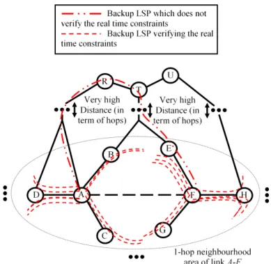
Fig. 9. Risk neighbourhood
Annex (relation between network size, locality and xλ value)
Contrarily to the value of the threshold which can be determined easily when the maximal quantity of bandwidth that a LSP can claim is known (otherwise, the ad-ministrator can associate a low value to the threshold), the optimal value of xλ
depends on several parameters like:
(1) the traffic matrix (traffic homogeneity),
(2) the protection link capacities (or link capacities when the bandwidth is not separated into two pools),
(3) the computation algorithm,
(4) the maximum ratio of protection requests that can be rejected,
(5) the topology network, the number of risks NR (especially node and SRLG risks) to be protected (0 < xλ≤ NR) and the structures of the SRLGs,
(6) etc.
In this section, we will concentrate on the impact of the increase of the network size (or on the impact of the increase of the number of network risks) on the value of xλ. To show that our approach scales when the network size increases (or when
the number of network risks increases), we try to determine an upper bound (UBλ)
for the value of xλ beyond which there is no bandwidth waste (or the bandwidth
waste is lower than a given constant). We note that this upper bound must not depend linearly on the network size (or on NR). In general, it does not correspond to the optimal value of xλ ; it ensures only that independently of the network size
(or independently on NR), the advertisement of a xλ vector of size equal to UBλ
avoids the reject by mistake of the arc λ when a new backup LSP is computed. Although there are some rare cases in theory where the value of UBλ depends
linearly on the network size (or on NR), the locality of protection ensures that the upper bound (UBλ) does not depend in practice on the network size but only on
the number of risks in the neighbourhood (for instance : 1-hop neighbourhood or 2-hop neighbourhood) of the arc λ.
Consider the example shown in figure 9 where all the arcs have the similar pro-tection capacity5. To protect against the failure of a given risk r, all the arcs and
nodes of the network topology, except those belonging to r, can be used. Typically, to compute a new backup LSP b protecting against the failure of the link A-F in figure 9, we can elect any link l (such as l 6= A-F) to be in the backup LSP b.
In order to decrease the amount of resources (MPLS labels, RSVP-TE states, etc.) reserved for the backup LSPs and to ensure acceptable recovery times (to satisfy the application time constraints)6, the backup LSP nodes should be close to the PLR
(PLR is always an end node of the protected link) and to the (next) next hop of the PLR (facility backup protection) or to the primary destination node (one-to-one backup protection). For instance, in figure 9, any backup LSP formed exclusively of arcs located in the 1-hop neighbourhood area of the protected link A-F is preferred to the LSP A-B-..-R-T-..-E-F because the very long length of the last LSP can result in the violation of the real time constraints of the supported communications. As a result, the links whose end nodes are far from the protected link/node are not (or are rarely) selected to be in a backup LSP protecting against the failure of that link/node although they verify the bandwidth constraints. We note that the exploration of a larger neighbourhood area to establish a new backup LSP does not generally decrease the blocking probability since this last metric depends strongly on the adjacent links of the head-end router of the backup LSP that is being computed (generally, the overloaded links which result in the rejection of a new backup LSP are those located in the 1-hop or 2-hop neighbourhood area of the PLR). Therefore, the number of risks whose protection cost is high on a given arc λ is in practice limited and depends generally on the close neighbourhood area (close nodes) of the arc λ (see figure 9 where almost all the backup LSPs verifying the real time constraints and protecting against the failure of link A-F are located in the 1-hop neighbourhood area of this link).
5 For simplicity, we considered that all the links have the same protection capacity. Same
conclusions can be obtained even when the protection capacities of the arcs are different.