HAL Id: hal-01632904
https://hal.archives-ouvertes.fr/hal-01632904
Submitted on 10 Nov 2017
HAL is a multi-disciplinary open access
archive for the deposit and dissemination of sci-entific research documents, whether they are pub-lished or not. The documents may come from teaching and research institutions in France or abroad, or from public or private research centers.
L’archive ouverte pluridisciplinaire HAL, est destinée au dépôt et à la diffusion de documents scientifiques de niveau recherche, publiés ou non, émanant des établissements d’enseignement et de recherche français ou étrangers, des laboratoires publics ou privés.
Dynamic Time Warping
Saeid Soheily-Khah, Pierre-François Marteau
To cite this version:
Saeid Soheily-Khah, Pierre-François Marteau. Sparsification of the Alignment Path Search Space in Dynamic Time Warping. Applied Soft Computing, Elsevier, In press, 78, pp.630 - 640. �10.1016/j.asoc.2019.03.009�. �hal-01632904�
Sparsification of the Alignment Path Search Space
in Dynamic Time Warping
Saeid Soheily-Khah, Pierre-Franc¸ois Marteau, Member, IEEE,
IRISA, CNRS, Universit´e Bretagne-Sud, Campus de Tohannic, Vannes, France
Abstract
Temporal data are naturally everywhere, especially in the digital era that sees the advent of big data and internet of things. One major challenge that arises during temporal data analysis and mining is the comparison of time series or sequences, which requires to determine a proper distance or (dis)similarity measure. In this context, the Dynamic Time Warping (DTW) has enjoyed success in many domains, due to its ’temporal elasticity’, a property particularly useful when matching temporal data. Unfortunately this dissimilarity measure suffers from a quadratic computational cost, which prohibits its use for large scale applications. This work addresses the sparsification of the alignment path search space for DTW-like measures, essentially to lower their computational cost without loosing on the quality of the measure.
As a result of our sparsification approach, two new (dis)similarity measures, namely SP-DTW (Sparsified-Paths search space DTW) and its kernelization SP-Krdtw (Sparsified-Paths search space Krdtw kernel) are proposed for time series comparison. A wide range of public datasets is used to evaluate the efficiency (estimated in term of speed-up ratio and classification accuracy) of the proposed (dis)similarity measures on the 1-Nearest Neighbor (1-NN) and the Support Vector Machine (SVM) classification algorithms. Our experiment shows that our proposed measures provide a significant speed-up without loosing on accuracy. Furthermore, at the cost of a slight reduction of the speedup they significantly outperform on the accuracy criteria the old but well known Sakoe-Chiba approach that reduces the DTW path search space using a symmetric corridor.
Index Terms
Temporal data, Dynamic Time Warping, 1-NN classification, SVM classification, Algorithmic complexity, Search space sparsification.
I. INTRODUCTION
D
UE to rapid increase in data size, the need for efficient temporal data mining has become morecrucial and time consuming during the past decade. Temporal data naturally appears in many emerging applications such as sensor networks, network security, medical data, e-marketing, dynamic social networks, human mobility, internet of things, etc. They can be time series or sequences of time stamped events or even purely sequential data such as strings or DNA sequences. In general, temporal data refers to data characterized by changes over time and the presence, unlike static data, of temporal dependency among them. Therefore the appropriate processing for data dependency or correlation analysis becomes vital in all temporal data processing.
This is in part why temporal data mining has recently attracted considerable attention in the data mining community [1]–[4]. Typically temporal data mining is concerned with the analysis of temporal data for finding temporal patterns and regularities in sets of temporal data, to define appropriate (dis)similarity measures with temporal alignment capabilities, to extract ”hidden” (temporal) structures, classify temporal objects, predict a future horizon and so on. Since it brings together techniques from different fields such as statistics, machine learning and databases, the literature is diffused among many different sources.
One main problem that arises during the temporal analysis is the choice or the design of a proper and accurate distance or (dis)similarity measure between time series (or sequences). There has been a very active research on how to properly define the concept of ”distance”, the ”similarity” or the ”dissimilarity” between time series and sequences. Sometimes two time series (or sequences) sharing the same configuration are considered close and their appearances are similar in terms of form, even
if they have very different values. However the value-based proximity measures are the most studied approaches to compare the time series (or sequences). Thus, a crucial issue is establishing what we mean by ”similar” or ”dissimilar” series due to their dynamic characters (with or without considering delay or temporal distorsion).
Different approaches to define the distance and the (dis)similarity between time series (or sequences) have been proposed in the literature [5]–[12], and for a recent review [13]. Among these works, Dynamic Time Warping (DTW) [14]–[16] has been largely popularized, studied and used in numerous applications. However, one of the main disadvantage of this measure is its quadratic computing cost that should be compared to the linear complexity of the Euclidean distance that can handle any feature sets containing also temporal or sequential features such as shapelets for instance.
The main contribution of this work is to propose a new approach to speed-up the computation of DTW, based on the sparsification of the admissible alignment path search space. Our contribution results in the description of the sparsification method and the proposal for two new (dis)similarity measures, namely SP-DTW (Sparsified-Paths search space DTW) and its kernelization SP-Krdtw (Sparsified-Paths search space Krdtw kernel). A detailed experimentation is proposed to assess our contribution against the state of the art approaches, dedicated to speed-up elastic distance computation.
The remainder of the paper is organized as follows: in the next section, a short overview of well-established (dis)similarity measures are presented, including time elastic measures. Next, in Section 3, we introduce the definition of the proposed sparsification of the alignment path search space that characterized time elastic measures. Then we introduce two new (sparsified path search space) measures that exploit this sparsification technique. Later, in Section 3, the conducted comparative experiments and results are discussed. Lastly, Section 4 concludes the paper.
II. TIMES SERIES BASIC MEASURES
Mining and comparing time series address a large range of challenges, among them: the meaningfulness of the distance and (dis)similarity measure. This section is dedicated to briefly describe the major well-known measures in a nutshell, which have been grouped into two categories: behavior-based and value-based measures [17].
A. Behavior-based measures
In this category, time series are compared according to their behaviors (or shapes). That is the case when time series of a same class exhibit similar behavior (or shapes), and time series of different classes have different behaviors (or shapes). In this context, we should define which time series are more similar to each other and which ones are different. The Main techniques to recover time series behaviors are: slopes and derivatives comparison, ranks comparison, Pearson and temporal correlation coefficients, and difference between auto-correlation operators. Here, we briefly describe some well-used behavior-based measures.
1) Pearson CORRelation coefficient (CORR): Let X = {x1, ..., xN} be a set of time series xi =
(xi1, ..., xiT) , i ∈ {1, ..., N }. The correlation coefficient between the time series xi and xj is defined by:
CORR(xi, xj) = T X t=1 (xit − xi)(xjt − xj) v u u t T X t=1 (xit− xi) 2 v u u t T X t=1 (xjt− xj) 2 (1) and
xi = T1 T X
t=1 xit
Correlation coefficient was first introduced by Bravais and later, Pearson in [18] illustrated that it is the best possible correlation between two time series. Up until now, many applications in different domains such as speech recognition, system design control, functional MRI and gene expression analysis have used the Pearson correlation coefficient as a behavior proximity measure between the time series (and sequences) [19]–[23]. The Pearson correlation coefficient changes between −1 and +1. The case CORR= +1, called perfect positive correlation, occurs when two time series perfectly coincide, and the case CORR= −1, called the perfect negative correlation, occurs when they behave completely opposite. CORR= 0 shows that the time series have different behavior. Observe that the higher correlation coefficient does not conclude the similar dynamics.
2) Difference Auto-Correlation Operators (DACO): The Auto-correlation is a representation of the
degree of similarity which measures the dependency between a time series and a shifted version of itself over successive time intervals. The Difference Auto-Correlation Operators (DACO) between the two time series xi and xj defined by [24]:
DACO(xi, xj) = k˜xi− ˜xjk2 (2) where, ˜ xi= (ρ1(xi), ..., ρk(xi)) , ρτ(xi) = T−τ X t=1 (xit− xi)(xi(t+τ ) − xi) T X t=1 (xit − xi) 2
and τ is the time lag. So, DACO compares time series by computing the distance between their dynamics, modeled by the auto-correlation operators. It is worth mentioning that the lower DACO does not represent the similar behavior.
B. Value-based measures
In this category, time series are compared according to their time stamped values. This subsection relies on two standard well-known sub-division: (a) without temporal warping (e.g. Minkowski distance) and (b) with considering temporal warping (e.g. Dynamic Time Warping).
1) Without temporal warping: The most used distance function in many applications is the Euclidean
(or Euclidian), which is commonly accepted as the simplest distance between sequences. The Euclidean distance dE (L2 norm) between two time series xi = (xi1, ..., xiT) and xj = (xj1, ..., xjT) of length T , is defined by: dE(xi, xj) = v u u t T X t=1 (xit− xjt) 2 (3)
The generalization of Euclidean Distance is Minkowski Distance, called Lp norm, and is defined by:
dLp(xi, xj) = p v u u t T X t=1 (xit− xjt) p
where p is called the Minkowski order. In fact, for Manhattan distance p = 1, for the Euclidean distance
p = 2, while for the Maximum distance p = ∞. All the Lp-norm distances do not consider the delay and
time warp. Unfortunately, they do not correspond to a common understanding of what a time series (or a sequence) is, and can not capture the flexible similarities.
2) With considering temporal warping: Searching the best alignment which matches two time series
is a crucial task for many applications. One of the eminent techniques to solve this task is Dynamic Time Warping (DTW); it was introduced in [14]–[16], with the application in speech recognition. DTW finds the optimal alignment between two time series, and captures the similarities by aligning the elements inside both series. Intuitively, the series are warped non-linearly in the time dimension to match each other. Simply, the DTW is a generalization of Euclidean distance which allows a non-linear mapping between two time series by minimizing a global alignment cost between them. DTW does not require that the two time series data have the same length, and also it can handle the local time shifting by duplicating (or re-sampling) the previous element of the time sequence.
Let X = {xi}Ni=1 be a set of time series xi = (xi1, ..., xiT) assumed of length T1. An alignment π of
length |π| = m between two time series xi and xj is defined as the set of m (T ≤ m ≤ 2T − 1) couples
of aligned elements of xi to elements of xj:
π = ((π1(1), π2(1)), (π1(2), π2(2)), ..., (π1(m), π2(m)))
where π defines a warping function that realizes a mapping from time axis of xi onto time axis of xj,
and the applications π1 and π2 defined from {1, ..., m} to {1, .., T } obey to the following boundary and
monotonicity conditions: 1 = π1(1) ≤ π1(2) ≤ ... ≤ π1(m) = T 1 = π2(1) ≤ π2(2) ≤ ... ≤ π2(m) = T and ∀ l ∈ {1, ..., m}, π1(l + 1) ≤ π1(l) + 1 and π2(l + 1) ≤ π2(l) + 1, (π1(l + 1) − π1(l)) + (π2(l + 1) − π2(l)) ≥ 1
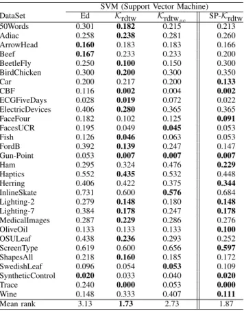
Intuitively, an alignment π defines a way to associate all elements of two time series. The alignments can be described by paths in the T × T grid as displayed in Figure 1, that crosses the elements of time series xi and xj. For instance, the green path aligns the two time series as: ((xi1, xj1), (xi2,xj2), (xi2,xj3), (xi3,xj4), ... , (xi6,xj6), (xi7,xj7)). In the following, we will denote A as the set of all possible alignments between two time series.
Fig. 1: Three possible alignments path (green, blue, yellow) between xi and xj
DTW is currently a well-known dissimilarity measure on time series (and sequences), since it makes
them possible to capture temporal distortions. The DTW between time series xi and time series xj, with
the aim of minimization of the mapping cost, is defined by:
DTW(xi, xj) = min π∈A X (t0,t)∈π ϕ(xit0, xjt) (4) 1
where ϕ : R × R → R+ is a real-valued positive divergence function (generally Euclidean norm).
While DTW alignments deal with delays or time shifting, the Euclidean alignment π between time
series xi and xj aligns elements observed at the same time:
π = ((π1(1), π2(1)), (π1(2), π2(2)), ..., (π1(T ), π2(T )))
where ∀t = 1, ..., T, π1(t) = π2(t) = t, |π| = T . According to the alignment definition, the euclidean
distance (dE) between the time series xi and xj is given by: dE(xi, xj) def === |π| X k=1 ϕ(xiπ1(k), xjπ2(k)) = T X t=1 ϕ(xit, xjt) where ϕ taken as the Euclidean norm.
Finally, Figure 2 shows the optimal alignment path between two sample time series with and without considering temporal warping. It has not escaped our notice that boundary, monotonicity and continuity are three important properties which are applied to the construction of the path. The boundary condition implies that the first elements of the two time series are aligned to each other, as well as the last elements. More precisely, the alignment is global and involves the entire time series. The monotonicity condition preserves the time-ordering of elements. In other word, the alignment path does not go back in ”time” index. Lastly, the continuity limits the warping path from long jumps and it guarantees that alignment does not omit important features.
Fig. 2: The optimal alignment path between two sample time series
with considering time warp or delay (left), without considering time warp or delay (right)
To find the minimum distance for alignment path, a dynamic programming approach is used. Let xi = (xi1, ..., xit) and xj = (xj1, ..., xjt0) two time series. A two-dimensional |xi| by |xj| cost matrix D is
built up, where the value at D(t, t0) is the minimun distance warp path that can be constructed from the
two time series xi and xj. Finally, the value at D(|xi|, |xj|) will contain the minimum distance between
the two time series under time warp. Be aware that the DTW is not a metric, since it does not satisfy the triangle inequality2.
2
As we can see, for instance, given three time series data, xi= [0], xj= [1, 2] and xk= [2,3,3], then:DTW(xi, xj) = 3 ,DTW(xj, xk) = 3
Time and space complexity of DTW are straightforward to derive. Each cell in the cost matrix is filled once in a constant time. The cost of the optimal alignment can be recursively computed by:
D(t, t0) = d(t, t0) + min{D(t − 1, t0), D(t − 1, t0− 1), D(t, t0− 1)}
where d is a distance function between the elements of time series, and these yield complexity of O(N2)
for the DTW. Hence, the standard DTW is much too slow for searching the optimal alignment path for large datasets. A lot of work has been proposed during the last 50 years to speed-up the DTW measure or variant of it. In general, the techniques which make DTW faster are divided in three main different categories:
1) constraints (e.g. Sakoe-Chiba band [25], [26]), 2) indexing (e.g. piecewise [27]),
3) data abstraction (e.g multiscale [28]).
Finally, in spite of the great success of DTW and its variants in a diversity of domains, there are still several persistent improvement needs about it, such as finding techniques to speed up DTW with no (or relaxed) constraints and make it more accurate.
3) Kernelization of DTW: Over the last ten years, estimation and learning methods using kernels have
become rather popular to cope with non-linearities, particularly in machine learning and data mining. More recently, several DTW-based kernels which allow one to process time series with kernel machines have been introduced [29]–[32], and they have been proved useful to handle and analyze structured data such as images, graphs, signals and texts [33]. However, such similarities (e.g. Kgdtw, Kdtak) cannot be translated easily into positive definite kernels, which is a vital requirement of kernel machines in the training phase [31], [32], [34]. Therefore, defining appropriate kernels to handle properly structured objects, and notably time series, remains a key challenge for researchers.
[31] introduced the global alignment kernel (Kga), that takes the following form: Kga(xi, xj) = X π∈P Y (t,t0)∈π κ(xit, xjt0) (5)
where κ(., .) is a local kernel and A the set of all admissible alignment paths.
In [32] another formal approach has been proposed to derive a positive definite time elastic kernel, Krdtw, close to the DTW matching scheme based on the design of a global alignment positive definite kernel for each single alignment path as given in Eq.6.
Krdtw(xi, xj) = X
π∈P⊂A
Kπ(xi, xj) (6)
where this time P is any subset of the set of all admissible alignment paths A between two time series, and Kπ(xi, xj) a positive definite kernel associated to path π and defined as:
Kπ(xi, xj) = Y (t,t0)∈π κ(xit, xjt0) + Y (t,t0)∈π κ(xit0, xjt) + Y (t,t0)∈π κ(xit, xjt) + Y (t,t0)∈π κ(xit0, xjt0) (7)
with κ a local kernel on Rd (typically κ(a, b) = e−ν·||a−b||2
).
Both kernels take into account not only (one of) the best possible alignment, but also all the good (or nearly the best) paths by summing up their global costs. The parameter ν is used to tune the local matches, thus penalizing more or less alignments moving away from the optimal ones. This parameter can be optimized by a grid/line search through a cross-validation.
The main advantage of Krdtw is that the restriction of the main summation over any subset P of A is guaranteed to be positive definite, which is not the case for Kga (even when P contains symmetric paths and the main diagonal path). As the sparsification of the DTW path search space involves to restrict the summation on subset of A, this property is quite relevant in an SVM classification context.
For both kernels, a dynamic programming computationally efficient solution exists, whose algorithmic
complexity is the same as the DTW (O(T2)), although the summation of products of exp functions is
more expensive than the evaluation of a min operation.
In summary, finding a suitable proximity measure is an important aspect when dealing with the time series (or sequences), that captures the essence of the them according to the domain of application. For instance, the Euclidean distance is commonly used due to its computational efficiency. However, it is very brittle for time series and small shifts of one time series can result in huge distance changes. Hence, more sophisticated distances and (dis)similarities have been devised to be more robust to small fluctuations of the input time series. Notably, the DTW and its kernalized variant have enjoyed success in many areas where its time complexity is not a critical issue.
III. SPARSIFIED-PATHS SEARCH SPACEDTW (SP-DTW)
The main idea behind this work is to introduce a kind of sparsification of the set of DTW alignment paths to make it faster to evaluate without degrading its accuracy by using an occupancy grid with the weighting values. The proposition mainly introduces a weighted warping function that constrains the search of the best alignment path in a subset of admissible alignments that has been learned and pruned on the trained data.
Let X = {xi}Ni=1 be a set of time series xi = (xi1, ..., xiT) assumed of length T , and πij be the optimal
alignment between two time series xi and xj expressed as the set of couples of aligned elements in the
T × T grid. Let mijtt0 be an indicative variable taking value 1 if path πij travels through the grid cell
with index tt0 (1 ≤ t, t0 ≤ T ), 0 otherwise. Then p(mtt0), which represents the normalized frequency of
occupancy of tt0 cell is defined by:
p(mtt0) = X i,j∈N mijtt0 X t,t0∈T X i,j∈N mijtt0 (8)
Hence, each cell in the occupancy grid has a value representing the frequency of the occupancy of that cell over all the optimal alignment paths in the training set. The higher values represent a high likeliness that an optimal alignment path, randomly drawn from the train set, contains that cell, and the values close to 0 represent a high likeliness that this optimal alignment path will not cross the cell. The proposed extended form of DTW, called Sparsified-Paths search space Dynamic Time Warping (SP-DTW), is then defined as:
SP-DTW(xi, xj) = min π∈P⊂A X (t,t0)∈π f (p(mtt0)) ϕ(xi t, xjt0) | {z } C(π) (9) = C(π∗)
where P is any subset of the set of all admissible alignment paths A between two time series, and
ϕ : R × R → R+ is a positive, real-valued, dissimilarity function (e.g. Euclidean distance).
For function f (p(mtt0)), we consider here p(mtt0)−γ, where γ ∈ R+∪ {0} controls the influence of the
weighting scheme. The negative exponent guarantees that the most important cells are privileged in the optimal alignment that minimizes the SP-DTW. For γ = 0, Eq. 9 leads to the standard DTW.
The cost function C computes the sum of the weighted dissimilarities ϕ between time series xi and
xj through the alignment π. The fact that f is non-increasing guarantees that the most important cells
(i.e. the cells with the higher frequencies) of the grid should be privileged in the optimal alignment
that minimizes the cost function C. Lastly, the optimal alignment path π∗ is obtained through the same
dynamic programming procedure as the one used for the standard DTW.
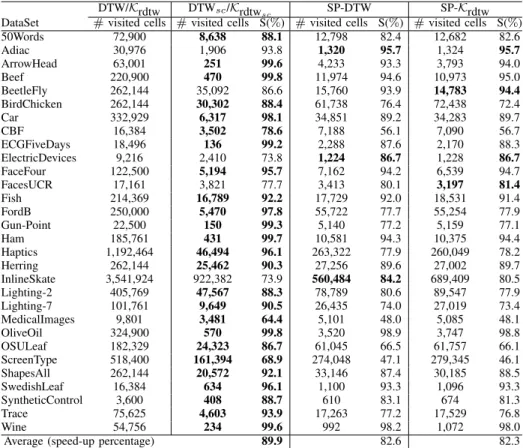
Fig. 3: The strategy of estimating sparse alignment global matrix: (a) the time series dataset, (b) the best pairwise alignment paths matrices, (c) the global alignment path matrix (resulting from the summation of all previous matrices), (d) cells that are not visited by an optimal path are set to 0 and the matrix is scaled into [0;1), (e) the cells with an occupancy frequency below θ are set to 0, (f) the sparse representation of the resulting global alignment matrix.
Figure 3 shows the strategy steps used to estimate the occupancy frequencies. Given a set of time series (Figure 3-a), we compute the pairwise alignment path between all the times series in the set. The grid cells, which are occupied by the path in each pairwise alignment, get the value 1, and the rest get the
value 0 (Figure 3-b). To be more efficient, instead of computing N2 pairwise comparison of DTW on
a dataset of N time series, we compute N (N − 1)/2 pairs of DTW, then we symmetrize the matrices
and get the same result as computing the N2 DTW pairwise comparison. In the next step, we sum all
the pairwise Boolean grids to obtain the global absolute frequency symmetric matrix that corresponds to the all of pairwise alignments (Figure 3-c). Then, to get the normalized frequency matrix, we normalize the global matrix in the range of [0 , 1)(Figure 3-d). To decrease the time and space complexity, we
Algorithm 1 SP-DTW
1: function SP-DTW(X, Y, [W, rw, cw])
. X,Y: two time series
. [W, rw, cw] sparse path alignment matrix
. W : weight vector, rw: row index vector, cw: column index vector
2: L← length of W . W , cw and rw have the same length
3: Lx ← length of X
4: Ly ← length of Y
. Initialize D, a (Lx× Ly) matrix, with Max Float values
5: D ← M ax F loat · ones(Lx, Ly) 6: D(1, 1) ← ||X(1) − Y (1)||2 · W (1) 7: for i = 2 to L do 8: ii ← rw(i) 9: jj ← cw(i) 10: if jj = 1 then
11: D(ii, 1) ← D(ii − 1, 1) + ||X(ii) − Y (1)||2· W (i)
12: else if ii = 1 then
13: D(1, jj) ← D(1, jj − 1) + ||X(1) − Y (jj)||2· W (i)
14: else
15: D(ii, jj) ← ||X(ii) − Y (jj)||2· W (i)+
16: Min(D(ii − 1, jj − 1), D(ii − 1, jj), D(ii, jj − 1))
17: Return D(Lx, Ly)
consider a threshold value θ for the frequency value of grid cells. The values smaller than the pre-defined threshold will be equal to zero (Figure 3-e). In practice, θ is estimated on the train data using a leave one out procedure. Lastly, we filter out the grid cells with zero weight to obtain a sparsified global matrix (Figure 3-f).
In practice, the sparsified alignment path matrix is stored as a list of coordinate (column, row, value) tuples. We denote this list as LOC. The entries of this list are sorted by increasing row index, then increasing column index, such that the sparsified variant of DTW (SP-DTW) can be iteratively evaluated according to Algorithm 1.
IV. SPARSIFIED-PATHS SEARCH SPACEDTW KERNEL(SP-KRDTW)
As already mentioned, we straightforwardly derive a positive definite time elastic kernel for sparsified subsets of alignment paths from Krdtw itself (Eq. 6), where P ⊂ A in Eq. 6 determines the sparsity of the path search space.
Note that, as Kπ(x, y) is proved to be a positive definite (p.d.) kernel [32], for all subset P ⊂ A,
SP-Krdtw, expressed as the sum of p.d. kernels3, is guaranteed to be p.d., which is not the case for a
sparsification of the global alignment kernel proposed in [31], even if P contains symmetric paths (if π ∈ P then π ∈ P, where π is the symmetric path of π) and the main diagonal ((1, 1), (2, 2) · · · (T, T ) ∈ P).
Here again, the sparsified subset of alignment paths P is characterized by the alignment path matrix that is stored as a list of coordinates (column, row, value) tuples (cf. Fig.3 (f)). Contrary to the SP-DTW algorithm, for the kernelized version, the weight values are not used, essentially to maintain the definiteness of the sparse kernel. As for SP-DTW the entries of this list are sorted by increasing row
3 Kπ(x, y) = Y (t,t0 )∈π κ(xt, yt0) + Y (t,t0 )∈π κ(xt0, yt) | {z } K1 + Y (t,t0 )∈π κ(xt, yt) + Y (t,t0 )∈π κ(xt0, yt0) | {z } K2 (cf. Eq.7)
Algorithm 2 SP-Krdtw
1: function SP-Krdtw(X, Y, ν, rw, cw) . X, Y : two time series
. ν: Krdtw parameter
. We note κν(x, y) = exp(−ν · ||x − y||2), the local kernel
. [rw, cw] sparse path alignment matrix indices (row and column index vectors)
2: L ← length of rw . cw and rw have the same length
3: Lx ← length of X
4: Ly ← length of Y
. Initialize K1 and K2, two (Lx× Ly) matrices, with zero values
5: K1 ← zeros(Lx, Ly) 6: K2 ← zeros(Lx, Ly) 7: K1(1, 1) ← κν(X(1), Y (1)) 8: K2(1, 1) ← κν(X(1), Y (1)) 9: for i = 1 to L do 10: if (i < Lx and i < Ly) then 11: for i = 2 to L do 12: ii ← rw(i) 13: jj ← cw(i) 14: if jj = 1 then
15: K1(ii, 1) ← 1.0/3.0 · K1(ii − 1, 1) · κν(X(ii), Y (1))
16: K2(ii, 1) ← 1.0/3.0 · K2(ii − 1, 1) · κν(X(ii), Y (ii))
17: else if ii = 1 then
18: K1(1, jj) ← 1.0/3.0 · K1(1, jj − 1) · κν(X(1), Y (jj))
19: K2(1, jj) ← 1.0/3.0 · K2(1, jj − 1) · κν(X(jj), Y (jj))
20: else
21: K1(ii, jj) ← 1.0/3.0 · κν(X(ii), Y (jj))·
22: (K1(ii − 1, jj − 1) + K1(ii − 1, jj) + K1(ii, jj − 1))
23: K2(ii, jj) ← 1.0/3.0 · (κν(X(ii), Y (ii)) + κν(X(jj), Y (jj)))/2 · K2(ii − 1, jj − 1)+
24: K2(ii − 1, jj) · κν(X(ii), Y (ii)) + K2(ii, jj − 1) · κν(X(jj), Y (jj))
25: Return K1(Lx, Ly) + K2(Lx, Ly)
index, then increasing column index, such that the sparsified Krdtw kernel can be evaluated iteratively as presented in Algorithm 2.
While the complexity of computing the DTW is quadratic in T (the length of the time series), for Sparse-Paths versions, the complexity is linear with the number of non-zero cells of the path matrix. Hence the
algorithmic complexity for SP-DTW and SP-Krdtw are in between O(T ) and O(T2). Furthermore, the
sparse data is by nature more easily compressed and thus may require significantly less storage. V. EXPERIMENTAL STUDY
In this section, we first describe the datasets retained to lead our experiments prior to comparing the Nearest Neighbor (1-NN) and Support Vector Machine (SVM) classification algorithms, based on the proposed (dis)similarity measures comparatively with some of the most known and well-used alternative ones.
A. Data sets description
Our experiments are conducted on 30 public datasets from UCR time series classification archive [47]. Table I describes the datasets considered, with their main characteristics: number of categories (k),
dataset train and test size (N) and time series length (T), where classes composing the datasets are known beforehand. The datasets retained have very diverse structures and shapes, and as can be seen, they come in different class numbers, train and test set sizes as well as time series lengths.
TABLE I: Data description
Class Nb. Size (Train) Size (Test) TS. Length
DataSet k N N T 50Words 50 450 455 270 Adiac 37 390 391 176 ArrowHead 3 36 175 251 Beef 5 30 30 470 BeetleFly 2 20 20 512 BirdChicken 2 20 20 512 Car 4 60 60 577 CBF 3 30 900 128 ECGFiveDays 2 23 861 136 ElectricDevices 7 8926 7711 96 FaceFour 4 24 88 350 FacesUCR 14 200 2050 131 Fish 7 175 175 463 FordB 2 810 3636 500 Gun-Point 2 50 150 150 Ham 2 109 105 431 Haptics 5 155 308 1092 Herring 2 64 64 512 InlineSkate 7 100 550 1882 Lighting-2 2 60 61 637 Lighting-7 7 70 73 319 MedicalImages 10 381 760 99 OliveOil 4 30 30 570 OSULeaf 6 200 242 427 ScreenType 3 375 375 720 ShapesAll 60 600 600 512 SwedishLeaf 15 500 625 128 SyntheticControl 6 300 300 60 Trace 4 100 100 275 Wine 2 57 54 234 B. Validation protocol
Here we compare the 1-NN and SVM classification algorithms based on the proposed (dis)similarity measures (SP-DTW and SP-Krdtw) with the classical CORR, DACO, Ed, DTW measures as well as the
DTWsc and Krdtw. We focus on the above measures because they constitute the most frequently used
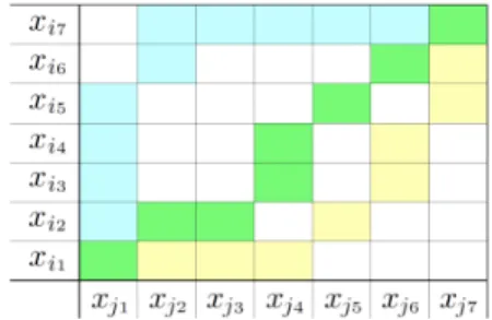
proximity measure and distance metrics in temporal data mining. For our comparison in this paper, we rely on the classification error rate, which measures the agreement between the predicted class labels and the actual ones, to evaluate each metric, and the time speed-up percentage. The classification error rate lies in [0, 1] and the lower index, the better the agreement is. In particular, the best value of error rate, 0, is reached when the predicted class labels are equivalent to the actual class labels. Finally, the meta parameters used in some of the measures (e.g. τ , the time lag in DACO, θ, the threshold value in SP-DTW, or ν in Krdtw) are selected according to a k-fold cross validation set or a leave one out procedure through a standard grid search process carried out on the train data. For instance, Figure 4 shows the threshold estimation for some sample dataset using the error rate of leave one out procedure through a grid/line search. The lower error rate value indicates the optimal threshold.
Fig. 4: The error rate diagram of the leave one out procedure through a grid/line search in the range of [0, 15] on the train dataset 50words (left), facesUCR (middle), and wine (right)
C. Experimental results
The error rate for 1-NN classification for each distance or (dis)similarity, on each dataset, are reported in Table II. Results in bold correspond to the best values.
TABLE II: Comparison of 1-NN classification error rate
1-NN (Nearest Neighbor)
BEHAVIOR-BASED VALUE-BASED
DataSet CORR DACO Ed DTW DTWsc Krdtw SP-DTW SP-Krdtw
50Words 0.369 0.261 0.369 0.310 0.242(6) 0.196 0.226 0.202 Adiac 0.389 0.445 0.389 0.396 0.391(3) 0.379 0.391 0.368 ArrowHead 0.200 0.234 0.200 0.297 0.200(0) 0.200 0.217 0.194 Beef 0.333 0.367 0.333 0.367 0.333(0) 0.367 0.267 0.333 BeetleFly 0.250 0.250 0.250 0.300 0.300(7) 0.300 0.250 0.300 BirdChicken 0.450 0.300 0.450 0.250 0.300(6) 0.250 0.250 0.150 Car 0.267 0.283 0.267 0.267 0.233(1) 0.183 0.183 0.183 CBF 0.148 0.232 0.148 0.003 0.004(11) 0.002 0.014 0.002 ECGFiveDays 0.203 0.202 0.203 0.232 0.203(0) 0.124 0.189 0.091 ElectricDevices 0.450 0.434 0.450 0.399 0.376(14) 0.384 0.394 0.376 FaceFour 0.216 0.193 0.216 0.170 0.114(2) 0.114 0.114 0.102 FacesUCR 0.231 0.192 0.231 0.095 0.088(12) 0.067 0.080 0.067 Fish 0.217 0.265 0.217 0.177 0.154(4) 0.086 0.177 0.086 FordB 0.442 0.261 0.442 0.406 0.414(1) 0.410 0.395 0.413 Gun-Point 0.087 0.067 0.087 0.093 0.087(0) 0.027 0.027 0.027 Ham 0.400 0.514 0.400 0.533 0.400(0) 0.400 0.400 0.371 Haptics 0.630 0.636 0.630 0.623 0.588(2) 0.471 0.584 0.542 Herring 0.484 0.500 0.484 0.469 0.469(5) 0.406 0.421 0.375 InlineSkate 0.658 0.680 0.658 0.616 0.613(14) 0.562 0.592 0.562 Lighting-2 0.246 0.197 0.246 0.131 0.131(6) 0.098 0.114 0.098 Lighting-7 0.425 0.382 0.425 0.274 0.288(5) 0.247 0.260 0.219 MedicalImages 0.316 0.330 0.316 0.263 0.253(20) 0.265 0.257 0.240 OliveOil 0.133 0.167 0.133 0.167 0.133(0) 0.133 0.133 0.167 OSULeaf 0.479 0.422 0.479 0.409 0.388(7) 0.306 0.384 0.302 ScreenType 0.640 0.669 0.640 0.603 0.589(17) 0.613 0.589 0.592 ShapesAll 0.248 0.280 0.248 0.232 0.198(4) 0.177 0.223 0.173 SwedishLeaf 0.211 0.162 0.211 0.208 0.154(2) 0.158 0.123 0.137 SyntheticControl 0.120 0.353 0.120 0.007 0.017(6) 0.003 0.010 0.007 Trace 0.240 0.140 0.240 0.000 0.010(3) 0.010 0.000 0.010 Wine 0.389 0.407 0.389 0.426 0.389(0) 0.370 0.351 0.351 Mean rank 5.37 6.27 5.37 5.03 3.53 2.30 2.63 1.73
Based on the classification error rate displayed in Table II, one can note that 1-NN classification with SP-Krdtw leads to the best classification results overall (20 datasets out of 30). This is highlighted in the last row of the table which presents the mean rank position for each tested method. In particular, one shown the DTW with Sakoe-Chiba corridor is outperformed by our two proposed measures. Furthermore, from Table II, one can experimentally verify that the 1-NN classification based on the Pearson correlation coefficient (CORR) has the same error rate with the 1-NN based on the Euclidean distance (Ed). This is theoretically verified in the Appendix A.
TABLE III: Wilcoxon signed-rank test of pairwise error rate differences for 1-NN Method DACO DTW DTWsc Krdtw SP-DTW SP-Krdtw CORR/Ed 0.9225 0.0125 p<0.0001 p<0.0001 p<0.0001 p<0.0001 DACO - 0.0296 0.0002 p<0.0001 p<0.0001 p<0.0001 DTW - - 0.0012 p<0.0001 p<0.0001 p<0.0001 DTWsc - - - 0.0012 0.0068 0.0001 Krdtw - - - - 0.0011 0.0189 SP-DTW - - - 0.0249
In Table III we report the P-values for each pair of tested algorithms using a Wilcoxon signed-rank test. The null hypothesis is that for a tested pair of classifiers, the difference between classification error rates obtained on the 30 datasets follows a symmetric distribution around zero. With a 0.01 significance level, the P-values that lead to reject the null hypothesis are shown in bolded fonts in the table. It turns out that SP-Krdtw performs significantly better than all the other tested measures except for Krdtw since the differences between them is not significant according to the Wilcoxon signed-rank test. Furthermore, the differences between SP-Krdtw and SP-DTW are not significant, but both measures are significantly better
than DTWsc and the remaining measures (except Krdtw). Hence, the learned sparsification of alignment
paths outperforms significantly the well-used Sakoe-Schiba DTW with adjusted corridor.
TABLE IV: Comparison of SVM classification error rate
SVM (Support Vector Machine)
DataSet Ed Krdtw Krdtw sc SP-Krdtw 50Words 0.301 0.182 0.215 0.213 Adiac 0.258 0.238 0.281 0.260 ArrowHead 0.160 0.183 0.183 0.166 Beef 0.167 0.233 0.233 0.200 BeetleFly 0.250 0.100 0.150 0.300 BirdChicken 0.300 0.200 0.300 0.350 Car 0.200 0.217 0.200 0.133 CBF 0.116 0.002 0.004 0.002 ECGFiveDays 0.028 0.019 0.072 0.022 ElectricDevices 0.406 0.280 0.365 0.365 FaceFour 0.182 0.102 0.125 0.091 FacesUCR 0.195 0.049 0.045 0.053 Fish 0.126 0.046 0.063 0.053 FordB 0.392 0.139 0.247 0.147 Gun-Point 0.053 0.007 0.007 0.007 Ham 0.295 0.324 0.476 0.229 Haptics 0.552 0.435 0.532 0.448 Herring 0.406 0.422 0.375 0.344 InlineSkate 0.731 0.600 0.576 0.684 Lighting-2 0.279 0.148 0.180 0.148 Lighting-7 0.384 0.178 0.247 0.178 MedicalImages 0.287 0.229 0.286 0.276 OliveOil 0.133 0.133 0.133 0.100 OSULeaf 0.438 0.236 0.293 0.252 ScreenType 0.619 0.600 0.656 0.597 ShapesAll 0.218 0.160 0.185 0.172 SwedishLeaf 0.096 0.054 0.053 0.109 SyntheticControl 0.020 0.033 0.040 0.020 Trace 0.240 0.000 0.053 0.000 Wine 0.148 0.333 0.407 0.111 Mean rank 3.13 1.73 2.73 1.87
In addition, Table IV displays the performance of SVM classification over each measure on each dataset for further experiments. Similar as before, results in bold correspond to the best values. As can be seen, based on the SVM classification error rate, SVM with Krdtw leads to the best classification results overall (17 datasets out of 30), followed by SVM classification with SP-Krdtw (13 datasets out of 30). Here again, this is highlighted in the last row of the table which presents the mean rank position
for each tested method. One can see that the Krdtwsc (that involves a fixed-size Sakoe-Chiba corridor)
is outperformed by our proposed measure SP-Krdtw. To verify for significant differences, as above, we used the Wilcoxon signed-rank tests.
TABLE V: Wilcoxon signed-rank test of pairwise error rate differences for SVM Method Krdtw Krdtw sc SP-Krdtw Ed p<0.0001 0.0279 0.0002 Krdtw - 0.0002 0.5539 Krdtwsc - - 0.0097
Table V gives the P-values for the Wilcoxon signed-rank tests. With the same null hypothesis as above (difference between the error rates follows a symmetric distribution around zero), and with a 0.01 significance level, the P-values that lead to reject the null hypothesis are presented in bolded fonts in the tables. These tests show that no significance difference exists between Krdtw and SP-Krdtw, while
Krdtw and SP-Krdtw are significantly better than Ed and Krdtwsc. Here again, the learned sparsification
of alignment paths significantly outperforms the Sakoe-Chiba variant of the kernelized DTW (Krdtwsc)
with adjusted corridor on the train data.
As far as one can see in Table II until V, the best classification results are obtained by SP-Krdtw, SP-DTW and Krdtw. The main benefit is an important speed-up without loss of accuracy. To justify our speed-up claim, Table VI shows the complexity, expressed in terms of number of cell visited in the alignment path matrix, of the proposed paths search space sparsified measures in comparison with the standard DTW and its kernelization.
To do so, we consider the number of visited cells in the alignment path matrix, in each pairwise comparison, for each measure. While for standard DTW (or its kernelization), we need to consider the
whole grid cells (T2) for each time series pairwise comparison, the results illustrate that we dramatically
decreased the number of visited cells for each pairwise comparison in SP-DTW and SP-Krdtw. To justify, for each measure, we obtain the speed-up percentage (S), which is the number of visited cells divided
by the total number of grid cells (T2). As can be seen, for the proposed measure, we decline the cells
visited numbers more than 82% in average, while the speed-up is almost 89% for DTWsc or Krdtwsc.
TABLE VI: Comparison of time speed-up (in %) comparatively to the standard DTW (or Krdtw)
DTW/Krdtw DTWsc/Krdtw
sc SP-DTW SP-Krdtw
DataSet # visited cells # visited cells S(%) # visited cells S(%) # visited cells S(%)
50Words 72,900 8,638 88.1 12,798 82.4 12,682 82.6 Adiac 30,976 1,906 93.8 1,320 95.7 1,324 95.7 ArrowHead 63,001 251 99.6 4,233 93.3 3,793 94.0 Beef 220,900 470 99.8 11,974 94.6 10,973 95.0 BeetleFly 262,144 35,092 86.6 15,760 93.9 14,783 94.4 BirdChicken 262,144 30,302 88.4 61,738 76.4 72,438 72.4 Car 332,929 6,317 98.1 34,851 89.2 34,283 89.7 CBF 16,384 3,502 78.6 7,188 56.1 7,090 56.7 ECGFiveDays 18,496 136 99.2 2,288 87.6 2,170 88.3 ElectricDevices 9,216 2,410 73.8 1,224 86.7 1,228 86.7 FaceFour 122,500 5,194 95.7 7,162 94.2 6,539 94.7 FacesUCR 17,161 3,821 77.7 3,413 80.1 3,197 81.4 Fish 214,369 16,789 92.2 17,729 92.0 18,531 91.4 FordB 250,000 5,470 97.8 55,722 77.7 55,254 77.9 Gun-Point 22,500 150 99.3 5,140 77.2 5,159 77.1 Ham 185,761 431 99.7 10,581 94.3 10,375 94.4 Haptics 1,192,464 46,494 96.1 263,322 77.9 260,049 78.2 Herring 262,144 25,462 90.3 27,256 89.6 27,002 89.7 InlineSkate 3,541,924 922,382 73.9 560,484 84.2 689,409 80.5 Lighting-2 405,769 47,567 88.3 78,789 80.6 89,547 77.9 Lighting-7 101,761 9,649 90.5 26,435 74.0 27,019 73.4 MedicalImages 9,801 3,481 64.4 5,101 48.0 5,085 48.1 OliveOil 324,900 570 99.8 3,520 98.9 3,747 98.8 OSULeaf 182,329 24,323 86.7 61,045 66.5 61,757 66.1 ScreenType 518,400 161,394 68.9 274,048 47.1 279,345 46.1 ShapesAll 262,144 20,572 92.1 33,146 87.4 30,185 88.5 SwedishLeaf 16,384 634 96.1 1,100 93.3 1,096 93.3 SyntheticControl 3,600 408 88.7 610 83.1 674 81.3 Trace 75,625 4,603 93.9 17,263 77.2 17,529 76.8 Wine 54,756 234 99.6 992 98.2 1,072 98.0
Lastly, to have a closer look at the grid cells search space in time series pairwise comparison, in Figures 5 till 8, we plot the color-coded of occupancy grid cells of some sample datasets for the DTW (or Krdtw) with the optimal Sakoe-Chiba band and for the path sparsified measures with and without considering the threshold value, according to the frequency of occupancy over the optimal alignment paths in the training set.
Fig. 5: Beef: color-coded of grid cells DTW with optimal Sakoe-Chiba band (left), with sparse paths DTW (middle), with sparse paths DTW considering a threshold (right)
Fig. 6: BeetleFly: color-coded of grid cells DTW with optimal Sakoe-Chiba band (left), with sparse paths DTW (middle), with sparse paths DTW considering a threshold (right)
Fig. 7: ElectricDevices: color-coded of grid cells DTW with optimal Sakoe-Chiba band (left), with sparse paths DTW (middle), with sparse paths DTW considering a threshold (right)
Fig. 8: MedicalImages: color-coded of grid cells DTW with optimal Sakoe-Chiba band (left), with sparse paths DTW (middle), with sparse paths DTW considering a threshold (right)
VI. CONCLUSION
The Dynamic Time Warping (DTW) is among the most commonly used measure for temporal data comparison in several domains such as signal processing, image processing and pattern recognition. This research work proposes a sparsification of the alignment path search space for DTW-like measures and their kernelization Krdtw. This led us to propose two new (dis)similarity measures for temporal data analysis and comparison under time warp that cope with such kind of sparsity. For this, we propose an extension of the standard DTW and its kernelization, based on a weighting, learned over the optimal alignment paths in the training set and the sparsification of the admissible alignment path search space using a threshold on these weights. The efficiency of the proposed (dis)similarity measures, has been analyzed on a wide range of public datasets on two classification tasks: 1-NN and SVM (for the definite measures). The results show that the classification with path sparsified measures leads to an important speed-up without losing on the accuracy. In particular, these measures significantly outperform the DTW with a Sakoe-Chiba corridor whose size is optimized on the train data. Finally, we have shown that the kernelized version of DTW admits a straightforward path sparsification variant, much faster and with similar accuracy.
REFERENCES
[1] Bradley P. S. and Fayyad U. M.: Refining Initial Points for K-Means Clustering. ICML, Morgan Kaufmann Publishers Inc., Pages 91–99 (1998)
[2] Halkidi M., Batistakis Y. and Vazirgiannis M.: On Clustering Validation Techniques. Journal of Intelligent Information Systems, Pages 107–145 (2001)
[3] Kalpakis K., Gada D. and Puttagunta V.: Distance Measures for Effective Clustering of ARIMA Time-Series. ICDM, IEEE Computer Society, Pages 273–280 (2001)
[4] Keogh E., Lin J. and Truppel W.: Clustering of time series subsequences is meaningless. Implications for Previous and Future Research. ICDM, IEEE CS(2003)
[5] Moeckel R. and Murray B.: Measuring the distance between time series. Physica D: Nonlinear Phenomena, Vol 102, Number 3, Pages 187– 194 (1997)
[6] Gunopulos D.: Time series similarity measures. John Wiley & Sons, Ltd, Encyclopedia of Biostatistics, doi 10.1002/0470011815.b2a12074 (2004)
[7] Marteau P.-F.: Time Warp Edit Distance with Stiffness Adjustment for Time Series Matching. IEEE Transactions on Pattern Analysis and Machine Intelligence, Vol 31, Pages 306 – 318, doi 10.1109/TPAMI.2008.76 (2009)
[8] Batista G. and Wang X. and Keogh E. J.: A complexity-invariant distance measure for time series. SDM, SIAM / Omnipress, Pages 699–710, doi 10.1137/1.9781611972818.60 (2011)
[9] Cassisi C. and Pulvirenti A. and Cannata A. and Aliotta M. and Montalto P.: Similarity Measures and Dimensionality Reduction Techniques for Time Series Data Mining. INTECH Open Access Publisher (2012)
[10] Serr`a J. and Llu´ıs Arcos J.: An Empirical Evaluation of Similarity Measures for Time Series Classification. CoRR, Knowledge-Based Systems 67, Pages 305–314, doi 10.1016/j.knosys.2014.04.035 (2014)
[11] Li X., Makkie M., Lin B., Sedigh Fazli M., Davidson I., Ye J., Liu T. and Quinn Sh.: Scalable fast rank-1 dictionary learning for fmri big data analysis. Proceedings of the 22nd ACM SIGKDD International Conference on Knowledge Discovery and Data Mining, Pages 511–519 (2016)
[12] Soheily-Khah S., Douzal-Chouakria A. and Gaussier E.: Generalized k-means based clustering for temporal data under weighted and kernel time warp. Pattern Recognition Letter, Vol 75, Pages 63–69 (2016)
[13] Bagnall A., Lines J., Bostrom A., Large J. and Keogh E.: The great time series classification bake off: a review and experimental evaluation of recent algorithmic advances. Data Mining and Knowledge Discovery, Springer, Vol 31, Issue 3, Pages 606–660 (2017)
[14] Bellman R. and Dreyfus S.: Applied Dynamic Programming. Princeton Univ. Press (1962)
[15] Itakura F.: Minimum prediction residual principle applied to speech recognition. Acoustics, Speech and Signal Processing, IEEE, Vol 23, Pages 67–72 (1975)
[16] Kruskall J.B and Liberman M.: The symmetric time warping algorithm: From continuous to discrete. In Time Warps, String Edits and Macromolecules (1983)
[17] Soheily-Khah S.: Generalized k-means based clustering for temporal data under time warp. Universite Grenoble Alpes, https://hal.archives-ouvertes.fr/tel-01394280, Theses (2016)
[18] Pearson K.: Contributions to the mathematical theory of evolution. Trans. R. Soc. Lond. Ser., Pages 253–318 (1896)
[19] MacArthur B.D., Lachmann A., Lemischka I.R. and Ma’ayan A.: GATE: Software for the analysis and visualization of high-dimensional time series expression data. Bioinformatics, Vol 26, Pages 143–144 (2010)
[20] Ernst J., Nau G.J. and Bar-Joseph Z.: Clustering short time series gene expression data. Bioinformatics, Vol 21, Pages 159-168, (2005)
[21] Abraham Z. and Tan P.: An integrated framework for simultaneous classification and regression of time-series Data. SIAM ICDM, Pages 653–664 (2010)
[22] Cabestaing F., Vaughan T.M., McFarland D.J. and Wolpaw J.R.: Classification of evoked potentials by Pearson´ıs correlation in a Brain-Computer Interface. Modelling C Automatic Control (theory and applications), Vol 67, Pages 156–166 (2007)
[23] Rydell J., Borga M. and Knutsson H.: Robust Correlation Analysis with an Application to Functional MRI. IEEE International Conference on Acoustics, Speech and Signal Processing, Pages 453–456 (2008)
[24] Gaidon A., Harchaoui Z. and Schmid C.: A time series kernel for action recognition. British Machine Vision Conference (2011)
[25] Sakoe H. and Chiba S.: A dymanic programming approach to continuous speech recognition. Int. Congress on Acoustics, Vol 3, Pages 65 – 69 (1971)
[26] Sakoe H. and Chiba S.: Dynamic programming algorithm optimization for spoken word recognition. IEEE Transactions on Acoustics, Speech, and Signal Processing, Vol 26, Number 1, Pages 43 – 49 (1978)
[27] Keogh E.J. and Pazzani M.J.: Scaling Up Dynamic Time Warping for Data Mining Applications. ACM SIGKDD, Pages 285–289 (2000)
[28] Salvador S. and Chand Ph.: FastDTW: Toward Accurate Dynamic Time Warping in Linear Time and Space. KDD Workshop on Mining Temporal and Sequential Data, Pages 70–80 (2004)
[29] Bahlmann C., Haasdonk B., and Burkhardt H.: Online handwriting recognition with support vector machines-a kernel approach. Frontiers in Handwriting Recognition, Pages 49 – 54 (2002)
[30] Shimodaira H. and Noma K.I. and Nakai M. and Sagayama S.: Dynamic time-alignment kernel in support vector machine. NIPS, Vol 14, Pages 921 – 928 (2002)
[31] Cuturi M. and Vert J.-Ph. and Birkenes O. and Matsui T.: A kernel for time series based on global alignments. International Conference on Acoustics, Speech and Signal Processing, Vol 11, Pages 413 –416 (2007)
[32] Marteau P.-F. and Gibet S.: On Recursive Edit Distance Kernels With Application to Time Series Classification. IEEE Transactions on Neural Networks and Learning Systems, vol. 26, no. 6, pp. 1121-1133, June (2015)
[33] Hofmann T., Scholkopf B. and Smola A. J.: Kernel methods in machine learning. Annals of Statistics, Vol 36, Pages 1171–1220 (2008)
[34] Joder C. and Essid S. and Richard G.: Alignment kernels for audio classification with application to music instrument recognition. European Signal Processing Conference EUSIPCO, Pages 1–5 (2008)
[35] Das G. and Lin K. and Mannila H. and Renganathan G. and Smyth P.: Rule discovery from time series. Proceedings of th 4th International Conference of Knowledge Discovery and Data Mining, Pages 16–22, AAAI Press. (1998)
[36] Kadous M.W.: Learning comprehensible descriptions of multivariate time series. 16th International Machine Learning Conference, Pages 454–463, (1999)
[37] Diez J.J.R. and Gonzalez C.A.: Applying boosting to similarity literals for time series classification. Multiple Classifier Systems, Pages 210–219 (2000)
[38] Chu S. and Keogh E. and Hart D. and Pazzani M.: Iterative Deepening Dynamic Time Warping for Time Series. SIAM ICDM (2002)
[39] Ratanamahatana Ch. A. and Keogh E.: Making Time-series Classification More Accurate Using Learned Constraints. SDM, PAges 11–22 (2004)
[40] Mller M.:Dynamic Time Warping. Information Retrieval for Music and Motion, Chapter 4, Pages 69–84, doi 10.1007/978-3-540-74048-3 (2007)
[41] Rakthanmanon T.: Addressing big data time series: mining trillions of time series subsequences under dynamic time warping. ACM Transactions on Knowledge Discovery from Data. Vol 7, doi 10.1145/2510000/2500489 (2013)
[42] Izakian H. and Pedrycz W. and Jamal I.: Fuzzy clustering of time series data using dynamic time warping distance. Engineering Applications of Artificial Intelligence, Vol 39, Pages 235 – 244, doi 10.1016/j.engappai.2014.12.015 (2015)
[43] Yi B.K. and Jagadish H. and Faloutsos C.: Efficient retrieval of similar time sequences under time warping. ICDE, Pages 23–27 (1998)
[44] Caiani E.G. and Porta A. and Baselli G. and Turiel M. and Muzzupappa S. and Pieruzzi F. and Crema C. and Malliani A. and Cerutti S.: Warped-average template technique to track on a cycle-by-cycle basis the cardiac filling phases on left ventricular. IEEE Computers in Cardiology, Pages 73–76 (1998)
[45] Aach J. and Church G.: Aligning gene expression time series with time warping algorithms. Bioinformatics, Vol 17, Pages 495–508 (2001)
[46] Bar-Joseph Z. and Gerber G. and Gifford D. and Jaakkola T. and Simon I.: A new approach to analyzing gene expression time series data. International Conference on Research in Computational Molecular Biology, Pages 39–48 (2002)
[47] Chen Y. and Keogh E. and Hu B. and Begum N. and Bagnall A. and Mueen A. and Batista G.: The UCR Time Series Classification Archive. www.cs.ucr.edu/∼eamonn/time series data/ (2015)
APPENDIXA
The Pearson correlation coefficient between time series x and y are defined as follows: CORR(x,y) = COV(x,y)
σ(x)σ(y) (10)
Since, the numerator of the equation (COV), covariance of two time series, is the difference between the mean of the product of x and y subtracted from the product of the means, the Eq. 10 leads to:
CORR(x,y) = 1 T T X t=1 xtyt− µxµy σ(x)σ(y)
where µx and µy are the means of x and y respectively, and σ(x) and σ(y) are the standard deviations of
x and y.
Note that if x and y are standardized4, they will each have a mean of 0 and a standard deviation of 1,
so:
µx = µy = 0 σ(x) = σ(y) = 1 and the formula reduces to:
CORR(x,y) = 1 T T X t=1 xtyt (11)
Whereas the Euclidean distance is the sum of squared differences, the Pearson correlation is basically the average product. If we expand the Euclidean distance (Ed) formula, we get:
dE(x,y) = v u u t T X t=1 (xt− yt)2 = v u u t T X t=1 xt2+ T X t=1 yt2− 2 T X t=1 xtyt
But if x and y are standardized, the sumsPT
t=1xt2 and
PT
t=1yt2 are both equal to T. That leaves
PT
t=1xtyt as the only non-constant term, just as it was in the reduced formula for the Pearson correlation coefficient (Eq. 11).
Thus, for the standardized dataset, One can write the Pearson correlation between two time series in terms of the squared distance between them as:
CORR(x,y) = 1 − d2 E(x,y) 2T . .2 4

![Fig. 4: The error rate diagram of the leave one out procedure through a grid/line search in the range of [0, 15] on the train dataset 50words (left), facesUCR (middle), and wine (right)](https://thumb-eu.123doks.com/thumbv2/123doknet/12255039.320360/13.918.80.839.82.290/error-diagram-leave-procedure-search-dataset-facesucr-middle.webp)