Science Arts & Métiers (SAM)
is an open access repository that collects the work of Arts et Métiers Institute of
Technology researchers and makes it freely available over the web where possible.
This is an author-deposited version published in: https://sam.ensam.eu Handle ID: .http://hdl.handle.net/10985/8358
To cite this version :
David LESAGE, Jean-Claude LEON, Philippe VERON - Discrete curvature approximations and segmentation of polyhedral surfaces - International Journal of Shape Modeling - Vol. 11, n°2, p.217-252 - 2005
Any correspondence concerning this service should be sent to the repository Administrator : [email protected]
Discrete curvature approximations
and segmentation of polyhedral surfaces
D. Lesage, J-C. Léon, P. Véron*
Soils, Solids, Structure Laboratory, Integrated Design Project, UMR CNRS 5521
Domaine Universitaire, BP 53, 38041 GRENOBLE Cedex 9, France Email: [email protected], [email protected]
* Centre d’Etudes et de Recherches de l’Ecole Nationale Supérieure des Arts et Métiers
2 cours des Arts et Métiers, 13617 AIX EN PROVENCE, France Email: [email protected]
Abstract
The segmentation of digitized data to divide a free form surface into patches is one of the key steps required to perform a reverse engineering process of an object. To this end, discrete curvature approximations are introduced as the basis of a segmentation process that lead to a decomposition of digitized data into areas that will help the construction of parametric surface patches.
The approach proposed relies on the use of a polyhedral representation of the object built from the digitized data input. Then, it is shown how noise reduction, edge swapping techniques and adapted remeshing schemes can participate to different preparation phases to provide a geometry that highlights useful characteristics for the segmentation process.
The segmentation process is performed with various approximations of discrete curvatures evaluated on the polyhedron produced during the preparation phases. The segmentation process proposed involves two phases: the identification of characteristic polygonal lines and the identification of polyhedral areas useful for a patch construction process. Discrete curvature criteria are adapted to each phase and the concept of invariant evaluation of curvatures is introduced to generate criteria that are constant over equivalent meshes. A description of the segmentation procedure is provided together with examples of results for free form object surfaces.
Keywords: reverse engineering, segmentation, discrete curvature approximations, meshing techniques, unstructured meshes, free form surfaces, surface construction.
1. Introduction
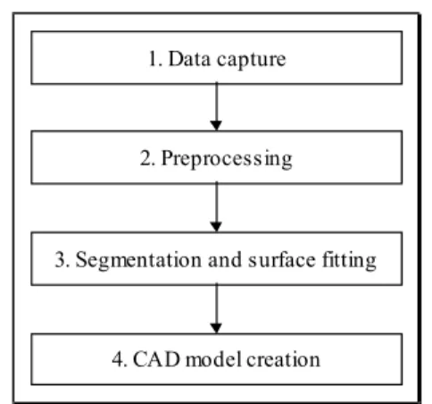
In many areas of industry, it is necessary to create geometric models of existing objects to allow an engineer to perform numerical simulations on these models. The reverse engineering process of digitized objects can be summarized by the flowchart of the Figure 1.
First of all, a set of 3D points is captured from the shape of the existing object. This digitizing process incorporates noise in the data and generally produces large sets of points, especially when laser sensors are used.
Secondly, the data can be pre-processed to perform data reduction and further noise reduction treatments. To this end, a mesh generation process is applied on the set of points to build a polyhedral model of the surface. Then, to reduce the noise and the amount of data, this polyhedron can be simplified. Among the main algorithms which are able to generate a mesh from a set of points, the « marching cubes » algorithm developed by Lorensen [Lorensen et al. 87] or the algorithm developed by Boissonnat [Boissonnat 88] dedicated to the meshing of parallel sets of points are examples of such mesh generation techniques. Algorithms for simplification will be dealt with later when presenting the preparation phases of the segmentation process.
At the third step, either the set of points or the polyhedron has to be segmented and then fitted with parametric surfaces to fulfill functional constraints. At present, various methods have been proposed. Among the most automatic methods, one is based on an arbitrary surface segmentation [Eck et al. 96], [Guo 97]. The patch decomposition is produced by simplification of an underlying triangulation that constitutes a particular parameterization of the final surface. However, this approach produces a patch decomposition that cannot reflect the functional structure of the shape, i.e. sharp lines and areas of rapid changes of curvature cannot be accurately restored. An efficient approach from an engineering point of view is based on a curve network that subdivides the surface by means of a set of characteristic curves (sharp edges, curvature discontinuity lines or lines where the curvature variation is maximum, symmetry lines, etc.). The objective of the current approach is to provide such
an appropriate engineering decomposition of a shape. Other approaches are based on point sets based on planar polygonal lines [Pizzi et al. 99] to extract feature lines used as basis of a segmentation process. Such a process is dependent on the sensor technology and the scanning technique and cannot be readily applied to configurations where an object must be scanned using several viewpoints. The proposed approach uses as input an unstructured polyhedral model that can be obtained from any technology of sensor and scanning technique.
Finally, a geometric model can be created from the set of parametric surfaces using form adjustments and blending functions.
4. CAD model creation 3. Segmentation and surface fitting
2. Preprocessing 1. Data capture
Figure 1: The main phases of a reverse engineering process.
The curve network previously mentioned cannot be automatically defined without local data about the surface curvature. Different approximations of gaussian and mean curvatures of a smooth surface approximated by a set of points or by a triangulation have been proposed [Lin et al. 82], [Stokely et al. 92], [Bahi et al. 95], [Martin 98] and [Boix 95]. Among these approximations, the last cited [Boix 95] owns some properties of convergence and form the basis of the criteria developed in the section 3. The use of local curvature criteria associated with different preparation processes enables interactive algorithms to define a first segmentation of the surface based on the identification of sharp lines (characteristic lines) and slow varying curvature areas (characteristic surfaces). The characteristic surfaces designate polygonal areas in the present context where the geometric model of the object is in fact a polyhedron. This segmentation will have to be processed further to obtain a set of partitions, which could be transformed through interpolation and/or smoothing algorithms into parametric surfaces. Such processes are necessary because this approach does not ensure that each partition has four borderlines. This post-processing and the interpolation and/or smoothing phase are out of the scope of the present document.
The segmentation approach presented here aims at introducing the interest of using different curvature approximations of a polyhedral surface to extract some of its geometric features. First of all, the task flow of the segmentation process is presented in the next section. Then, the discrete curvature approximations and invariant quantities are presented in section 3. The different treatments that prepare the polyhedral surface will be described at section 4. Then, the main concepts of the data structures set up are described at section 5. The basic concepts and principles of the line extraction and polyhedron segmentation are described as well as the algorithms set up to perform these tasks at sections 6 and 7 respectively. To conclude, some industrial examples of segmentation will illustrate the behavior of such criteria in the context of the segmentation process of digitized free form surfaces.
2. The segmentation approach
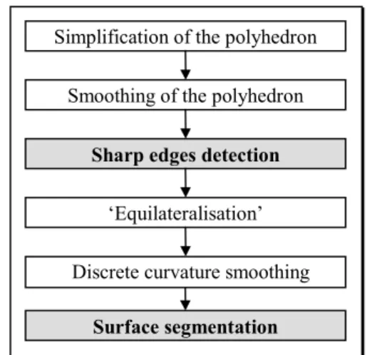
The approach proposed is based on different interactive phases to extract sets of polygonal lines and areas from the polyhedral surface in order to form partitions. Before each phase, a specific treatment optimizes the topological configuration of the polyhedron with respect to different criteria (Figure 2). Then, sharp edges (polygonal lines) are extracted, followed by the segmentation phase forming altogether a first segmentation of the surface.
The input data are assumed to come from a digitization phase of a three-dimensional object. Even if a noise reduction treatment has taken place during the digitization phase, the polyhedral surface still incorporates a fair amount of noisy and not significant data.
Thus, the first treatment consists in a simplification of this polyhedron (see section 4.1). The basic concept of the simplification process set up is to find a minimum polyhedron, i.e. a polyhedron with a minimum number of vertices and faces, with respect to several geometric and topologic criteria. A first criterion ensures that the
simplified polyhedron defines a surface located within a user-defined distance of the initial polyhedron [Véron et
al. 97]. A vertex removal technique forms the kernel of the process, similarly to other simplification methods
[Hoppe 96], [Puppo et al. 97]. However, the current approach is among the few that preserves the polyhedron conformity and restores as much as possible the shape of the object. Ensuring that the decimated polyhedron lies within a geometric envelope around the initial polyhedron is critical for the context of reverse engineering. In addition, the decimation process has a smoothing effect that reduces the measuring noise. To obtain an efficient smoothing effect it is highly necessary to avoid using control parameters based on angles between faces because these parameters can be hardly estimated by the user. When using angles, the decimated polyhedron tends to preserve wiggly areas that are not meaningful for the segmentation process.
Surface segmentation Sharp edges detection Smoothing of the polyhedron Simplification of the polyhedron
Discrete curvature smoothing ‘Equilateralisation’
Figure 2: The main phases of the segmentation approach.
To this end, different remeshing schemes are used during the simplification process. These schemes produce also a smoothing effect, i.e. the polyhedral surface is a better approximation of the real surface than the initial polyhedron [Véron 97], [Véron et al. 98]. This process is very important to correct mesh undulations in the neighborhood of sharp lines. To improve the approximation of some geometric quantities, the previous process is completed by a smoothing process based on a constrained edge-swapping operator applied on the polyhedron (see section 4.2). This constrained edge-swapping operator preserves the meaning of the resulting polyhedral surface since this surface still lies within the distance specified by the user. At the difference of other decimation schemes [Hoppe 96], [Puppo et al. 97], the one set up does not use angle parameters to leave the smoothing effect unbounded and produce a more intuitive user interface.
Then, sharp lines can be identified using an invariant criterion (see section 6). This means that this criterion is constant for equivalent meshes, i.e. meshes having different connectivities but describing the same geometry. The sharp lines identification is very important for the construction of a parametric surface because they locate G0 continuity areas between adjacent patches and form complementary constraints for the surface segmentation algorithm.
Afterwards, the surface has to be prepared for the surface segmentation process. Since the algorithm is based on discrete curvature approximations, the best result will be obtained when these approximations are the most accurate, i.e. when the polyhedron has the most equilateral faces as possible. In this case, it is not required that the curvature values must be meaningful with respect an equivalent smooth surface, it is only needed to obtain values around vertices that are meaningful with respect to each other. The fourth phase improves the mesh of the surface in accordance to this property (see section 4.3) and the fifth one performs a discrete curvature smoothing operation to reduce the side effects produced by the above local treatments (see section 4.4). Then, the user can split the surface apart to obtain adjacent areas. The results of the surface segmentation algorithm are sets of faces with an almost constant curvature (see section 7). Finally, each of these sets has to be processed to get a set of partitions such that none of them has more than four borderlines.
From each partition, a parametric surface patch can be fitted using smoothing functions for example.
3. Geometric criteria
A polyhedron is a piecewise linear representation of a smooth continuous surface which does not provide access to second order parameters like curvatures. In the scope of many applications however, obtaining local curvature values is important. To this end, different formulations of curvature or principal curvature approximations have been suggested [Stokely et al. 92], [Lin et al. 82], [Boix 95] and [Martin 98]. Some of them are curvature approximations formulated for sets of points. In this case, the computation of the curvatures is obtained after a
first approximation of the surface with a C² mathematical model like an ellipsoid. This way, the overall error attached to one digitized point, i.e. the manufacturing error of the mock-up, the digitizing error, is unevenly spread among the successive approximations (curvature approximations, further geometric approximations for the surface segmentation and sharp lines extraction) using different norms or measures. As a result, decision-making during an algorithm flow may not be adequate. In addition, if the vertex considered lies on a sharp line or at the intersection of sharp lines, using an associated continuous surface may lead to values identical to smooth areas leading difficulties when using a sharp line identification algorithm based on such quantities. If a polyhedron is used, the neighborhood of a vertex and an approximation of a whole surface are readily available and errors can be still modeled at each digitized point. Thus, a geometric approximation using a C2 surface, with
all its difficulties (undesirable local density of vertices, choice of the mathematical model, …) has not been retained. For these reasons, discrete curvature formulations based on polyhedron model have been preferred in order to provide quantities that enable the relative comparison of configurations of faces around a vertex.
The discrete curvature approximations at a point forming the basis of the geometric criteria are introduced. The convergence of the discrete gaussian curvature approximation towards the gaussian curvature of a C² surface passing through the same vertices has been proven by Boix [Boix 95], which is a complementary and useful property. The expression of the discrete mean curvature at an edge is based on the same work though no convergence property has been demonstrated yet. The discrete absolute curvature is obtained from the combination of both previous curvatures. Discrete invariant curvature criteria are invariant quantities of the previous criteria with respect to equivalent meshes. Hence, they intrinsically describe the local form of the surface around an edge or a vertex with regard to geometric concepts.
3.1. Discrete gaussian curvature
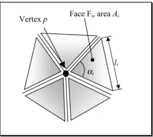
Often [Lin et al. 82], the discrete gaussian curvature Kp of a triangulation at a vertex p (Figure 3) is defined as the
ratio of the angle deviation at p to the area of the star-set attached to p:
∑
∑
− = i i i i p A K 3 1 2π α (1)where Ai is the area of the ith face connected at vertex p and αi the angle of this face at p.
This first approximation leads to a good approximation as long as the faces of the polyhedron are quite regular, i.e. all the faces have similar areas and are nearly equilateral. Boix [Boix 95] has proposed a new formulation. It is based on the modulus of a star-set that is quite different from the area of the star-set used in eq. (1) and gives eq. (2). It produces a better approximation of the gaussian curvature in most of the cases, mainly when faces have irregular areas and aspect ratios:
∑
∑
∑
− − = i i i i i i i p l A K 2 ). cot( 8 1 2 1 2 α α π (2)where Ai is the area of the ith face connected at vertex p, αi the angle of this face at p and li is the length of the
edge opposite to p.
Face Fi, area Ai
li
Vertex p
αi
Figure 3: Geometric parameters of a star-set associated to a vertex p.
More than an approximation of a value of curvature, the discrete gaussian curvature provides also information about the local form of the surface. Indeed, a positive value indicates that the surface is locally rather
spherical (Figure 4a), a null1 value points out that the surface is locally equivalent to a developable surface
(Figure 4b, 4c) and a negative value shows that the surface is locally like a pass (Figure 4d).
(b)
(a) (c) (d)
Figure 4: Geometric configurations of a surface according to its gaussian curvature.
3.2. Discrete mean curvature
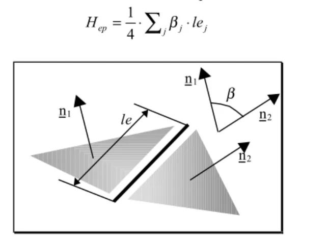
The discrete mean curvature He is basically defined for an edge [Bousquet 96] by eq. (3): e
e l
H = ⋅β⋅ 2
1 (3)
where le is the length of the edge and β the exterior angle between the normal of the faces adjacent at the current
edge (see Figure 5).
Assuming that He is uniformly spread along the edge, the discrete mean curvature can be evaluated at a
vertex p according to equation (4). The value of Hep around p incorporates the half sum of the value He of the
edges around the vertex p and enables the definition of cuvature quantities at the same location, i.e. at a vertex:
∑
⋅ ⋅ = j j j ep le H β 4 1 (4) le n2 n1 β n2 n1Figure 5: Geometric parameters used to define the mean curvature approximation along an edge.
To get a value of the discrete mean curvature at a vertex p, Hp, such that this approximation takes into
account the non uniformity of the triangulation, the value Hep of equation (4) can be divided either by the area of
the star-set (Eq. 5) or by the modulus of the same star-set attached to p (Eq. 6) to extend the proposals of Lin et al [Lin et al. 82] and Boix [Boix 95] with:
∑
∑
⋅ ⋅ = i i j j j p A le H 3 1 4 1 β (5)∑
∑
∑
− ⋅ ⋅ = i i i i i j j j p l A le H 2 ) cot( 8 1 2 1 4 1 α β (6) As it can be seen, the denominator of eq. (6) is identical to that of the best gaussian approximation one. Thetests carried out have shown that eq. (6) tends to produce the best mean curvature approximation though no convergence property could have been demonstrated yet. The important point being that eq. (6) provides values that are less sensitive to the aspect ratio of the star-set around a vertex and the values obtained are closer to mean
1 It is impossible to obtain a null value of the gaussian curvature due to the digitization noise, the numerical
roundoff errors, etc. This configuration is regarded as an idealized version of a range of configurations that are close to it within the measurin error.
curvature values associated to the C² surface built on polyhedron vertices as depicted by table 1. The tests performed showed that eq. (6) provides better results than eq. (5) in configurations where the polyhedron is close to a sphere, i.e. when the principal radii of curvature are close to each other. Since eq. (6) appears globally better than eq. (5) even though configuration (d) of figure 7 provided better results with eq. (5), eq. (6) has been preferred. No tests have been performed on cylinders approximated by triangulations since the decimation process that take place first on the digitized data to remove the measuring noise does not leave vertices along the generatrices of the cylinder apart from the extreme points defining the extremities of the cylinder (see section 4.1). At such vertices either the surface describes a half disk or it is adjacent to some other surface, hence comparing the values of discrete curvatures with curvatures over a smooth surface is no longer applicable. To avoid these configurations the decimation process uses specific remeshing schemes [Véron et al. 98] around the vertex removed.
(a) (b) (c)
(d) (e) (f)
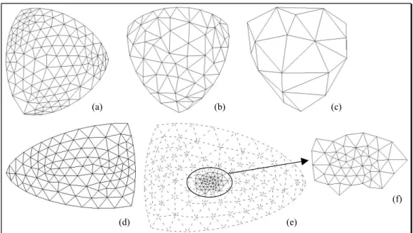
Figure 6: Various meshes of areas of spheres used for the computation of discrete mean curvatures using eq. (5) and eq. (6). (a) initial sphere of radius 1, (b) same sphere decimated with error zones of radius 0.01 (see section 4.1), (c) same sphere decimated with error zones of radius 0.05, (d) initial spherical area of radius 100, (e) initial spherical area after a mesh refinement operation,
(f) subset of (e) where the enriched area has been extracted.
Like the gaussian curvature, the discrete mean curvature contributes to give some clue about the local form of a surface. The local concavity (resp. convexity) of a surface is characterized by the sign of the mean curvature. Since this criterion is the average of both principal curvatures, its sign is the sign of the prominent curvature. Hence, three types of surfaces can be identified:
• convex surfaces where Hp is positive (Figure 8a), for example a ridge or a hill,
• ‘minimal’ surfaces1 (Figure 8b), for example a plane or a pass,
• concave surfaces where Hp is negative (Figure 8c), for example a valley or a hole.
3.3. Discrete absolute curvature
The absolute curvature Kabs at a point of a C² surface is defined as the sum of the squared principal curvatures
(Eq. 7). A combination of the mean and the gaussian curvatures produces also the same quantity. This criterion forms the basis of the sharp line detection algorithm because it gives an unambiguous characterization of a triangulation around a vertex p (see Figure 9 where characteristic lines are highlighted on the map).
K H k k
Kabs= 12+ 22=4 2−2 (7)
Hence, the discrete absolute curvature at a vertex p of a triangulation is defined by:
p p p abs H K K 4 2 2 − = (8)
1 Similarly to the gaussian curvature, a null value has to be interpreted as an idealized configuration of a
(a)
(b)
(c)
(e) (d)
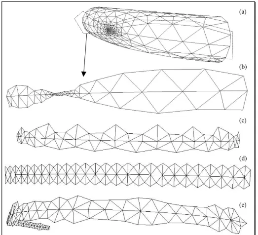
Figure 7: Various meshes of tori used for the computation of discrete mean curvatures using eq. (5) and eq. (6). (a) initial torus of external radius 100 and small radius 10, (b) detailed area along the external diameter of (a) where the discrete curvatures are computed, (c) area along the external diameter of a torus of external radius 170 and small radius 50, (d) area along the internal diameter of a torus of internal radius 100 and small radius 50, (e) area along the internal diameter of a torus of internal radius 50
and small radius 50. Type of test surface
according to figure 6
Discrete mean curvature computed with eq. (5)
Discrete mean curvature computed with eq. (6)
Mean value 1.03125627 1.00209009 Percentage of error 3.125 0.209 a Value computed on the
underlying sphere: 1.0
Number of points: 98
Standard deviation 0.01283894 0.00488273 Mean value 1.05482239 1.00695180 Percentage of error 5.482 0.695 b Value computed on the
underlying sphere: 1.0
Number of points: 38
Standard deviation 0.00528724 0.00319889 Mean value 1.20790933 1.03014177 Percentage of error 20.79 3.014 c Value computed on the
underlying sphere: 1.0
Number of points: 8
Standard deviation 0.10671866 0.00312529 Mean value 0.01027948 0.01001499 Percentage of error 2.794 0.149 d Value computed on the
underlying sphere: 0.01
Number of points: 72
Standard deviation 0.00067830 0.00000363 Mean value 0.01073797 0.01000674 Percentage of error 7.379 0.0673 f Value computed on the
underlying sphere: 0.01
Number of points: 30
Standard deviation 0.00001240 0.00002645
Type of test surface according to figure 7
Discrete mean curvature computed with eq. (5)
Discrete mean curvature computed with eq. (6)
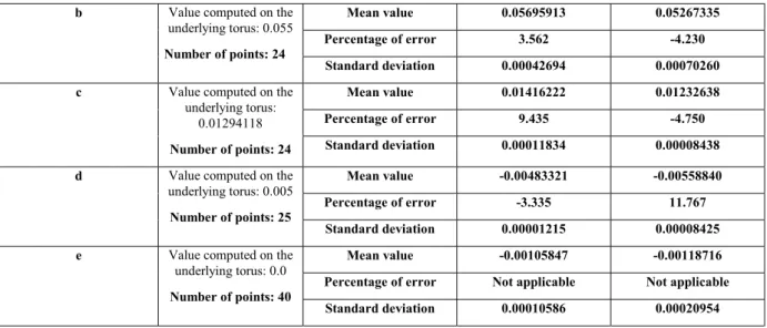
Mean value 0.05695913 0.05267335 Percentage of error 3.562 -4.230 b Value computed on the
underlying torus: 0.055
Number of points: 24
Standard deviation 0.00042694 0.00070260 Mean value 0.01416222 0.01232638 Percentage of error 9.435 -4.750 c Value computed on the
underlying torus: 0.01294118
Number of points: 24 Standard deviation 0.00011834 0.00008438 Mean value -0.00483321 -0.00558840 Percentage of error -3.335 11.767 d Value computed on the
underlying torus: 0.005
Number of points: 25
Standard deviation 0.00001215 0.00008425 Mean value -0.00105847 -0.00118716 Percentage of error Not applicable Not applicable e Value computed on the
underlying torus: 0.0
Number of points: 40
Standard deviation 0.00010586 0.00020954 Table 1: Comparison of discrete mean curvature values at a vertex using eq. (5) and eq. (6) on a sphere and along the main
diameter of a torus approximated by polyhedrons.
(a) (b) (c)
n n n
n n
n
Figure 8: Local concavity (resp. convexity) of a surface.
(a) (b)
Figure 9: (a) a polyhedron, (b) its map of the discrete absolute curvatures. The variation in the discrete absolute curvatures is due to the variations of the accuracy of the approximation errors and the irregularities over the mesh. Red areas indicate high
curvature values, black ones designates areas where the discrete absolute curvature vanishes and greenish ones indicates intermediate values.
3.4. Invariant criteria based on discrete curvatures
The discrete curvatures values are local approximations, which are meaningful in areas where a C² surface can be defined. At vertices lying on sharp lines, the value of discrete curvatures is no longer meaningful. In addition, the algorithm of sharp line identification comes after a constrained edge swapping algorithm, which smoothes the polyhedron. After this algorithm, the faces located near the sharp lines are generally thin and long. Therefore, the algorithm of sharp line detection needs to be based on criteria that do not depend on the mesh connectivity and on the shape of its faces but rely as much as possible on the form of the smooth surface that has been digitized. For example, the value of geometric criteria has to be the same for different meshes (Figure 10a, b, c) of the same geometric surface. Figure 10a, b, c depicts three equivalent meshes around vertex p. These meshes are said
equivalent because the faces connected at p change of size, their number changes also but they still represent locally the same corner of a box, i.e. they represent the same surface.
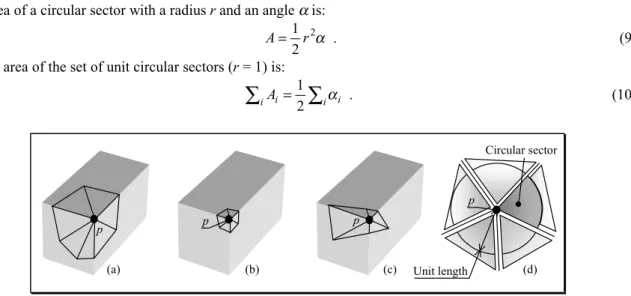
The objective is to replace the star-set at p by a set of unit circular sectors (Figure 10d). Thus, the area of the star-set reduces to the half sum of the sector angles (Eq. 10).
The area of a circular sector with a radius r and an angle α is:
α 2 2 1r
A= . (9)
So, the area of the set of unit circular sectors (r = 1) is:
∑
∑
iAi= 2 iαi 1 . (10) Unit length Circular sector (b) (c) (a) (d) p p p pFigure 10: (a,b,c) the same geometry at vertex p is described by equivalent meshes, (d) circular sectors associated to the star-set of the vertex p.
Using this transformation, the new criteria for the sharp lines detection algorithm are invariant for equivalent meshes and are expressed as:
• Invariant for the discrete mean curvature along an edge:
I
He=β, (11)Here, the concept of invariant is mainly characterized by the use of a unit length, • Invariant for the discrete mean curvature at a vertex p:
∑
∑
⋅ = i i j j p HI
α β 2 3 , (12)obtained from eq. (5). Similarly, another expression of
I
Hpcan be obtained from eq. (6).• Invariant for the discrete gaussian curvature at a vertex p:
( )
∑
∑
∑
⋅ − − = i i i i i i i p KI
α α α α π cot 8 1 4 1 2 2 , (13) • Invariant for the discrete absolute curvature at a vertex p:I
Kabs p 4I
Hp 2I
Kp2
−
= . (14)
The invariant for the discrete mean curvature (Eq. 12) is based on eq. (5) rather than eq. (6) since it produced better results (see Table 2). This is justified using the following tests. The quantity
I
Kabs p can beevaluated in four different ways using the two possible denominators for each quantity
I
Kp andI
Hp. If1
p H
I
is computed according to eq. (12),I
Hp2 is computed according to a denominator similar to that of eq.(13),
I
Kp1 is computed according to eq. (13),I
Kp2 is computed according to a denominator similar to that ofeq. (12), than four different quantities can be compared to define the
I
Kabs p parameter, i.e.:1 2 1 1 4 p 2 p p abs H K K
I
I
I
= − , 1 2 2 2 4 p 2 p p abs H K KI
I
I
= − , 2 2 1 3 4 p 2 p p abs H K KI
I
I
= − , 2 2 2 4 4 p 2 p p abs H K KI
I
I
= − .The different values of
I
Kabs p need not be compared with a reference value computed on a smooth surfacesmooth. Two comparisons are performed in configurations where ‘principal curvatures’ are assumed as equal and when there are finite though different from each other. In the first case, the error measured is given by:
(
)
100 1 ,[ ]
1,2 100 2 2 ∈ − × = − × = j K H K H K E pj pj pj pj pj iI
I
I
I
I
, (15)to express the deviation of
I
Hpjwith respect toI
Kpj. In the second case, assuming the ‘principal curvatures’satisfy: x=k1 k2 and x is known if the polyhedron lies on a known torus, than eq. (15) becomes:
[ ]
1,2 , ) 1 ( 4 1 100 2 2 ∈ + − × = j K x H x E pj pj iI
I
. (16)Using eq. (15) and (16), table 2 provides the comparisons based on the polyhedrons displayed on figures 6 and 7. As stated above, the error E tends to be the smallest for the tests performed. Therefore, 1
I
Kabs p1 can beconsidered as the most appropriate expression of
I
Kabs p.4. Pre-treatments
For each pre-treatment, the aim of the algorithm will be presented. Then, the algorithm principle will be described. To conclude, some results of each pre-treatment as well as its contribution to the segmentation approach will be provided.
4.1. Simplification process
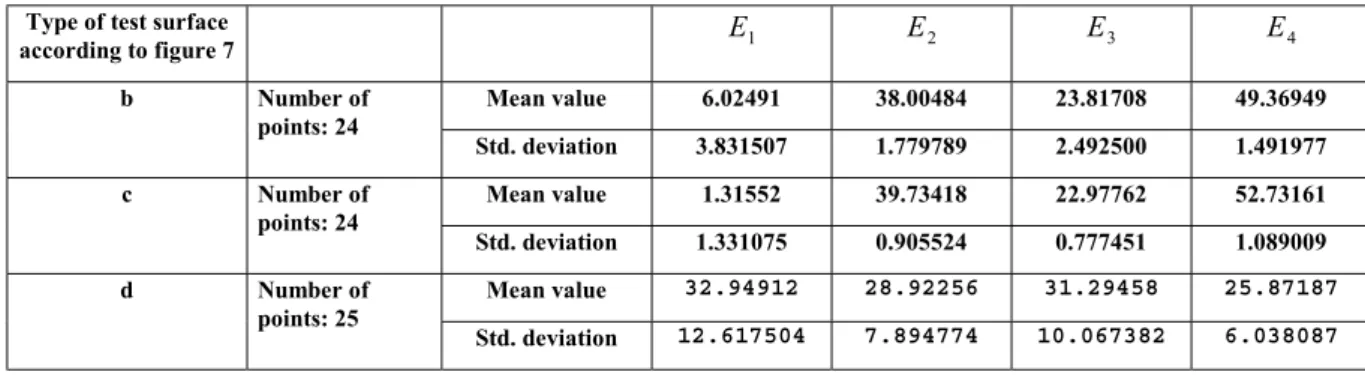
The aim of this treatment is to reduce the amount of data and the associated noise [Véron et al. 97], [Véron et al. 98]. Indeed, digitizing devices can produce large amounts of noisy 3D points leading the polyhedral representation of objects to a treatment of simplification, which improves the segmentation process. In figure 11, the initial polyhedron (a) is defined with 11 730 vertices and 23 379 faces while the dimensions of the object are 108 x 104 x 21 mm. With an error zone equal to 0.01 mm (the error zone concept will be defined later, but to give an idea, the error zone has the same order of magnitude than the measuring accuracy of the 3D sensor), the simplified polyhedron (b) is reduced to 5 266 vertices and 10 451 faces. The amount of data has been divided by two and the surface is less noisy.
Type of test surface
according to figure 6 E1 E2 E3 E4 Mean value 1.80083 20.10652 12.06543 26.61895 a Number of points: 98 Std. deviation 3.836446 0.632055 1.593659 0.912970 Mean value -14.94345 22.26747 6.96706 33.34166 b Number of points: 38 Std. deviation 5.295912 1.303506 1.218364 2.593458 Mean value -55.36201 27.32936 -3.48373 46.38765 c Number of points: 8 Std. deviation 19.979185 3.504346 5.224393 6.262015 Mean value 6.00543 21.17745 14.17433 27.24444 d Number of points: 72 Std. deviation 1.385087 0.412006 0.405738 0.921698 Mean value 1.47744 21.78089 12.84512 28.89709 f Number of points: 30 Std. deviation 3.115565 1.109449 0.704243 2.347589
Type of test surface according to figure 7 E1 E2 E3 E4 Mean value 6.02491 38.00484 23.81708 49.36949 b Number of points: 24 Std. deviation 3.831507 1.779789 2.492500 1.491977 Mean value 1.31552 39.73418 22.97762 52.73161 c Number of points: 24 Std. deviation 1.331075 0.905524 0.777451 1.089009 Mean value 32.94912 28.92256 31.29458 25.87187 d Number of points: 25 Std. deviation 12.617504 7.894774 10.067382 6.038087 Table 2: Comparison of invariants of discrete mean curvature values at a vertex using eq. (5) and eq. (6) on a sphere and along the
main diameter of a torus approximated by polyhedrons.
(a) (b)
Figure 11: Simplification of a polyhedral model of a part of a ski boot mould (courtesy Fidia-KMR) (a) initial polyhedron, (b) simplified one.
The interest of this algorithm resides in the continuous control of the polyhedron geometry during the simplification process. Indeed, the user chooses the sizes of the error zones. These zones are spheres, with a predefined radius, centered at each vertex of the initial polyhedron. The set of spheres acts like a discrete envelope around the initial polyhedron that bounds the deviation of the simplified polyhedron with respect to the initial one. Then, the algorithm ensures that the simplified polyhedron intersects each of them. This restoration control concept allows the algorithm to keep the simplified polyhedron included into a geometric envelope defined by all the error zones attached to the initial model. This principle of geometric control is illustrated in figure 12 for vertices lying on the polyhedron boundaries. A similar concept is applied to vertices lying into the domain represented by the polyhedron surface. An inheritance process of error zones attached to faces helps transfer the error zones during the vertex removal process. The vertices are selected for removal according to the increasing values of Kabs pto produce a smoothing effect and hence, remove the measuring noise.
This algorithm allows the polyhedron to exhibit sharp lines. However, this treatment tends to remove all the vertices located on planar or cylindrical areas but avoid those located at their boundaries. As a result, the discrete curvature approximations are no longer meaningful (see Figure 13) and cannot be used to perform the polyhedron segmentation. To prevent from such a behavior, the simplification algorithm incorporates another criterion to leave some vertices on plane and cylindrical areas. When a vertex is simplified, if one of the new edges created by a remeshing scheme is longer than a threshold value, the simplification is not allowed. This criterion reduces the number of vertices removed but generates a representation of the surface through a rather regular mesh and produces useful curvature approximations. Depending on the characteristic information looked for, either of the previous decimation schemes may be of interest. The last one is especially of interest when segmenting the polyhedron for polyhedral surface areas.
Error zone
(a) Simplification allowed (b) Simplification not allowed
Initial polyhedron
Geometric envelope
Figure 12: Principle of the simplification algorithm, the simplified polyhedron does not intersect each of the error zones (b) whereas it does (a)
Figure 13: Simplification of a polyhedron with a small dimension of error zone. The vertices on the spherical surface have not been simplified but the vertices lying on cylindrical or plane surfaces have all been simplified.
4.2. Smoothing process
The aim of this treatment is to smooth the polyhedron in order to improve the mesh connectivity near the sharp lines. The simplification algorithms are based on vertex selection criteria that rely on local characteristics (Kabs p) and hence do not allow it to trace the sharp edges. In addition, the sequential vertex removal process
does not favor an efficient preservation of the sharp lines across the successive remeshing phases taking place each time a vertex is removed. As a consequence, the sharp lines are not entirely discretized as polygonal lines in the simplified polyhedron. The Figure 14 illustrates this configuration and shows the result of the constrained edge-swapping algorithm.
(a) (b)
Figure 14: Detail of a polyhedral surface before (a) and after (b) the smoothing algorithm.
The smoothing algorithm consists in minimizing a cost function using an edge-swapping operator. This operator is iteratively applied to each edge of the simplified polyhedron and the geometry restoration control (the
same as for the simplification algorithm) is also active, i.e. §4.1: the new faces must intersect the error zones that were initially attached to the faces before the edge swapping operation. The cost function Fma (Eqs. 17 & 18) is
defined as the sum of the angles formed by the faces F1 and F2 and their adjacent faces (Figure 15), i.e. the sum of
the invariant discrete mean curvature (
I
He) of each edge of both faces. This function is computed before and after each edge swapping operation. After the edge swapping operation, if the cost function is less than before and if the restitution criterion (intersection between all the error zones attached to faces F1 and F2 and the faces F’1 andF’2) is validated, the polyhedron is modified. This operator is applied to each edge of the polyhedron until no
other edge can be swapped. Though the combination of the cost function and the geometric restoration control do not enforce the convergence of this process, no significant negative effect of lack of convergence has been noticed concerning the improvement process of the sharp line discretization.
F’1 F’2 E’ n'1 n'2 n3 n4 n6 n5 E F1 F2 n1 n2 n3 n4 n6 n5 (b) (a)
Figure 15: Parameters used by the Fmacost function before (a) and after (b) the edge swapping.
Initial cost function: Fma =β(n1,n2)+β(n1,n3)+β(n1,n4)+β(n2,n5)+β(n2,n6) (17)
After the edge swapping: Fma'=β(n'1,n2)+β(n'1,n3)+β(n'1,n6)+β(n'2,n4)+β(n'2,n5) (18)
where (ni, nj) is the exterior angle between the normal ni and nj of the faces Fi and Fj (see Figure 15). 4.3. ‘Equilateralization’ process
As soon as the sharp edges have been identified with a line extraction algorithm (see figure 2), the mesh of the polyhedron has to be optimized with respect to the discrete curvature approximations. The best approximation results are obtained when the faces of a star-set at a vertex p are close to equilaterality as depicted by Boix [Boix 95]. Indeed, it does not seem adequate to retriangulate the polyhedron using a new set of vertices since a reduction of the number of vertices is not acceptable from the noise reduction point of view, i.e. a decimation process has already produced a polyhedron as close as possible to the envelope of measuring noise. At the opposite, increasing the number of vertices must not generate noise and should not be computationally expensive. Thus, the idea is to get closer to this configuration using an edge-swapping operator based on a specific cost function (Eq. 19). The cost function Fe is defined as the largest angle αi at each vertex of the faces F1 and F2
(Figure 16). ) max min( min 6 1 i i i e F = α = = (19) F2 F1 α1 α2 α4 α5 α6 F’2 F’1 (b) (a) α3 α1 α2 α3 α4 α5 α6
Figure 16: Parameters used by the Fe cost function before (a) and after (b) the edge swapping.
This ‘equilateralization’ process is repeatedly applied to the edges of the mesh. However, the edges taking part to the polylines describing the sharp edges are not subjected to this treatment. Though the convergence of
this algorithm does not exist from a theoretical point of view, the improvement of the discrete curvature approximations has not highlighted an influence of this lack of property. In addition, like the previous edge swapping operator this edge-swapping operator is also associated to the geometric restoration control criterion. Using this process, the discrete curvature approximations are significantly improved over the simplified polyhedron as illustrated on figure 17, where the tessellation obtained (b) provides more equilateral faces, though the resulting polyhedron still lies within the envelope characterizing the measurement noise.
(a) (b)
Figure 17: Influence of the ‘equilateralization’ process. (a) simplified polyhedron. (b) polyhedron simplified with an edge length criterion and obtained after the ‘equilateralization’ process.
4.4. Discrete curvature smoothing
Though the previous treatments are efficient, the noise and the mesh connectivity cannot be adequate everywhere. Indeed, the noise is not evenly distributed over the polyhedron and some significant edges can be missing due to the digitization process. Small details, as well as the technology of the sensor and digitizing system often are not producing reliable digitized models where some feature edges of the model don’t exist in the polyhedron. Therefore, the discrete curvature approximations produced by the ‘equilateralization’ process can hardly be incorporated into a surface segmentation criterion.
On a smooth surface, the curvature variations are progressive, excepted along sharp lines and limits of blending areas. Based on this remark, the curvature approximation could be improved. Since the identification of characteristic areas relies on vertex-based approximations, a discrete curvature smoothing process can be performed on the values of Kp, Hp, Kabs p at each vertex that does not lies on a sharp line or on a boundary of the
polyhedron. Each of the discrete curvatures at a vertex Ni is defined as the weighted average of the curvature at
this vertex and of the curvature at its neighbor vertices. The farther a vertex Nj from the current vertex Ni, the less
significant its discrete curvature value. Hence, the weight wj assigned to each neighbor vertex is defined as:
j i j N N w = 1 (20)
The algorithm restricts the neighborhood of a vertex to an area of topologic radius of two vertices, i.e. the shortest path from the current vertex to a target vertex, measured in number of edges, defines the topologic radius between these two vertices (see figure 18). The neighborhood of a vertex is restricted to an area that does not include vertices located on a boundary or on a sharp line.
Sharp line edge
Vertices within a topologic radius of two vertices
Ni
Figure 18: Vertices within a topological radius of 2.
The figure 19 illustrates the effect of the smoothing process for a polyhedron. The color scale is similar to that of figure 9 previously used.
(a) (b)
IKabs p max
IKabs p min
Figure 19: Effect of the smoothing process: (a) initial discrete curvature map, (b) smoothed map.
5. Data structure
During the various phases, the algorithm identifies a set of partitions and their borderlines. The results are saved into two main data structures. The first one, which is called “boundary”, contains a set of ordered boundary edges. The second one, which is called “partition”, contains a set of faces and a set of boundaries. A “boundary” defines a borderline of a “partition”, such that it intersects another “boundary” only at its extremities to form a pattern on the polyhedron.
A classification of the edges, the vertices and the boundaries is required for the algorithm and for the post-processing of the results. It is obtained with the following rules (see figures 20 and 21).
Classification of the edges:
• An edge of a boundary identified as a sharp edge of the polyhedron is classified as a “boundary edge”, • An edge of a partition is classified as a “partition edge” (all the edges that are not boundary edges are
partition edges).
Classification of the vertices:
• A vertex connected to one or two boundary edges only is classified as a “boundary vertex”, • A vertex connected only to partition edges is classified as a “partition vertex”,
• A vertex connected to two more than two boundary edges is classified as a “extremity vertex”.
partition vertex boundary vertex extremity vertex partition edge boundary edge
Figure 20: Classification of the edges and the vertices of a polyhedron for the segmentation process.
Classification of the boundaries:
• A boundary which defines a sharp edge is classified as a “C0 boundary”,
• A boundary connected to two partitions is classified as a “Gn boundary”, if it has not been classified as a “C0
boundary”,
• A boundary connected to one partition only is classified as a “undefined boundary”, if it has not been classified as a “C0 boundary”.
C0 boundary
Gn boundary
Figure 21: classification of the boundaries of a polyhedron.
The boundary classification helps create useful information to characterize the patch decomposition of a surface as far as it can be from a polyhedral representation. Gn continuity means that G1, G2, …, continuities
cannot be distinguished.
6. “Sharp lines” identification
The sharp edges of an object represented by a polyhedron are considered as privileged boundaries of patches. Indeed, from a practical point of view, Bézier patches cannot describe tangent plane discontinuities. Only NURBS patches can incorporate some tangent plane discontinuities. Whatever the model, the sharp edges have to be identified to generate tangent plane discontinuities either between two patches or within a NURBS patch. Hence, each curve identified with the next algorithm will be the boundary of two patches connected with a C0
continuity. This process takes place after the initial polyhedron has been simplified and the constrained edge-swapping operator has been applied. If the decimation process of the polyhedron takes place with an edge length threshold, it does not produce incompatibilities with the sharp line extraction process.
6.1. “Sharp lines” identification algorithm
The figure 22 presents the algorithm for extracting sharp lines from a polyhedral model of the object shape. The user monitors the result through a user-defined threshold value (TVIH). TVIH defines the minimal angle between
the adjacent faces separated by the sharp lines.
The update of the vertices and edges classifications is carried out at the end of each ‘Loop 1’. This classification is useful to easily identify each entity during the algorithm.
The edges describing a sharp line are stored in a structured list. At the end of the algorithm, the lists are processed to generate the C0 boundaries (Figure 22). Indeed, a boundary is defined as a list of connected edges
with only two extremity vertices located at its extremities. The edge lists identifying the ‘sharp lines’ frequently cross each other. Consequently, the sequences of edges obtained are processed to extract their boundaries, i.e. the extremity nodes where the sharp lines cross each other. This is achieved by looking for similar vertices numbers into two distinct edge lists. If such vertices appear, they are transformed into extremity vertices. Then, each edge list is scanned to extract each edge subset contained between two extremity vertices to form ‘sharp edges’ (see Figure 23).
6.2. Criteria for finding the candidate edge
The map of the invariant discrete absolute curvature “IKabsp” shows that the sharp lines of the object are located
in areas of high absolute curvature in comparison with their nearest neighborhood (Figure 24). Nevertheless, in the areas where many sharp lines are connected, there is a high density of vertices with high absolute curvature values (Figure 25: areas marked with a 7777). Thus, the “IKabsp” criterion is not meaningful enough because it is too
local since it is concentrated at a vertex (Figure 24a) and curvature information between two vertices is required. Indeed, an edge crossing a plane can have at its extremities two vertices with high curvature values. The invariant of the mean curvature of an edge, “IHep”, produces some complementary information (Figure 24b). So, a more
robust selection is obtained with multiple criteria to generate the widest point of view at a vertex (Figure 24c): a first selection of a given number of edges, α, extracts information from the edges connected at the current vertex using the “IHep” criterion and then, the candidate edge chosen within this resulting set is finally selected with the
“IKabs p” criterion evaluated at the vertices surrounding the current one. The corresponding pseudo-code is
provided below (Figure 26).
No
End of the sharp line extraction
No End of the algorithm Sort the vertices by decreasing values of IKabs p
Select the candidate vertex, i.e. the vertex with the highest value of IKabs p.
Is its value higher than the user threshold value ?
Find the candidate edge among those connected at the current vertex. (see section 6.2)
Is there a candidate edge?
The second extremity vertex of this edge becomes the current vertex.
Does it define
an extremity vertex of a boundary ? No Yes
End of the sharp line extraction. Yes
Loop 2
Loop 1 Yes
Update of the vertices and edges classifications
Figure 22: “Sharp lines” identification algorithm.
Extremity node 1st extremity node of
the set of edges.
Sets of edges 1st boundary generated n+1th boundary generated 2nd boundary generated (a) (b) nth boundary generated
Figure 23: (a) initial data: set of edges and extremity vertices; (b) subdivision of the initial edge lists to produce the final C0 boundaries.
used curvature unused curvature
a b c
Figure 24: Wider point of view obtained with complementary parameters.
7 77 7
IKabs p max
IKabs p min
Select α edges with the “IHep” highest value from the set of edges adjacent to the current vertex.
Keep only the edges having a “IHep” value higher than the first threshold value (TVIH).
Keep among the set of select edges, the edge with the highest “IKabs p” value at its second vertex.
If this “IKabs p” has a value higher than the second threshold value (TVIK),
Then the edge is the candidate edge, Else there is no other candidate edge.
Figure 26: Algorithm to find the candidate edge.
Sharp line edge
Ni
TVIH
Ni is an arbitrary point
along the sharp edge Disk used to characterize the invariant around Ni
Fictive and arbitrary edge around
Ni to define the invariant
Figure 27: Determination of the TVIK value from the user-defined TVIH value.
The TVIH threshold value is user-defined. This threshold is the minimal angle formed by the two faces
adjacent to a sharp line (see Figure 27). The TVIK value is then deduced using the concept of invariant (see
Figure 27). This threshold is the “IKabs p” value at an arbitrary vertex on a linear sharp edge where the “IHep” value of the edges on this sharp line is the TVIH value. Then, using the concept of invariant where Ni is an arbitrary
vertex on a sharp edge and any arbitrary triangulation is built around Ni on the two adjacent faces, TVIK can be
computed from TVIH using eq. (14). α is the parameter used for the multiple selection of edges around the current
vertex, the experimentation shows that α = 3 works well in most of the configurations. However, this parameter can be forced by the user when required.
6.3. Post-processing
The “sharp lines” identification algorithm cannot produce acceptable results in all cases. All polyhedrons are particular and a generic algorithm does not exist. Ideal polyhedrons, which come from a mesh of CAD models, do not necessarily need a post-processing phase. But for the polyhedrons that come from digitized data, the sharp lines are not all correctly identified because the algorithm generally finds a lot of parasite lines, or parallel lines defining the same characteristic line of the object shape or cannot identify all the bifurcations of sharp lines since the threshold values are constant over a given polyhedron during the identification process.
Therefore, few treatments have been developed to improve the previous results and allow the user to adapt the result to his (resp. her) interpretation because at present the constant threshold values do not allow to generate a robust process. Some of these processes are automatically executed after the algorithm and they correct most of the ‘wrong sharp edges’.
Generally, the user has to choose among various possibilities of the location of sharp edges or about the existence or not of such lines. Hence, few interactive treatments allow him (resp. her) to remove, recompute, …, the sharp lines selected [Lesage 98].
6.3.1. Automatic treatments
To improve the results of this algorithm, few automatic treatments are implemented:
• Sometimes, a sharp line of the real object can be identified as two or more polygonal ‘sharp lines’ as defined by the previous sections. Therefore, a specific treatment adjusts this result by searching these polygonal ‘sharp lines’ for those that have only one neighbor sharp line at their extremities and merges them together to produce automatically a more significant polygonal line,
• Into some configurations, the sharp lines can be badly defined because the constant values of the thresholds used over a whole polyhedron cannot be adequate everywhere. With such a context, the algorithm may define locally two different polygonal lines to represent the same sharp line, for example. Therefore, a treatment has been set up to look for parallel sharp that are close to each other and remove one of them.
• An isolated sharp line composed of few edges only can by defined when the polyhedron incorporates configurations that are slightly under the user-defined threshold. This specific treatment removes the small and standalone sharp lines according to a user-defined threshold value, i.e. the maximal length of the sharp lines to be removed.
6.3.2. Interactive treatments
Interactive treatments means that the user selects a set of sharp lines and applies the appropriate tool among the following:
• Removal of a set of selected sharp lines: despite of the greatest care to set threshold values, the algorithm frequently identifies sharp lines that are not of interest. Again, this behavior occurs because a constant threshold value over a whole polyhedron cannot incorporate the diversity of configurations found over a complex model. This problem appears particularly along blending surfaces which are poorly digitized and can lead the algorithm to interpret such areas as a location of sharp line,
• Sharp line extension: when the user has defined a too large threshold value, some sharp lines are not entirely identified. To correct this behavior, the user can extend independently each sharp line by changing the threshold value in real time in order to tune the threshold value to a locally adequate value, • Sharp lines merging: a sharp line can be divided into several pieces due to some defects on the initial
polyhedron because of imperfections in the model itself or because of the behavior of the sensor during the digitizing phase. Hence, the user can decide to merge together two sharp lines to correct such configurations that cannot be addressed by the segmentation algorithm.
7. Surface segmentation process
The main idea of the surface segmentation process is to break down the surface into a set of polyhedral areas or partitions, i.e. a partition is a connected set of faces, having a slowly varying discrete absolute curvature. Each of them is extracted using a frontal method after the identification of sharp lines has taken place. Faces adjacent to this front are added to the partition if the value of the discrete absolute curvature approximation for each of their vertices lies within the user-defined curvature limit values. Sharp lines as defined before, prescribe curvature or tangency discontinuities that form complementary constraints for the front propagation algorithm. The boundaries of the partitions define polygonal lines where the surface has a continuous variation of the tangent plane and a rapid change of curvature simultaneously, like boundaries of blending areas. This segmentation process helps providing a functional decomposition of the object and is based on the ‘equilateralization’ and the discrete curvature smoothing processes as pre-treatments before the surface segmentation itself.
7.1. Partition identification algorithm
As stated previously, the approximations of discrete curvatures are meaningful for polyhedrons with a good aspect ratio of the faces, i.e. the faces are close to equilaterality. However, polyhedrons may be described through a wide variety of meshes depending on the criteria used within the treatments producing the input mesh. As a result, a polyhedron with a high density of vertices will have to use the discrete absolute curvature criterion to perform the surface segmentation. With such an approximation, the evolution of the curvature over the surface has a better representation but when a polyhedron is represented with few vertices (a bit more than the polyhedron of the Figure 13, which has to be processed by another algorithm), the algorithm would have to use the invariant approximation of the discrete absolute curvature because the results are too poor with the first criterion since the faces of the polyhedron will never be able to be equilateral enough even after the use of the ‘equilateralization’ process. Such differences of configurations demonstrate the importance of the control of the edge length during the decimation process to produce a polyhedron better suited for the surface segmentation process.
This algorithm breaks down a polyhedral surface into a set of partitions. The user-defined interval of discrete absolute curvature, i.e. [Kabs m, Kabs M], enabling the vertices to be added to a partition is defined by two
threshold values, Kabs m and Kabs M. Thus, each partition is a portion of the polyhedral surface (a set of adjacent
faces) whose curvature lies within the interval defined by the user.
The initialization of a partition requires the selection of a first face. The discrete curvature at each vertex of such a face must lie within the user-specified interval of curvature. The first face found in the polyhedron that matches this criterion is selected to initiate a front. Each edge of this face initializes the set of boundary edges of the front (Figure 28a). Then, the adjacent face to each edge of the front boundary is candidate for the propagation. Each edge used is removed of the front boundary (Figure 28b). The faces that passed the test for insertion into the current partition are added to the front and their edges are classified. The edges that are not classified as “boundary edge” or “partition edge” are added to the front boundary (Figure 28c).
a b c y
n y
Has the face passed the test ? y (yes) or n (no) new partition
front boundary
boundary edge partition edge
Figure 28: Initialization and first iteration of the front propagation algorithm
At the end of this process, when all the faces of the polyhedron that do not already belong to partitions have been evaluated, new boundaries are built using the same method as for “C0 boundaries” described for the
identification of sharp edges. At this stage, the boundaries are associated with their respective partitions. Figure 29 summarizes the main steps of this front propagation process.
Prior to this front propagation process, the vertices of the polyhedron are sorted according to the decreasing values of Kabs in order to identify the candidate vertices that could initiate a partition. To this end, their Kabs value
is compared to the lower bound of the user-defined interval Kabs m.
No End of the algorithm Sort the vertices by decreasing values of Kabs.
Select the unprocessed vertex p with the highest Kabs value
Is its value greater than the user threshold value Kabs m ?
Select a face adjacent at the vertex p for which the two other vertices have values of Kabs ∈ [Kabs m, Kabs M]
Yes
Is there a face selected ? Yes
Loop 1
The edges of this face are saved in the front boundary.
For each edge of the front boundary, determine if the neighbor face is candidate. (each vertex of the face has to satisfy Kabs p ∈ [Kabs m, Kabs M])
Are there some faces selected? Yes
No End of the front
Update the type of the vertices, the edges and the candidate faces. Update the boundary front.
Is the boundary front empty ? Yes
No
End of the front
Loop 2
Non processed area Partition 1 Partition 3 Partition 2 B1 B2 B3 B4 B5 Partitions C0 boundary Gn boundary no def. boundary Extremity node
Figure 30: Illustration of the update process of boundary types according to the results of the segmentation process.
The figure 30 illustrates the update of the boundary type according to the results of the surface segmentation process:
• The boundaries “B1” and “B2” are both “C0 boundaries”; the first one is adjacent to “Partition 1” and
“Partition 3”, while the second is adjacent to “Partition 1” only,
• The boundaries “B3” and “B4” have one adjacent partition only; their type is therefore “undefined”,
• The boundary “B5” has two different adjacent partitions; it becomes a “Gn boundary ”.
As depicted in figure 30, the “C0 boundaries” are kept unchanged after the line segmentation process. The surface segmentation process produces only “Gn boundaries ” and “undefined” ones depending respectively on
the existence of one partition on both sides of the boundary or the presence of only one partition attached to the boundary. The sequential process of partition identification justifies the necessity of the “undefined” boundary status since the whole surface of the polyhedron cannot be covered at once, thus leaving some areas unprocessed and creating boundaries attached to one partition only. It is therefore not possible to characterize the class of the boundary.
7.2. Post-processing applied to the partitions
According to the user chosen thresholds, the segmentation can neither be improved everywhere nor correspond to the user’s expectations. Indeed, for some areas of the surface, the thresholds are not adequate (too small or too large values) or, according to the nature of the object processed and the amplitude of the measuring noise, many useless partitions can appear. Up to now, these configurations cannot be handled automatically. Hence, some interactive tools have been set up to allow the user to improve the first solution provided by the surface segmentation algorithm similarly to the boundary extraction process tools:
• Connect partitions: a new partition can be defined from two adjacent partitions. Both sets of faces and sets of boundaries are gathered. The common boundaries are removed and some boundaries are linked together if it is needed,
• Extend partitions: the user can extend a selected partition by changing interactively the threshold values. This algorithm defines a new boundary front from the “undefined” boundaries of the partition. Then, the loop 2 of the segmentation algorithm is performed. This treatment is especially dedicated to partitions incorporating “undefined” boundaries because if a partition does not involve such a partition it is pointless to try to extend it,
• Remove partitions: the user can remove selected partitions or the small partitions (partitions owning less than n user-defined elements). This particularly important either to remove small partitions or to allow the user to restart the segmentation of an area where the decomposition is not satisfactory,
• Smooth boundaries: the boundaries of partitions obtained tend to oscillate because the front propagation process is based on the existing faces. These faces are built from a subset of the digitized points; therefore the boundary of a partition cannot be smooth. In addition, pre-treatments such as the ‘equilateralization’ of faces increase this behavior. To improve, the quality of the partition boundary and ease the curve generation process that will take place afterwards, a smoothing algorithm, which can use an edge-swapping technique, is required. However, such a treatment has not been incorporated yet and the results presented on figures 31 and 32 are the direct output of the partition identification process.
8. Example of results
The line and surface segmentation algorithms described above have been applied to a digitized free-form surface representing a part of a ski boot mould (see also figure 11 for a wire frame representation of this surface). This model has been digitized with a mechanical sensor having an accuracy of 0.05 mm. The length of the subset considered is of 100 mm.
The magnitude of the accuracy of the sensor has been used to perform the decimation process with a diameter of the spheres of 0.05 mm.
![[PDF] Manuel complet du langage C++ pour les nuls | Cours informatique](data:image/gif;base64,R0lGODlhAQABAIAAAP///wAAACH5BAEAAAAALAAAAAABAAEAAAICRAEAOw==)