arXiv:1302.5119v1 [astro-ph.SR] 20 Feb 2013
April 8, 2013
Chemical surface inhomogeneities in late B-type stars with Hg and
Mn peculiarity
I. Spot evolution in HD 11753 on short and long time scales
⋆,⋆⋆H. Korhonen
1,2,3, J.F. Gonz´alez
4, M. Briquet
⋆⋆⋆5,6, M. Flores Soriano
7, S. Hubrig
7, I. Savanov
8, T. Hackman
3,9,
I.V. Ilyin
7, E. Eulaers
5, and W. Pessemier
61 Niels Bohr Institute, University of Copenhagen, Juliane Maries Vej 30, DK-2100 Copenhagen, Denmark
e-mail: heidi.korhonen@nbi.ku.dk
2 Centre for Star and Planet Formation, Natural History Museum of Denmark, University of Copenhagen, Øster Voldgade 5-7,
DK-1350 Copenhagen, Denmark
3 Finnish Centre for Astronomy with ESO (FINCA), University of Turku, V¨ais¨al¨antie 20, FI-21500 Piikki¨o, Finland 4 Instituto de Ciencias Astronomicas, de la Tierra, y del Espacio (ICATE), 5400 San Juan, Argentina
5 Institut d’Astrophysique et de G´eophysique, Universit´e de Li`ege, All´ee du 6 aoˆut 17, Sart-Tilman, Bˆat. B5C, 4000 Li`ege, Belgium 6 Instituut voor Sterrenkunde, Katholieke Universiteit Leuven, Celestijnenlaan 200 D, B-3001 Leuven, Belgium
7 Leibniz-Institut f¨ur Astrophysik Potsdam (AIP), An der Sternwarte 16, 14482 Potsdam, Germany 8 Institute of Astronomy, Russian Academy of Sciences, Pyatnitskaya 48, Moscow 119017, Russia 9 Department of Physics, PO Box 64, FI-00014 University of Helsinki, Finland
Received September 15, 1996; accepted March 16, 1997
ABSTRACT
Aims.Time series of high-resolution spectra of the late B-type star HD 11753 exhibiting HgMn chemical peculiarity are used to study the surface distribution of different chemical elements and their temporal evolution.
Methods.High-resolution and high signal-to-noise ratio spectra were obtained using the CORALIE spectrograph at La Silla in 2000, 2009, and 2010. Surface maps of Y ii, Sr ii, Ti ii, and Cr ii were calculated using the Doppler imaging technique. The results were also compared to equivalent width measurements. The evolution of chemical spots both on short and long time scales were investigated.
Results.We determine the binary orbit of HD 11753 and fine-tune the rotation period of the primary. The earlier discovered fast evolution of the chemical spots is confirmed by an analysis using both the chemical spot maps and equivalent width measurements. In addition, a long-term decrease in the overall Y ii and Sr ii abundances is discovered. A detailed analysis of the chemical spot configurations reveals some possible evidence that a very weak differential rotation is operating in HD 11753.
Key words.stars: chemical peculiar – stars: individual: HD 11753 – stars: variables: general
1. Introduction
A fraction of late B-type stars, the so-called HgMn stars, exhibit enhanced absorption lines of certain chemical elements, notably Hg and Mn, and underabundance of He. About 150 stars with the HgMn peculiarity are currently known (Renson & Manfroid 2009), and the elements with anomalously high abundances in HgMn stars are known to be distributed inhomogeneously over the stellar surface (e.g., Adelman et al. 2002). Still, in contrast to magnetic chemically peculiar stars with predominantly bipolar magnetic field structure, no strong large-scale, organised mag-netic field of kG order has ever been detected in HgMn stars. ⋆ Based on observations obtained with the CORALIE ´Echelle
Spectrograph on the 1.2-m Euler Swiss telescope, situated at La Silla, Chile; based on observations made with ESO Telescopes at the La Silla Paranal Observatory under programmes 076.D-0172 and 077.D-0477; and based on data obtained from the ESO Science Archive Facility un-der request number HHKorhonen15448
⋆⋆ Table 2 is only available in electronic form at the CDS
via anonymous ftp to cdsarc.u-strasbg.fr (130.79.128.5) or via http://cdsweb.u-strasbg.fr/cgi-bin/qcat?J/A+A/
⋆⋆⋆ F.R.S.-FNRS Postdoctoral Researcher, Belgium
Therefore, also the mechanisms responsible for the development of the chemical anomalies in HgMn stars are poorly understood. Using the Doppler Imaging technique, Kochukhov et al. (2007) report a discovery of the secular evolution of the mercury distribution on the surface of the HgMn SB2 star α And. Until very recently, the only other HgMn star with a published surface elemental distribution has been AR Aur (Hubrig et al. 2006a; Savanov et al. 2009; Hubrig et al. 2010), where the discovered surface chemical inhomogeneities are related to the relative po-sition of the companion star. A slow evolution of the chemical spots is also seen in AR Aur (Hubrig et al. 2010), and for the first time, a fast dynamical evolution of chemical spots on a time scale of a few months has been reported on the HgMn-type bi-nary HD 11753 by Briquet et al. (2010, from hereon Paper 1). This evolution implies hitherto unknown physical mechanisms operating in the outer envelopes of late B-type stars with HgMn peculiarity. Doppler maps of HD 11753 for Y ii, Sr ii, Ti ii, and Cr ii obtained using HARPSpol data have been recently pre-sented by Makaganiuk et al. (2012) for one epoch.
Magnetic fields up to a few hundred Gauss have been de-tected in several HgMn stars using FORS 1 low-resolution spec-tropolarimetry (Hubrig et al. 2006b). These detections were not
data used by Makaganiuk et al. (2011) have been reanalysed. The magnetic field was measured with the moment technique using spectral lines of several elements separately, achieving de-tections of magnetic fields of up to 60–80 G in the highest signal-to-noise ratio (S/N) spectra of a few HgMn stars (Hubrig et al. 2012). Additional data and analysis are needed to definitely draw a conclusion about the presence of a magnetic field in these ob-jects.
Also vertical abundance anomalies have been reported in the atmospheres of HgMn stars. Savanov & Hubrig (2003) report an increase in the Cr abundance with height in the stellar at-mosphere in nine HgMn stars. In addition, they report indica-tions of strongest vertical gradients occurring in the hotter stars. Recently, Thiam et al. (2010) have investigated possible vertical stratification in four HgMn stars using five chemical elements. For most stars and elements, no evidence of radial abundance anomalies has been found, except for one case, HD 178065, where the Mn abundance shows clear evidence of increasing abundance with depth.
In this first paper in a series of papers on HgMn stars, we continue the investigation of HD 11753 started in Paper 1. Here, CORALIE data from 2009 and 2010 and HARPSpol data from 2010 are used in the analysis. The series will be continued with studies of other HgMn stars for which time series of spectra are already at our disposal. The target of the current paper, HD 11753, is a single-lined spectroscopic binary with an ef-fective temperature of 10612 K (Dolk et al. 2003). Here, the binary orbit is determined using all the available data, and a new period determination is carried out using all the data from 2000 (Paper 1), 2009, and 2010, and a few datapoints from other epochs. Chemical surface distribution maps using the fine-tuned period are presented for Y ii, Ti ii, Sr ii, and Cr ii for four epochs. Tests are carried out to show the reliability of the results on the evolution of chemical spots on the surface of this star.
2. Observations
The high-resolution spectra of HD 11753 used in this work were obtained using the CORALIE ´echelle spectrograph at the 1.2m Leonard Euler telescope in La Silla, Chile. The data from 2000 were already used in Paper 1. The new data for the year 2009 consist of 23 spectra obtained from July 30 to August 13, 2009 and the 2010 data of 17 spectra obtained from January 16 to 30, 2010.
The wavelength coverage of the CORALIE spectrograph is from 3810 Å to 6810 Å, recorded in 68 orders. The CCD camera is a 2k x 2k device with pixels of 15µm. In July 2007 an up-grade of the instrument was carried out, increasing the
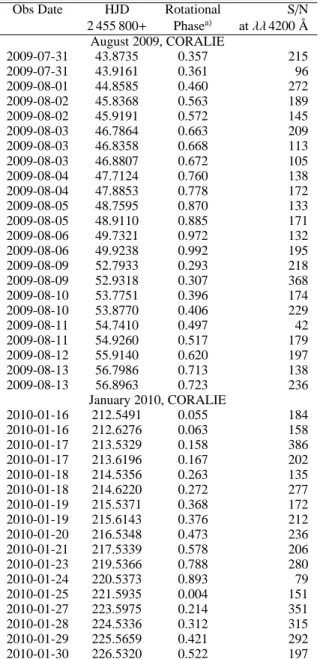
through-of 259 in the 2009 dataset and through-of 214 in the 2010 observations. More details on the observations, including the measured S/Ns, are given in the on-line Table 1 and the phases are also shown in Fig. 1.
For the data reduction the CORALIE on-line reduction pack-age with the usual steps of bias removal, flat-fielding, back-ground subtraction, and wavelength calibration using ThAr cal-ibration lamp is used. The final normalisation was done to the pipeline-merged spectrum using a cubic spline fit.
In the period analysis we also include five spectra taken in October 2005 and August 2006 with the FEROS ´echelle spec-trograph on the 2.2m telescope at the ESO La Silla observatory. These spectra cover the range 3530–9220 Å with a nominal re-solving power of 48 000.
In addition, we also use the HARPSpol observations of HD11753, which are publicly available in the ESO archive. HARPSpol is a polarimeter (Snik et al. 2011) feeding the HARPS spectrometer (Mayor et al. 2003) at the ESO 3.6m tele-scope in La Silla. More information on the observations them-selves can be obtained in Makaganiuk et al. (2012), and on the data reduction in Hubrig et al. (2012).
3. Orbital analysis
HD 11753 has been known to be radial velocity variable since the first spectrographic observations taken one century ago by Moore (1911) and then by Campbell & Moore (1928). Its vari-ability was confirmed by Dworetsky et al. (1982), who estimated the amplitude to be at least 12–15 km/s, but they were unable to determine the period. Combining these observations with new measurements, Leone & Catanzaro (1999) calculated a spectro-scopic orbit with a period of 41.49 days and a semi-amplitude of 9 km/s.
The long series of high-quality observations taken in the last few years are not consistent with the published orbit. We therefore carried out a general analysis of all the available ob-servations and found that the orbit in fact has a period of 1126 days. Radial velocities for the 153 CORALIE spectra, five FEROS spectra, and 13 HARPS spectra were measured by cross-correlations using a synthetic spectrum for Teff=11000 K and log g=4.0 as template. We also measured two mid-resolution (R=13000) spectra obtained with the REOSC spectrograph at the 2m telescope of the CASLEO (Complejo Astron ´omico El Leoncito, San Juan, Argentina).
Table 2, available at the CDS, lists our 173 radial ve-locity measurements and contains the following informa-tion: Heliocentric Julian Date, orbital phase, radial velocity measurement, error of the measurement, residual
observed-Fig. 2. Upper panel of the plot shows the radial velocity curve. Symbols are as follows: circles = CORALIE, (red) squares
= HARPS, (blue) filled triangles = FEROS, open triangles =
Leone & Catanzaro (1999), filled diamonds = Palomar plates of Dworetsky et al. (1982), crosses = SAAO plates of Dworetsky et al. (1982), and (green) pluses = Campbell & Moore (1928). Residuals observed-minus-calculated for our high-resolution measurements are shown in the lower panel.
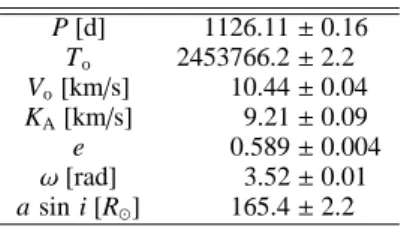
Table 3. Orbital parameters of HD 11753.
P [d] 1126.11 ± 0.16 To 2453766.2 ± 2.2 Vo[km/s] 10.44 ± 0.04 KA[km/s] 9.21 ± 0.09 e 0.589 ± 0.004 ω[rad] 3.52 ± 0.01 a sin i [R⊙] 165.4 ± 2.2
minus-calculated and the instrument information (H=HARPS, C=CORALIE, F=FEROS, R=REOSC). In addition we included three datasets from the literature in our analysis: six measure-ments from Leone & Catanzaro (1999), nine high-resolution spectrographic observations taken by Dworetsky et al. (1982) with the coud´e spectrograph of the Palomar 5m telescope, and 11 observations of lower resolution taken by the same authors with the coud´e spectrograph of the 1.9m telescope at SAAO.
The Lomb-Scargle method (Press & Rybicki 1989) was ap-plied to identify the period and a Keplerian orbit was fitted by the least squares method, obtaining the parameters listed in Table 3. The radial velocity curve is shown in Fig. 2.
The orbital phase coverage of the new observations (FEROS, CORALIE, HARPS) has unfortunately been very poor. All of them were concentrated around the flat maximum, with the only exception one FEROS spectrum taken at φ=0.03. This fact hindered the identification of the period in recent works (e.g., Paper 1; Makaganiuk et al. 2012) in spite of the large number of available observations.
Fig. 3. Radial velocity residuals as a function of rotational phase. Symbols are as in Fig. 2.
All high-resolution observations fit the newly calculated orbit very well, including the nine Palomar spectra taken by Dworetsky et al. (1982) for which the root mean square (RMS) of residuals is 0.22 km/s. Residuals of CORALIE, FEROS, and HARPS measurements have an RMS of 84 m/s. Part of this dis-persion is due to the line profile variability of HD 11753. In fact, the residuals show a clear one-wave variation as a func-tion of the rotafunc-tional phase (see Fig. 3), even though in cross-correlations we used a spectrum corresponding to solar chemi-cal abundance as a template so that the main peculiar lines (e.g., those of Y ii) have not contributed to our radial velocity mea-surements. After subtracting a soft curve to the residuals, we ob-tained an RMS of about 60 m/s, which can be considered as an estimate of the error of our CORALIE+FEROS+HARPS mea-surements. On the other hand, the Dworetsky et al. SAAO obser-vations have RMS=1.4 km/s and Leone & Catanzaro measure-ments RMS=0.5 km/s.
The calculated orbit is quite wide and eccentric. The orbital semiaxis is probably around 700–750 R⊙, and the secondary star mass would be in the range 0.9–1.7 M⊙. The minimum values in these ranges were calculated from the radial velocity ampli-tude assuming that the primary star has a mass of about 2.8 M⊙ (estimated from Teff=10 600 K, log g=3.8). The minimum val-ues were derived from the spectral lines of the companion star not being visible in the spectrum, and so the mass-ratio is prob-ably below 0.6. Since the separation at periastron is of the order of 300 R⊙, no interaction is expected to take place between the companions, and the observed chemical asymmetries in the pri-mary star surface are not related to binarity.
4. Doppler imaging
4.1. Period determination
All available datasets were used to determine the rotation pe-riod of HD 11753 using equivalent width (EW) measurements of seven Y ii lines: λλ4309.62, 4374.94, 4398.02, 4682.32, 4900.13, 5084.73, and 5662.95 Å. Figure 4 shows the peri-odogram calculated using the Lomb-Scargle method (Scargle 1982). The long time span of the observations allows an accu-rate determination of the period; a least-square fit of the sum of the EW of the seven Y ii lines with a cosine function yields
P = 9.53077 ± 0.00011 days. However, owing to the long
obser-vational gap between the years 2000 and 2009, with only a few FEROS spectra in between, there are also other periods,
sepa-Fig. 4. Periodogram from the sum of the equivalent widths of seven Y ii lines (left panel) and zoom around the adopted period (right panel).
rated by steps of 0.0273 days, that are compatible with the ob-servations, as can be seen in the right-hand panel of Fig. 4.
In addition to the rotational modulation of the line profiles, secular spectral variability is detected. Specifically, the EW of all the Y ii lines analysed here is approximately 10-20% (4-6 mÅ) higher in the 2000 datasets than in the 2009-2010 datasets. The behaviour of the Y ii line intensity with phase is shown in Fig. 5, where a global correction of +0.48 mÅ has been applied to 2009-2010 datasets in order to be able to plot the EW curves superimposed on each other. To show the secular variation more clearly, we removed the effect of rotational modulation using a least-square fit and plot the residual in the lower panel of Fig. 5. Parameters of the least-squares fit are listed in Table 4. FEROS data are not included in this analysis because the number of dat-apoints is too small for reliable determining the shape of the EW curve. Even though the behaviour of all the Y ii lines is very sim-ilar, a small long term change in the amplitude of the variations can be seen. We note that this behaviour is not instrumental be-cause it is not present, for example, in Ti ii and Cr ii lines (see Section 5.1).
To have an independent estimate of the period uncertainty we also calculated the period individually from the seven Y ii lines used in the previous analysis by fitting cosine curves to the data. Curves for individual lines can be seen in Fig. 6, and the resulting parameters are plotted in Fig. 7.
No significant evidence of any migration of surface spots is detected from the times of maximum Y ii abundance. Naturally, since the rotational period has been determined from Y ii abun-dance variations, global shifts in the phase cannot be detected (constant movement of the features would be interpreted as a different period), but abrupt movements of spots would still be measurable.
In the following Doppler imaging analysis, the newly de-termined period of 9.53077 days for the phase calculation is used, but we adopt the same T as was used in Paper 1, namely 2 451 800.0 With these ephemeris the intensity of Y ii lines is not maximum at φ = 0.00 as shown in Figs. 5 and 6, but at the phase
φ =0.8283.
Fig. 5. Equivalent width of Y ii lines. The average of seven Y ii lines is plotted for different epochs: CORALIE 2000 (open cir-cles), FEROS 2005-2006 (filled circir-cles), CORALIE 2009 (trian-gles), HARPSpol 2010 (squares), and CORALIE 2010 (stars). Lower panel: Secular variation of the mean equivalent width af-ter removing the rotational modulation.
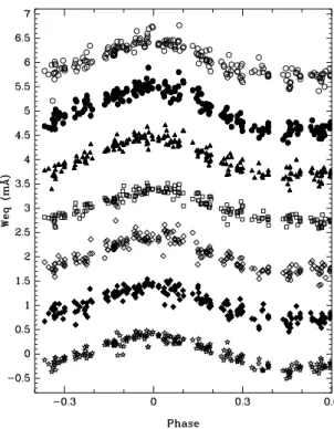
Fig. 6. Equivalent widths of seven Y ii lines as a function of the rotational phase. From top to bottom: λλ4309.62, 4374.94, 4398.02, 4682.32, 4900.13, 5084.73, and 5662.95 Å.
Table 4. Secular variation of Y ii curves. For the sum of the equivalent widths of seven Y ii lines, the mean value, amplitude, and time of maximum intensity is listed for five datasets.
Dataset mean JD mean EW EW semi-amplitude TYmax
mÅ mÅ Oct 2000 2 451 823.6 51.73±0.08 6.49 ±0.11 2 454 009.497±0.026 Dec 2000 2 451 887.7 52.18±0.16 5.99 ±0.22 2 454 009.445±0.051 Aug 2009 2 455 050.0 47.41±0.14 5.29 ±0.17 2 454 009.552±0.053 HARPS 2 455 207.3 47.14±0.05 5.59 ±0.05 2 454 009.491±0.014 Jan 2010 2 455 218.2 46.46±0.08 5.42 ±0.13 2 454 009.461±0.033
Fig. 7. Amplitude and period of the variations of seven Y ii lines.
4.2. Selection of spectral lines
In Paper 1 only one spectral line per element was used due to the possible radial stratification of the elements in the atmo-spheres of HgMn stars (e.g., Savanov & Hubrig 2003; Thiam et al. 2010). Makaganiuk et al. (2012) have investigated possible stratification of Ti ii and Y ii in HD 11753 and find very marginal indication of stratification in Y ii. For the current work, the line selection was based on the line identifications in a slowly rotat-ing HgMn star HD 175640 by Castelli & Hubrig (2004). Only non-blended lines that are detected in HD 11753 at a reasonable level are chosen for the analysis. For Sr ii only one non-blended line is available, namely Sr ii 4305.443 Å. The log g f values are mainly obtained either from VALD (e.g., Piskunov et al. 1995; Kupka et al. 1999) or from Makaganiuk et al. (2012). In the case of Y ii 5662.929 Å a slight adjustment to the log g f value was necessary to be able to fit all the Y ii lines simultaneously (value used here is 0.450, instead of 0.160 given in VALD and 0.384 used by Makaganiuk et al. 2012). The spectral lines used in this study and their parameters are given in Table 5.
4.3. Surface distribution of chemical elements in 2000-2010
We have obtained Doppler images of HD 11753 from CORALIE spectra for four different epochs. In Doppler imaging (see e.g., Vogt et al. 1987; Piskunov et al. 1990), spectroscopic observa-tions at different rotational phases are used to measure the rota-tionally modulated distortions in the line profiles. In HD 11753 these distortions are produced by the inhomogeneous distribu-tion of element abundance. Surface maps are constructed by combining all the observations from different phases and com-paring them with synthetic model line profiles. For the inversion we used the INVERS7PD code originally written by Piskunov (see, e.g., Piskunov 1991) and modified by Hackman et al. (2001). This code is based on Tikhonov regularisation. The local line profiles were calculated using the same methods and codes
Table 5. Spectral line parameters used in this study. The ion, cen-tral wavelength, excitation energy, log gf value, and the source of log gf are given. In the source M2012 means Makaganiuk et al. (2012)
Ion Wavelength [Å] Excit [eV] log gf source Y ii 4398.013 0.130 -1.000 VALD Y ii 4900.120 1.033 -0.090 VALD Y ii 5200.405 0.992 -0.570 VALD Y ii 5662.929 1.944 0.450 this work Sr ii 4305.443 3.040 -0.485 M2012 Ti ii 4163.644 2.590 -0.130 VALD Ti ii 4399.765 1.237 -1.190 VALD Ti ii 4417.714 1.165 -1.190 VALD Ti ii 4563.757 1.221 -0.690 VALD Cr ii 4145.781 5.319 -1.214 M2012 Cr ii 4275.567 3.858 -1.730 VALD Cr ii 4554.988 4.071 -1.438 M2012 Cr ii 4565.739 4.071 -1.980 VALD
as in Paper 1, except for the line selection and line parameters, which were both discussed in detail in the previous section. The CORALIE data obtained in 2000 have already been used for Doppler imaging of Y ii, Sr ii, and Ti ii lines in Paper 1, but then using the period determination based on 2000 data alone, and using one spectral line per element. Here, the new period deter-mination is adopted and, in most cases, four spectral lines have been used simultaneously in the inversion to obtain the map of that element. In addition, the regularisation parameter used in the inversion was changed to account for the weaker variability of Ti ii and Cr ii lines and to make the maps fully compatible with the maps of Makaganiuk et al. (2012). The August 2009 and January 2010 maps are previously unpublished, but some pre-liminary results have been presented in Korhonen et al. (2011).
As in Paper 1 we use vsin i=13.5 km/s for the inversions, ex-cept in the case of Sr ii where 12.5 km/s provides a much bet-ter fit. We run tests using the high-resolution HARPSpol ob-servations, and the results clearly show that the best fit to the Y ii, Ti ii, and Cr ii in the inversion process is obtained using vsini 13.5 km/s, whereas Sr ii requires smaller vsini. Similar difference in determined rotational velocity has been seen be-fore in HgMn stars, at least for Hg ii in HD 158704 (Hubrig et al. 1999. Makaganiuk et al. (2012) determine an inclination
i = 65.7◦±7.1◦ for HD 11753. We adopt here the inclination of 53◦that was used in Paper 1. This lower inclination gives us a
better fit than the higher value used by Makaganiuk et al. (2012). The Y ii distributions for the four datasets are shown in Fig. 8. The maps for all the four epochs (October 2000, December 2000, August 2009, and January 2010) show a high-abundance spot at the phases 0.75–1.0 extending from the equa-torial region all the way to the visible pole. Similarly in all the maps there is a lower abundance region around phases 0.2–0.4.
Fig. 8. Doppler maps of HD 11753 obtained from CORALIE data simultaneously from Y ii 4398.013 Å, 4900.120 Å, 5200.405 Å, and 5662.929 Å lines. Epochs of the maps are from top to bottom: October 2000, December 2000, August 2009, and January 2010. The surface distribution is shown for four differ-ent phases 0.25 apart. The maps from the year 2000 have already been published in Paper 1, but here they are shown using four Y ii lines simultaneously, using a refined regularisation parame-ter, and the newly determined period. The abundance scale for different epochs is the same.
Fig. 9. Same as in Fig. 8, but now for Sr ii line 4305.443 Å.
Fig. 10. Same as in Fig. 8, but now for Ti ii lines 4163.644 Å, 4399.765 Å, 4417.714 Å, and 4563.757 Å used simultaneously.
Fig. 11. Same as in Fig. 8, but now for Cr ii lines 4145.781 Å, 4275.567 Å, 4554.988 Å, and 4565.739 Å used simultaneously.
Since the rotation period was determined using EW of Y ii lines its abundance pattern is not expected to show any global longi-tude drift.
The Sr ii distribution is recovered using only the line at 4305.443 Å, because no other unblended Sr ii lines were avail-able for the analysis. The results for the four epochs are shown in
Fig. 9. All the maps show a very similar spot configuration with a strong high-abundance spot around the phases 0.75 to 1.0, and the rest of the stellar surface having a relatively low Sr ii abun-dance. The exact extent and configuration of the high-abundance regions change from epoch to epoch.
Figure 10 shows the Ti ii distributions for the four epochs. The spot distribution shows a main high-abundance spot around the phases 0.75–1.00, and patches of high and lower abundance elsewhere on the stellar surface. The lowest abundance is con-centrated around the phases 0.00 to 0.30.
In Fig. 11 the Cr ii distribution is shown for the four epochs. Again the highest abundances occur around the phases 0.75 to 1.00. The polar regions, on the other hand, always have low abundance, and the equatorial region is dominated by a high-abundance spot ring.
The observed spectral line profiles and the model fits to them are shown in the on-line Figs. 12–15 for Y ii and Figs. 16–19 for Cr ii. These two elements were chosen because examples as they show the strongest and weakest variability.
On the whole, at all epochs the main elemental spots retain quite stably their positions on the stellar surface the almost ten-year period our observations cover. The exact shape of the spots changes, though. Also, in all the maps, for different epochs and elements, all the abundances are higher than the solar abundance of that element.
In Hubrig et al. (2012) detailed analysis of the magnetic field in HD 11753 is carried out using HARPSpol data of January 2010. Their results show that there seems to be a correlation between the elemental spots and magnetic fields and their po-larities. Y ii and Ti ii lines reveal a weak negative magnetic field at the rotational phase 0.2 with 3σ significance. On the other hand, Cr ii and Fe ii show a weak positive magnetic field at phase 0.78, again with 3σ significance. These phases are ex-actly where our maps from January 2010 show the prominent el-emental spots, with the main high abundance spot around phase 0.75 and the main lower abundance spot at phases 0.2 to 0.4. Hubrig et al. (2012) find similar correlation between magnetic field polarity and low or high abundance spots also in other HgMn stars. Additional magnetic field measurements of these targets are needed to confirm these findings.
4.4. Comparison to the published maps
To test the reliability of our methods and codes, we also obtained elemental maps from the HARPSpol dataset, which was used by Makaganiuk et al. (2012) for obtaining elemental maps for Y ii, Sr ii, Ti ii, and Cr ii. We compared our results to their pub-lished maps. The core of the code used by Makaganiuk et al., INVERS10, is the same as in the code used here. Both codes have gone through several developments since the common ver-sion, INVERS7. The main differences are in the minimisation and coordinate system, where INVERS10 uses an equal sur-face area grid and INVERS7PD uses a cartesian coordinate sys-tem. Also the local line profiles are calculated differently in the two works. Here, the free available SPECTRUM code (Gray & Corbally 1994) has been used.
For this comparison we used the lines and line parameters given in Table 5 and the inclination of 53◦, as is also used for
our CORALIE data. On the other hand, the ephemeris used by Makaganiuk et al. (2012) is different from ours, so for an eas-ier comparison we have used their ephemeris for the HARPSpol data presented in Fig. 20. The results are virtually identical with the earlier published ones. The only slight difference is in the Cr ii map, where the low abundance spot at the phase 0.5 is more
Fig. 20. Doppler maps of HD 11753 from January 2010 data ob-tained with HARPSpol. The maps are from top to bottom: Y ii, Sr ii, Ti ii and Cr ii. These same data have been used for Doppler imaging by Makaganiuk et al. (2012). Here, same lines and in-clination angle as for the CORALIE datasets have been used, but now the ephemeris is from Makaganiuk et al. (2012) to enable an easy comparison. The results are presented from the same phases as used by Makaganiuk et al. (2012), and are virtually identical to theirs.
pronounced in our map than in the one by Makaganiuk et al. (2012).
4.5. Comparison of the maps obtained from 2010 January CORALIE and HARPSpol data
A target with a low v sin i, like HD 11753, would ideally re-quire observations from an instrument with a very high resolv-ing power, like HARPSpol. CORALIE’s resolvresolv-ing power of
∼55,000 is relatively low, and therefore it is important to estab-lish what effect that has on the resulting maps.
The 2010 January CORALIE dataset and 2010 January HARPSpol data were basically obtained immediately after each other with the HARPSpol dataset spanning the first half of January and the CORALIE dataset the second half. Here we compare maps obtained from these two datasets, which should not really show differences in spot configurations, but are ob-tained with different instruments. HARPSpol S/N and resolution are superior to the CORALIE one, therefore providing a crucial test of the usability of CORALIE observations for the Doppler imaging of HD 11753.
Figure 21 shows the result for the 2010 January CORALIE and HARPSpol data. The model fits the HARPSpol observations of Y ii and Cr ii are given in the on-line Figs. 22 & 23, respec-tively. On the whole the spot configurations in the maps are vir-tually identical for the strongly variable lines of Y ii and Sr ii. Also, Ti ii results are very similar with small differences in the lower abundance spot at phases 0.2 to 0.4. The biggest differ-ences are seen in the least variable element Cr ii, where the
equa-Fig. 21. Comparison between CORALIE (left) and HARPSpol (right) January 2010 maps. The ephemeris is the same as used for CORALIE data in this paper.
torial high abundance spot around the phase 0.0 is not seen in the CORALIE data. Otherwise even the Cr ii maps are very similar. The differences in the equatorial spot belt around the phases 0.6 to 0.7 can be explained by the phase gap in the CORALIE data spanning phases 0.58 to 0.79.
From this comparison it is clear that CORALIE data can be used for Doppler imaging of a relatively slowly rotating star, like HD 11753.
4.6. Impact of phase gaps in the data
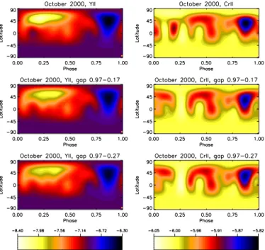
The dataset from October 2000 has an excellent phase coverage with the largest phase gap around 0.1 in phase. Unfortunately, there are larger gaps for the other datasets: 0.16 in phase for 2010 January HARPSpol data (0.36–0.52), 0.20 in phase for December 2000 (phases 0.19–0.39), 0.21 for January 2010 (phases 0.58-0.79), and 0.30 for August 2009 (phases 0.00-0.30). To study the effect of these phase gaps in the maps a test was done using the October 2000 dataset that removed all the observations between phases 0.00 and 0.20/0.30 to simulate the size and location of the largest phase gap (August 2009 data). The resulting maps for Y ii and Cr ii are shown in Fig. 24. The figure shows the original map and maps with the 0.2 and 0.3 phase gaps. Tests were carried out using Y ii and Cr ii because these are the elements with the largest and smallest variability, respectively.
Removing the phases 0.00–0.30 affects the exact determina-tion of the shape of the spots at this phase range. Still, on the whole the Y ii map is very similar to the original map without the phase gap, the location of the spots has not changed, but the high latitude low abundance feature is less prominent. In the case of Cr ii, which shows much weaker variability, the recovery of spots in the phase gap is seriously affected. The high abun-dance spot around the phase 0.18 is basically not recovered, and the exact shape of the high abundance spot at the phase 0.05 is also significantly affected.
Fig. 24. Phase gap tests using 2000 October CORALIE data for the Y ii (left) and Cr ii (right) lines. The top figure is the original map, middle one has phases 0.97–0.17, removed and the bottom one phases 0.97–0.27 removed.
From this it can be concluded that, especially in the case of lines with weak variability, Ti ii and Cr ii, one has to be careful when interpreting spot features when the phase coverage is not optimal. The recovery of the surface features in the strongly vari-able lines is not as affected by the phase gaps. Naturally also the exact spot configuration has an effect on the recovery, because large spots are less affected by phase gaps.
5. Discussion
5.1. Long-term abundance evolution
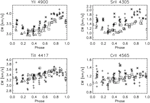
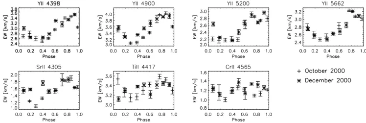
For investigating long-term changes in the elemental spots in HD 11753 we have also measured equivalent widths from all the CORALIE datasets for the lines we have used in the inversions. Examples of the results for each element are shown in Fig 25.
As already pointed out in Section 4.1 the equivalent width in Y ii decreases with time. This is seen in all the lines used in the inversions. In addition the same effect is clearly seen for Sr ii. This effect is not just present in the 4305.443 Å line used here, but for example Sr ii 4215.519 Å line shows it, too. The dimin-ishing abundance is also clearly seen in the Y ii and Sr ii maps in Figs. 8 & 9. On the other hand, no significant long-term change is seen in the Ti ii and Cr ii equivalent widths.
We want to emphasise that the maps of chemical elements obtained here and the conclusions about the evolution of their surface distribution, are not affected in any significant manner by the possible ambiguity in the rotational period (see Fig.4), since the maps are calculated with observations from one relatively short run. In the same manner, the differential rotation discussion in Section 5.3 would remain unchanged, since it is based on a differential analysis of the spot patterns.
Fig. 25. Equivalent width measurements from the CORALIE data at different epochs. The results for four different elements are shown for October 2000 (plus), December 2000 (asterisk), August 2009 (square), and January 2010 (triangle). The ordinates have very different scales.
5.2. Fast chemical spot evolution
In Paper 1 fast chemical spot evolution within the 65 days be-tween the October 2000 and December 2000 maps was reported. Here we look into this in more detail.
To investigate how many random changes one would ex-pect in the maps with the current data quality, the October 2000 dataset was divided into two subsets. The division was done by taking every other phase for part 1 and the other for part 2, without any overlap in the data. Because our complete dataset for October 2000 has excellent phase coverage, and also many observations from similar phases (76 phases), this dataset was chosen for the test. The effect of the division of 2000 October data into two subsets is effectively only lower S/N per phase in the inversion, but with similar phase coverage as in the original dataset.
The maps for all the elements from the original 2000 October dataset, part 1, part 2, and original 2000 December datasets are shown in Fig 26. As can be seen, the original October 2000 map and the maps from parts 1 and 2 are virtually identical for all the elements, except for Cr ii where the part 1 map is missing the equatorial extension of the high abundance spot around the phase 0.3. Otherwise the parts 1 and 2 maps of Cr ii are also very similar to the original one.
The abundance scales for all the elements are slightly differ-ent for maps obtained from part 1 and part 2. This implies that the abundance scale in general in the maps is on average accu-rate to ∼4%. In most cases the variation in the maximum and minimum abundance in the part 1 and part 2 maps is 0.2–5.6% of the full abundance range in the particular map. There are two notable differences, though, the maximum Cr ii abundances in the two maps show a difference of 7.4% of the full abundance range, and minimum Y ii abundances show a difference of 12%. The December 2000 maps are more different from the October 2000 maps, than the maps from the divided datasets are from the original October 2000 maps. This is true for all the el-ements, and implies that an evolution of the chemical spots has
occurred during the 65 days between the 2000 October and 2000 December datasets.
In Y ii both the high abundance spot around the phase 0.75 and the lower abundance spot around the phase 0.25 get less prominent and at the same time more extended with time. The equatorial extension of the low abundance spot at the phase of 0.25 seen in the December 2000 map could be due to missing observations at phases 0.19 to 0.39, but it would not explain the extension of the low-abundance spot towards later phases, and the wider high abundance spot at the higher latitudes.
For Sr ii the over-all abundance at phases 0.2 to 0.5 is higher in December 2000 than it is in October 2000. In addition the high abundance spot at phase 0.5 has become more prominent with time. One has to remember, though, that the Sr ii maps are obtained from only one spectral line.
In the case of Ti ii the low-abundance feature at the phase 0.5 does not have as low an abundance in December 2000 as it has in October 2000, and the low abundance feature around the phase 0.7 is more prominent in December 2000. Cr ii, on the other hand, exhibits an extended low-abundance high-latitude feature around the phase 0.5 in the December 2000 map. This feature is not present in the October 2000 Cr ii map. One should keep in mind that the spectral variability is relatively weak in Ti ii and Cr ii.
We also investigate whether the effects can be seen in the equivalent width measurements. This is more demanding, be-cause the behaviour of equivalent width does not directly reflect the element distribution, but is an integral value and can appear almost constant even if the distribution of the element is slightly changing on the surface. Figure 27 shows the equivalent width measurements for the 2000 October and 2000 December datasets in all the Y ii and Sr ii lines used in the inversions, and also exam-ples for Ti ii and Cr ii lines. The 2000 October measurements are from the first full stellar rotation of that dataset. Each datapoint is the mean of all the observations obtained within one night, and the standard deviation of the measurements provides the
er-Fig. 26. Investigating the fast temporal evolution of the elemental spots. The figures show original October 2000 map, October 2000 map from half of the data, October 2000 map from the other half of the data and the original December 2000 for all the elements. The elements are from left to right: Y ii, Sr ii, Ti ii, and Cr ii.
Fig. 27. Equivalent width measurements from October and December 2000 datasets for all the Y ii and Sr ii lines used in inversion and examples of Ti ii and Cr ii measurements. The values are from the first stellar rotation in October 2000 (plus) and last rotation in December 2000 (asterisk). The value is the mean of the observations obtained within one night. The error is the standard deviation of the measurements. The ordinates have different scales.
ror. The 2000 December measurements are treated similarly, but now the last full stellar rotation is used.
In general the equivalent width measurements for October 2000 and December 2000 are very similar, but there are some differences. The equivalent widths for Y ii 4900.120 Å in December 2000 are clearly larger in phases 0.4 to 0.6 than they are in October 2000 at the same phases. Similar trends are also seen in Y ii 4398.013 Å and 5200.405 Å, but they are less
promi-nent. Equivalent widths for Sr ii 4305.443 Å, on the other hand, show very clear differences at phases 0.2 to 0.5, with higher values in December 2000. This behaviour is also seen in Sr ii 4215.519 Å, which was checked for consistency, and is in line with what is seen in the Sr ii maps for the year 2000 (Fig. 26). Both Ti ii 4417.714 Å and Cr ii 4565.739 Å lines show much less variability than the lines of the other elements, but the ten-dency for the measurements at phases 0.4–0.6 to have higher
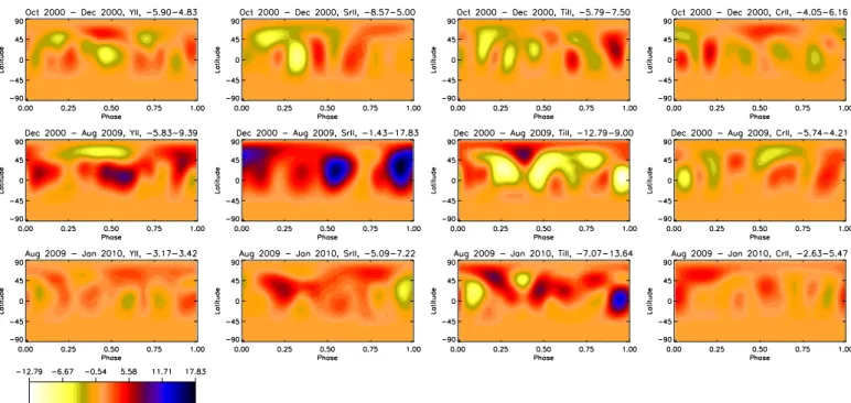
Fig. 28. The significance of the changes between two consecutive epochs. The elements are from left to right: Y ii, Sr ii, Ti ii, and Cr ii. The figure gives standard deviation of the change for the following epochs: October 2000 December 2000, December 2000 -August 2009, and -August 2009 - January 2010, from top to bottom. The original difference maps have been divided by the standard deviation of the difference for the October 2000 part 1 – part2 map, to present the significance of the changes. All the significance maps have the same scale, and the scale for each map is given in the title of the individual plot. Colour-coding is such that the dark colour indicates higher abundance in the first map from which the second map is subtracted; similarly, bright colour indicates lower abundance in the first map.
Table 6. Standard deviation of the difference maps.
Difference map Y ii Sr ii Ti ii Cr ii Oct 2000: part1 – part2 0.077 0.023 0.014 0.019
Oct 2000 – Dec 2000 0.132 0.044 0.029 0.031 Dec 2000 – Aug 2009 0.215 0.091 0.049 0.034 Aug 2009 – Jan 2010 0.087 0.045 0.042 0.026
values in December 2000 than in October 2000 is still seen in Ti ii 4417.714 Å.
Finally, the significance of the detected changes was evalu-ated. First, difference maps between consecutive epochs for all the elements were calculated, e.g., subtracting the abundances of December 2000 map from the abundances of October 2000 map for Y ii. The amount of changes seen in the difference maps of the two October 2000 submaps (parts 1 and 2 from Fig. 26) is taken to be the detection limit of the variation. In the signifi-cance maps presented in Fig. 28, the difference maps are divided by the standard deviation of the difference part1 - part2 of that element to show the standard deviation of the change. The plot gives October 2000 - December 2000, December 2000 - August 2009, and August 2009 - January 2010, from top to bottom, and Y ii, Sr ii, Ti ii, and Cr ii from left to right.
In addition, the standard deviation of each difference map is calculated and results given in Table 6. The changes seen in the earlier analysis of the maps and equivalent width measurements are confirmed by the difference maps. In most cases the standard deviation of the difference map is twice, or more, than of the deviation part1 - part2 for that element.
Subtracting the December 2000 map from the October 2000 one in Y ii still indicates that the high-latitude, lower abundance spot at phases 0.0–0.4 extends more towards phase 0.5 in the
December 2000 map, and that at the same time the lower abun-dance spot has become less prominent. The biggest differences in the Y ii abundance are seen in the equatorial region around phase 0.5. This is caused by a high abundance spot at this loca-tion in the December 2000 map, that is not present in the October 2000 map, nor in the August 2009 map. Also, the virtual disap-pearance of the lower abundance spot at high latitudes around phases 0.2 to 0.4 between December 2000 and August 2009 is also confirmed. This change cannot be completely explained by the missing phases 0.0 to 0.3 in the August 2009 map, because the difference is clearly seen also at phases 0.3 to 0.6. In addi-tion, it is clear that in many regions the abundance in the August 2009 map is lower than in the December 2000 map. On the other hand, there are basically no significant changes between August 2009 and January 2010 in Y ii.
In the Sr ii difference maps, the changes between October 2000 and December 2000 are confirmed, and the higher abun-dance in December 2000 around the phase 0.3 is seen well. The overall change in the abundance between December 2000 and August 2009 is clear, and especially the high abundance spot around the phase 0.75 becomes less extended. Again the changes between August 2009 and January 2010 are small, with the higher abundance around phases 0.1 to 0.3 in the August 2009 map being the main difference. One has to remember, though, that in August 2009 map the observations are missing from phases 0.0 to 0.3, and the difference in the abundances could be caused by the phase gap.
In the Ti ii difference maps the largest changes are seen in the abundance of the main low abundance spot around the phase 0.9. Changes in the exact spot configurations in other locations are also seen, and it seems that the August 2009 map is different from the others. This is verified by subtracting January 2010 map
diamonds, and Cr ii with (black) circles. The relative rotation pe-riods at different latitudes obtained from different elements are remarkably similar. The average errorbar of the measurements is given in the upper left corner.
from the December 2000 map; the differences are clearly smaller than between December 2000 and August 2009. Cr ii difference maps imply very small changes in the exact spot configurations at a wide range of locations.
5.3. Investigating possible surface differential rotation
We applied the spot-centre tracking technique for the detection of stellar velocity fields to the time series of Doppler maps. The method will be tested and explained in detail in Flores Soriano et al. (in preparation). We describe here the basics of the process and the steps taken.
To reduce the effects of spot evolution and artefacts, only spots that can be unambiguously identified at the five different epochs (maps from CORALIE data and also from HARPSpol data presented in Section 4.4) are used. This limits our analy-sis to the most prominent overabundance features. The border of the spot is chosen as the abundance that maximises its size with-out been affected by neighbour structures or potential artefacts. In this case, we chose −5.89 for Cr, −7.1 for Sr, −6.44 for Ti, and −6.8 for Y. When spurious spots are also isolated, they are removed and not considered in the analysis. Since all spots are at a similar latitude, it is not possible to unambiguously detect a latitudinal dependence of the rotation period by measuring the motion of the spots as a whole. Nevertheless, their large extent means it remains viable to calculate it by measuring the rota-tion period in different latitude bands. For doing this the maps were divided into equal-latitude strips, each one with a width of 4.5◦, equal to the pixel size in the maps. For the region of the
spot enclosed in each band, the coordinates of its centre are cal-culated as an “abundance centre” (in analogy to the centre of mass) where areas with an abundance lower than the selected limit make no contribution. Latitudinal rotation rates are calcu-lated by fitting the evolution of the longitude as a function of time to a line.
According to our results, the rotation period is minimum near the equator and gradually increases until latitude 65◦, where it
reaches a value that is ∼115 seconds higher. As can be seen in Fig. 29, the rotation periods relative to the mean rotation period obtained from all the maps (Y ii, Sr ii, Ti ii, and Cr ii) are in ex-cellent agreement with each other. The relative rotation periods
from different elements at the same latitude are averaged, and the resulting profile fitted with the usual differential rotation law:
Ω(θ) = Ωeq − ∆Ω sin2θ
where θ is the latitude, Ωeq the equatorial rotation rate, and
∆Ω = Ωeq − Ωpole. The results are also shown in Fig. 30. We
obtain a surface shear of ∆Ω = 0.098 ± 0.023 mrad/day, equiv-alent to a lap time (time the equator needs to lap the pole) of approximately 175 years. The derived equatorial rotation period is 9.53123 ± 0.00012 days, i.e., 40 seconds longer than found with equivalent widths (see Section 4.1). Evidence of differen-tial rotation in late B-type star has been found before only in one target, the B9 star HD 174648 (Degroote et al. 2011).
6. Conclusions
From the investigation of high-resolution spectra of HD 11753 in four different epochs, the following conclusions can be drawn: – We determined the binary orbit of HD 11753. The radial ve-locity measurements can be explained by a wide and eccen-tric orbit with orbital period of 1126 days.
– We fine-tuned the rotation period determination of HD 11753 using data spanning almost ten years.
– HD 11753 clearly exhibits inhomogeneous distribution of Y ii, Sr ii, Ti ii, and Cr ii, with the main high abundance fea-ture occurring at the same phase in all the elements. – The most prominent features in the maps remain at similar
location for the duration of the observations (10 years), but the exact shapes and abundances change.
– Both fast and secular evolution is seen in the spot configura-tions, with the spot configurations changing even on monthly time scales, and the mean abundance of Y ii and Sr ii chang-ing on yearly time scales.
– Some indications of very weak surface differential rotation is seen using the spot-centre tracking technique.
Acknowledgements. HK acknowledges the support from the European Commission under the Marie Curie IEF Programme in FP7. SH and JFG ac-knowledge the support by the Deutsche Forschungsgemeinschaft (Hu532/17-1). The authors wish to thank Gaspare Lo Curto from ESO/Garching for his help with the ESO HARPS pipeline when reducing the HARPSpol data obtained from the archive. The authors also thank the referee, Dr. John Landstreet, for his comments that helped to improve this paper.
References
Adelman, S.J., Gulliver, A.F., Kochukhov, O.P., & Ryabchikova, T.A. 2002, ApJ, 575, 449
Bagnulo, S., Landstreet, J.D., Fossati, L., & Kochukhov, O. 2012, A&A, 538, A129
Briquet, M., Korhonen, H., Gonz´alez, J.F., Hubrig, S., & Hackman, T. 2010, A&A, 511, 71
Campbell, W. W., & Moore, J. H. 1928, Pub. Lick Obs., 16, 22 Castelli, F., & Hubrig, S. 2004, A&A, 425, 263
Degroote, P., Acke, B., Samadi, R., et al. 2011, A&A 536, A82 Dolk, L., Wahlgren, G.M., & Hubrig, S. 2003, A&A 402, 299
Dworetsky, M. M., Stickland, D., F., Preston, G. W., & Vaughan, A. H. 1982, Obs 102, 145
Folsom, C.P., Kochukhov, O., Wade, G.A., Silvester, J., & Bagnulo, S. 2010, MNRAS, 407, 2383
Gray, R.O.,& Corbally, C.J. 1994, AJ, 107, 742
Hackman, T., Jetsu, L., & Tuominen, I. 2001, A&A, 374, 171 Hubrig, S., Castelli, F., & Mathys, G. 1999, A&A, 341, 190
Hubrig, S., Gonz´alez, J.F., Savanov, I., et al. 2006a, MNRAS, 371, 1953 Hubrig, S., North, P., Sch¨oller, M., & Mathys, G. 2006b, AN, 327, 289 Hubrig, S., Savanov, I., Ilyin, I., et al. 2010, MNRAS, 408, L61 Hubrig,S., Gonz´alez, J.F., Ilyin, I., et al. 2012, A&A, 547, A90
Kochukhov, O., Adelman, S.J., Gulliver, A.F.,& Piskunov, N. 2007, Nature Physics, 3, 526
Korhonen, H., Hubrig, S., Briquet, M., Gonz´alez, F., & Savanov, I. 2011, IAUS 273, p.116
Kupka, F., Piskunov, N.E., Ryabchikova, T.A., Stempels, H.C., & Weiss, W.W. 1999, A&AS, 138, 119
Leone, F., Catanzaro, G. 1999, A&A, 343, 273
Makaganiuk, V., Kochukhov, O., Piskunov, N., et al. 2011, A&A, 525, 97 Makaganiuk, V., Kochukhov, O., Piskunov, N., et al. 2012, A&A, 539, A142 Mathys, G. 1991, A&AS, 89, 121
Mathys, G. 1995a, A&A, 293, 733 Mathys, G. 1995b, A&A, 293, 746
Mayor, M., Pepe, F., Queloz, D., et al. 2003, The ESO Messenger, 114, 20 Moore, J. H. 1911, Lick. Obs. Bull., 6, 150
Piskunov, N.E. 1991, in The Sun and Cool Stars, Activity, Magnetism, Dynamos, ed. I. Tuominen, D. Moss, & G. Rdiger (Heidelberg: Springer-Verlag), Lecture Notes in Physics, 380, IAU Colloq., 130, 309
Piskunov, N.E., Tuominen, I.,& Vilhu, O. 1990, A&A, 230, 363
Piskunov, N.E., Kupka, F., Ryabchikova, T.A., Weiss, W.W., & Jeffery C.S. 1995, A&AS, 112, 525
Press, W. H., Rybicki, G. B. 1989, ApJ, 338, 277 Renson, P.,& Manfroid, J. 2009, A&A 498, 961 Savanov, I., & Hubrig, S. 2003, A&A,410, 299
Savanov, I.S., Hubrig, S., Gonz´alez, J.F., & Sch¨oller, M. 2009, IAUS 259, p.401 Scargle, J.D. 1982, ApJ, 263, 835
S´egransan, D., Udry, S., Mayor, M., et al. 2010, A&A, 511, A45 Snik, F., Kochukhov, O., Piskunov, N., et al. 2011, ASPC, 437, 237S Thiam, M., LeBlanc, F., Khalack, V., & Wade, G.A. 2010, MNRAS, 405, 1384 Vogt, S.S., Penrod, G.D.,& Hatzes, A.P. 1987, ApJ, 321, 496
2009-08-05 48.9110 0.885 171 2009-08-06 49.7321 0.972 132 2009-08-06 49.9238 0.992 195 2009-08-09 52.7933 0.293 218 2009-08-09 52.9318 0.307 368 2009-08-10 53.7751 0.396 174 2009-08-10 53.8770 0.406 229 2009-08-11 54.7410 0.497 42 2009-08-11 54.9260 0.517 179 2009-08-12 55.9140 0.620 197 2009-08-13 56.7986 0.713 138 2009-08-13 56.8963 0.723 236 January 2010, CORALIE 2010-01-16 212.5491 0.055 184 2010-01-16 212.6276 0.063 158 2010-01-17 213.5329 0.158 386 2010-01-17 213.6196 0.167 202 2010-01-18 214.5356 0.263 135 2010-01-18 214.6220 0.272 277 2010-01-19 215.5371 0.368 172 2010-01-19 215.6143 0.376 212 2010-01-20 216.5348 0.473 236 2010-01-21 217.5339 0.578 206 2010-01-23 219.5366 0.788 280 2010-01-24 220.5373 0.893 79 2010-01-25 221.5935 0.004 151 2010-01-27 223.5975 0.214 351 2010-01-28 224.5336 0.312 315 2010-01-29 225.5659 0.421 292 2010-01-30 226.5320 0.522 197
Notes. a) calculated using P=9.53077 and T=2 451 800.0
Fig. 12. October 2000 CORALIE observations (thin line) to-gether with the model fit (thick line) for Y ii lines used in Doppler imaging (map in Fig. 8).
Fig. 13. Same as on-line Fig. 12 except now for December 2000 CORALIE Y ii observations.
Fig. 14. Same as on-line Fig. 12 except now for August 2009 CORALIE Y ii observations.
Fig. 15. Same as on-line Fig. 12 except now for January 2010 CORALIE Y ii observations.
Fig. 16. Same as on-line Fig. 12 except now for October 2000 CORALIE Cr ii observations.
Fig. 17. Same as on-line Fig. 12 except now for December 2000 CORALIE Cr ii observations.
Fig. 18. Same as on-line Fig. 12 except now for August 2009 CORALIE Cr ii observations.
Fig. 19. Same as on-line Fig. 12 except now for January 2010 CORALIE Cr ii observations.
Fig. 22. Same as on-line Fig. 12 except now for January 2010 HARPSpol Y ii observations.
Fig. 23. Same as on-line Fig. 12 except now for January 2010 HARPSpol Cr ii observations.