8.1. Introduction
Control and state estimation of dynamical systems subject to impacts are rel-evant problems in several application areas, often related to the robotics field [BRO 99]. Impacts play a key role in several studies including hopping robots (see, e.g., [SCH 95]), walking robots (see, e.g., [MOR 09]) and juggling robots (see, e.g., [RON 06]). Several Lyapunov-based solutions to the stabilization and tracking problems of systems with impacts have been proposed in the past decade [BRO 04, LEI 08a, TOR 99], and several studies have been developed for the dual state-estimation problem [MEN 01c, MEN 01b, GAL 03]. Some of them address the problem via the larger class of complementarity Lagrangian systems (see [HEE 03] for a survey, and the overview in [MOR 10] which also generalizes and improves the results in [BOU 05, BRO 97]). Within this field, tracking in billiards is a relevant and representative example where much has been done using the model first proposed in [TOR 99]. See [GAL 08] and references therein. Several additional recent techniques addressing tracking control with impacts both from a theoretical and an experimental viewpoint are provided in the works [PAG 01, PAG 04, LEI 08b, MEN 01a, SEK 06] and references therein. See [MOR 10] for a more detailed overview.
One important obstruction to effective tracking and state observation laws for sys-tems with impacts is that when stabilizing the error dynamics (associated with track-ing or observation laws), classical continuous-time solutions that disregard the effects of the impacts may not work properly due to the undesired effects of impacts. We show in Section 8.2 that even a simple linear exponential tracking for a one dimen-sional system may produce an unstable error dynamics when applied to the impacting dynamics. An alternative example with a similar flavor and a formal analysis of insta-bility has been also given in [FOR 11a]. Motivated by this obstruction and the goal of
Chapter written by F. FORNI, A.R. TEEL and L. ZACCARIAN.
recovering linear error dynamics, in our recent work [FOR 11b, FOR 11c, FOR 11a], we formulated the tracking and observation problems for a mass moving in a pla-nar confined region as a hybrid stabilization problem for a suitable set. In particu-lar, by casting the tracking or observation problems within the hybrid framework of [GOE 06, GOE 12, GOE 09], asymptotic tracking or estimation is written as an expo-nential stabilization problem for a closed set (or attractor) A where certain relevant sub-states are equal. The core ideas of [FOR 11b, FOR 11c, FOR 11a] have been later extended in [FOR 12] to the case of a mass moving into an n dimensional half space. Similar ideas to those in [FOR 11b] were independently presented later as an appli-cation of the Lyapunov conditions in [BIE 12, BIE 13], with special emphasis on the one-dimensional case of a bouncing ball.
In this book chapter we illustrate the main ideas behind [FOR 11b, FOR 11c, FOR 11a, FOR 12] by emphasizing the fundamental intuition behind our approach, which allows to recover a classical (quasi-)linear control algorithm for tracking and state-estimation of point-masses evolving in an n-dimensional space in the presence of impacts. Given a controlled (or observer) system and a reference system with state vectors x and z respectively, we replace the usual feedback error e = x−z by a gener-alized error e = x − m(q, z). The logic variable q is typically updated at each impact and keeps track of the (finite set of) impact phenomena Q := {1, . . . , d}. The func-tion m(q, z) is an affine transformafunc-tion on z that ensures the non-increase of the error magnitude at impacts, as measured by a suitable quadratic error Lyapunov function. The introduction of the generalized error e is driven by the suggestive idea that the effect on an impact on a boundary can be virtually inverted by using the boundary as a mirror. In this sense, the transformation m(q, z) provides the control algorithm with a feedback measurement of a suitable mirrored reference motion “through” the mir-ror/boundary, with the goal of recovering the exponential decrease of the error along the trajectories of the (hybrid) closed-loop system.
In this chapter we illustrate the intuition above by addressing several examples where the loss of performance experienced with linear controllers is recovered by the introduction of the generalized error e = x − m(q, z). We start our discussion with a one-dimensional system in Section 8.2, whose dynamics resembles that of a bouncing ball even though the engineering motivation behind this example is somewhat more intuitive. We then discuss a slightly more complicated example of a Newton cra-dle, using a model taken from the literature [MEN 02] and showing that similar ideas apply here too. We then move on to a much more general system where a mass is constrained to evolve in an equilateral triangular subset of the position subspace. The construction of the mirrored references m(q, z) for this case becomes more involved and is illustrated graphically to preserve the intuitive style of the chapter. Finally, in Section 8.5 we address an apparently different estimation problem where there is no need to define mirrored references and the analysis then greatly simplifies.
Each one of the discussed examples contains a hybrid formulation of the impacting dynamics together with the proof of a key property about the behavior of the gener-alized error e = x − m(q, z) across impacts, which can be derived from the jump dynamics of the hybrid model. Then, a theorem states exponential convergence to zero of the generalized error and a proposition illustrates how one can draw suitable conclusions on the actual error x − z from properties of the generalized error (this is not necessary for the last example where no mirrors are used). All the theorems stating exponential convergence are proven using the results in [TEE 12] and to better highlight the strong commonalities among the proofs (despite the very different nature of all the examples), the proofs of these theorems are gathered together in Section 8.6, where a Lyapunov reformulation of [TEE 12, Theorem 2] is also given to facilitate the analysis.
Notation:For any given vector z ∈ "2n, z
idenotes the ith component of z, zp(positions) denotes the sub-vector given by z1, . . . , zn, and zv(velocities) denotes the sub-vector given by zn+1, . . . , z2n. Inis the identity matrix of dimension n. Given two matrices A and B, their Kronecker product is denoted by A ⊗ B.
8.2. Hammering a surface
The first example that we propose is a mechanical system with one degree of free-dom experiencing impacts comprising a hammer hitting on a surface. This exam-ple clearly illustrates the possible dangers of blindly using linear tracking controllers whenever impacts are experienced. Similar results have been presented for a bounc-ing ball in [FOR 11b, FOR 11a]. The hammer formulation of the same phenomenon perhaps has a better engineering motivation.
8.2.1. The reference hammer dynamics
Let us consider the reference dynamics Z of a hammer impacting on a surface, as shown in Figure 8.32. The angular position of the hammer with respect to the horizontal line is represented by the state variable zp, while its angular velocity is
denoted by zv. The hammer is driven towards the plane by the concurrent action of
a spring, which exerts the torque −kszp(where ks > 0 is the spring characteristic
constant) at the hinge, and of the gravity that, assuming for simplicity unit mass, generates the torque −g cos(zp) at the hinge. The dynamics of the system is given by
¨
zp=−kszp− g cos(zp) z∈ Cz :={(zp, zv)∈ #2: zp∈ [0, π]}, (8.250)
where the closed set Cz ⊂ #2is instrumental to restricting the position z1of the
hammer to the upper half plane of Figure 8.32. Indeed, solutions that would reach beyond those points are prematurely terminated by the fact that they cannot flow (nor jump).
zp
g
Figure 8.32: The reference hammer impacts on the horizontal plane. Using the aggregate state z := [ zp zv]T, a convenient formulation of the flow
dynamics (8.250) is given by ˙z = Az + Bαz(z) z∈ Cz (8.251a) where A := ! 0 1 0 0 " , B := ! 0 1 " , αz(z) :=−kszp− g cos(zp). (8.251b)
which highlights the structure of a double integrator driven by (possibly nonlinear) state dependent acceleration terms.
At impacts, the sign of the speed zv is inverted, while the position zp remains
constant. However, due to the convenient selection of the coordinate system where impacts occur only if zp = 0, we can write the impact (or jump) dynamics of the
hammer as: z+= ! zp −zv " = ! 0 −zv " =−z, z ∈ Dz:={(zp, zv)∈ #2: zp= 0, zv≤ 0}, (8.252) namely, similar to the well studied example of a bouncing ball (see, e.g., [GOE 09, Example 3]) the specific selection of the coordinate system simplifies the jump map.
The combination of the flow dynamics (8.251) and the jump dynamics (8.252) and the flow and jump sets Cz, Dzprovide a hybrid formulation of the reference hammer
dynamics, according to the notation proposed in [GOE 12, GOE 09]. For dealing with this example and the rest of the examples treated in this chapter we will use results from this specific framework for describing hybrid dynamical systems. We don’t recall here the essential definitions from [GOE 12, GOE 09]. The reader is referred to those works for an introduction of that framework or, alternatively, to the brief overview in [NE˜11, Section II].
8.2.2. Using dwell-time logic to avoid Zeno solutions
Both the flow set Czand the jump set Dzin the hybrid model (8.251), (8.252) are
solutions set of our hybrid system are guaranteed (see, e.g, [GOE 12, Chapter 6]). Due to this reason, some solutions may exhibit an infinite number of jumps (namely a Zeno behavior) when starting from the initial condition with z1= 0 and z2= 0. To avoid
this particular side effect of the adopted dynamical model, we embed in our dynamics a so-called average dwell time logic, as characterized in the appendix of [CAI 08] (see also [GOE 12, Example 2.15]) parametrized by a real ρ > 0 and an integer N ≥ 1 and satisfying the flow and jump equations:
˙σ ∈ [0, ρ], σ∈ [0, N]
σ+ = σ− 1, σ∈ [1, N] . (8.253)
As formally proven in [CAI 08, Proposition 1.1], embedding the extra state σ in the hybrid description and intersecting the sets Cz and Dz with the rules in (8.253),
ensures that all solutions satisfy a persistent flow conditions, namely for each solu-tion φ to the hybrid system and each pair (s, i), (t, j) of consecutive hybrid times in its domain, the following holds:
j− i ≤ ρ(t − s) + N,
which clearly imposes an upper bound on the number of jumps that the solution can perform between two consequent ordinary times t and s. Note that, as a special case, no solution can perform more than N simultaneous jumps if its dynamics embeds the logic (8.253).
Throughout this chapter we will embed the dwell-time logic (8.253) in our models to remove the undesired Zeno side-effect of this specific formulation, and ensure that complete solutions have unbounded domain in the ordinary time direction t. Never-theless, no restrictions will be imposed on the dwell-time parameters (ρ, N) so that any reasonable behavior of the described impacting system will be captured and not terminated by the hybrid dynamics with average dwell-time regularization, as long as ρ and N are selected large enough. In particular, the arbitrariness of ρ and N in our solutions comes from the fact that nowhere in our synthesized stabilizers or observers there will be an explicit dependence of the parameters on the parameters ρ and N and the stated properties will hold for any such selection.
8.2.3. The controlled hammer dynamics
The reference hammer dynamics (8.251), (8.252) can be well understood as a ficti-tious (or exogenous) dynamics specifying a desired motion for a real hammer, whose behavior should be tracked by the real hammer. The dynamics of the real hammer is the same as that of the reference hammer with the extra feature that a torque input u is available at the hinge and that the beneficial effect of the (fictitious) spring acting on the reference dynamics is replaced by an undesired viscous friction effect affect-ing the real hammer flow dynamics. In particular, usaffect-ing the notation introduced in
(8.251), the real, or controlled, hammer dynamics is described by the following flow dynamics:
˙x = Ax + B(αx(x) + u) x∈ Cx :={(xp, xv)∈ #2: xp∈ [0, π]}, (8.254a)
where u is the control input to be used for reference tracking and where
αx(x) :=−kfxv− g cos(xp), (8.254b)
with kf > 0 being the coefficient of the viscous friction clearly generating a
dissipa-tive action. Similar to before, the non-dissipadissipa-tive impact dynamics of the controlled hammer is given by
x+=−x x ∈ Dx:={x ∈ #2: xp= 0, xv≤ 0}. (8.255)
Summarizing the derivations of Sections 8.2.1–8.2.3, we can lump into a single hybrid dynamical system the equations of the reference and controlled hammer dynamics with average dwell time. In particular, we get:
˙z = Az + Bαz(z) ˙x = Ax + B(αx(x) + u) ˙σ ∈ [0, ρ] (z, x, σ)∈ Cz× Cx× [0, N]. (8.256)
Moreover an impact of the reference hammer is given by z+ = −z x+ = x σ+ = σ− 1, (z, x, σ)∈ Dz× (Cx∪ Dx)× [1, N], (8.257)
while impacts of the controlled hammer are described by z+ = z x+ = −x σ+ = σ− 1, (z, x, σ)∈ (Cz∪ Dz)× Dx× [1, N]. (8.258)
Note that a synchronous impact of the reference and controlled hammer is character-ized by two consecutive jumps of the overall hybrid system given by either (8.257) followed by (8.258), or vice versa. This is allowed by the average dwell time logic as long as the (free) parameter N is selected as N ≥ 2. The control input u is still unspecified in the dynamics (8.256)–(8.258). In the next two sections we will first discuss the unsuitability of a classical continuous-time tracking feedback selection for u and then we will illustrate the properties of the proposed hybrid solution based on mirrored references.
8.2.4. Instability with standard feedback tracking
The simplest control approach to the solution of the tracking problem is given by the compensation of the nonlinear gravity terms, and by the injection of a suitable linear error feedback in the control input u, to guarantee that the error dynamics e = x− z is exponentially converging to zero along flows. In particular, focusing on the flow equations (8.256), one may select
u = αz(z)− αx(x) + K(x− z), (8.259)
where K =& kp kv 'is such that Acl:= A + BK =&k0pk1v
'
is a Hurwitz matrix, so that the error dynamics is exponentially stable in the classical linear sense. Indeed, with (8.259), it is easy to verify that along flows, the linear error dynamics corresponds to:
˙e = (A + BK)e. (8.260)
Unfortunately, such a selection, which disregards the possible negative effects of the
0 1 2 3 4 5 6 0 0.2 0.4 0.6 0.8 1 Positions t zp xp 0 1 2 3 4 5 6 -4 -3 -2 -1 0 1 2 3 4 Velocities t zv xv
Figure 8.33: Simulation of the destabilizing effects of the linear tracking controller for the hammer example. Left plot: positions; Right plot: velocities. Reference hammer: red; controlled hammer: black.
jump dynamics, not only fails to guarantee convergence to zero of the error but it even induces instability of the zero equilibrium of the error dynamics. This is not formally proven here but a proof could be constructed following similar steps to those of the proof of the instability of the bouncing ball system analyzed in [FOR 11a, Example 1]. Here we show the instability phenomenon via the simulations of Figure 8.33, where the following values of the parameters have been used for simplicity: ks = 1, kf = 1
and kp= kv=−1. The values above lead to a simplified control law where the action
of the spring and the dissipation of the viscous friction are directly exploited by the stabilizer: u = αz(z)− αx(x) + K(x− z) = g cos(xp)− g cos(zp)− kszp+ kfxv+ [kpkv] &xp−zp xv−zv ' = g cos(xp)− g cos(zp)− xp− zv. (8.261)
Figure 8.33 clearly illustrates the instability of the set where e = 0. Indeed, despite the extremely small initial mismatch of the initial conditions x(0, 0) = (0.985, 0), z(0, 0) = (1, 0) (see left plot), the tracking performance is clearly lost by the linear closed loop. Similar transients are experienced for decreasing values of the initial tracking error.
8.2.5. Using a mirrored reference to design a hybrid stabilizer
The defective behavior induced on the hybrid tracking system (8.256)–(8.258) by the linear tracking controller (8.261) illustrated in the previous section can be avoided by ensuring that the error dynamics does not exhibit undesirable spikes arising from the non-negligible jumps in the velocities occurring when the impact times are not perfectly aligned. To this aim, we convert the linear error selection e = x−z in (8.259) into a generalized error arising from the suggestive intuition that reference hammer is mirrored through the impacting surface (namely its sign is changed) thereby clearly obtaining a (temporary) inversion of the undesirable effects of the impact on the linear error dynamics (recall from (8.257), (8.258) that the impact effect is to change the sign of the corresponding variable). More specifically, we introduce the following generalized error:
e := x− qz (8.262)
where the logic variable q is either 1 (no mirroring) or −1 (mirroring), that is q ∈ {−1, 1}, and at each impact of either z or x, q is toggled as follows:
q+=−q, (8.263)
while during flows it is kept constant:
˙q = 0. (8.264)
The hybrid control input is thus given by the following generalization of the feedback law (8.259), based on the generalized error (8.262), which can be simplified in similar ways to (8.261) as follows:
u = Ke− αx(x) + qαz(z)
= g cos(xp)− qg cos(zp)− qzv− xp. (8.265)
We emphasize that the hybrid control (8.265) differs from (8.261) only by the mul-tiplicative factor q on terms that depend on z. The following property motivates the introduction of the logic variable q and of the generalized error in (8.262).
Property 1 Consider the hybrid closed-loop system(8.256)-(8.282), (8.263)-(8.265) and the definition ofe in (8.262). Then, for any value of the state (x, z, q, σ) in the jump set,
Proof.The two relations can be verified by inspection. In particular, whenever z impacts we have
e+ = x− (q+)z+= x− (−q)(−z)
= x− qz = e, (8.267)
while at an impact of x we have
e+ = x+− (q+)z =−x − (−q)z
= −(x − qz) = −e. (8.268)
!
Using Property 8.262 and the unifying Lyapunov result given in Section 8.6.1, we can provide the following theorem whose proof is given in Section 8.6.2.
Theorem 48 There existsγ ≥ 1 and λ > 0 such that every solution to the hybrid closed-loop system(8.256)-(8.258), (8.262)-(8.265) satisfies
|e(t, j)| ≤ γ exp(−λ(t + j))|e(0, 0)|. (8.269)
The reader will notice that the theorem is a consequence of the fact that the error norm does not increase at jumps, by Property 1, and that it decreases during flows, since the generalized error e = x − qz still preserves the Hurwitz dynamics ˙e = (A + BK)e, together with the persistence of flow induced by the average dwell-time logic.
In general, the convergence of the generalized error to 0 is not sufficient to claim tracking, which is recovered, at least during flows, by combining Theorem 48 with the following proposition. The proposition establishes that the system cannot flow and satisfy concurrently e = 0 and x = −z, which recovers tracking, i.e. x = z, whenever e = 0 and the system flows. We emphasize that no conditions are imposed on z and x at jumps, where the relaxation of the identity x = z is a necessary condition to allow for an instantaneous mismatch of the velocities in-between the two jumps of x and z (even though they occur at the same ordinary time).
Proposition 16 Consider any solution to the hybrid closed-loop system (8.256)-(8.258), (8.262)-(8.265) starting from e(0, 0) = 0. Then, e(t, j) = 0 for all (t, j) in dom(e) and the solution cannot flow unless x(t, j) = z(t, j).
Proof. By Theorem 48, the set where e = 0 is strongly forward invariant for the system dynamics. Thus, we only need to prove that x = z if e = 0 and the system flows. To this aim, first note that e = x − qz = 0 implies that either x = z or x = −z. In the former case the result is proven; in the latter case we necessarily have x = −z = (0, 0) = z, as shown next. Since the sets Cx,
Cz where flow of x and z is allowed only contain non-negative positions, then
xp=−zpimplies xp= zp= 0. Moreover, since xv=−zvand and none of the
two hammers can flow outside of the flow set, we also get xv = zv = 0, which
implies x = −z = (0, 0). ! 0 1 2 3 4 5 6 7 0 0.2 0.4 0.6 0.8 1 1.2 Positions t zp xp 0 1 2 3 4 5 6 7 -4 -3 -2 -1 0 1 2 3 4 Velocities t zv xv
Figure 8.34: Simulation of the hybrid tracking controller for the hammer example. Left plot: positions; Right plot: velocities. Reference hammer: red; controlled ham-mer: black.
Figure 8.34 shows a simulation with the same parameters as those used in the defective case of Figure 8.33 but with the hybrid stabilizer (8.265). The red trace represents the periodic motion of the reference hammer z, while the black trace shows the motion of the controlled hammer. Both systems start with zero speed and with initial positions zp(0, 0) = 2xp(0, 0) = 1 which leads to a significant initial mismatch
(see left plot). Exponential convergence to zero of the error can be clearly appreciated from the simulation results.
8.3. Global tracking of a Newton’s cradle
In our second example we move on to a mechanical system with two degrees of freedom. The motivation and model used here is strongly inspired by the work in [MEN 02]. From the point of view of the mirrored reference, the more compli-cated impact law of this example requires a different definition, which is perhaps less explicit but is a useful first step toward the more general description of the next two sections.
8.3.1. The reference cradle
Let us consider the reference dynamics Z given by a simplified Newton’s cradle adopting the model used in [MEN 02], whose two equal pendulums have unit mass, unit length, and are subject to the gravity acceleration g (see Figure 8.35). Using z1 and z2 to denote the angular deviation of the two pendulums from the vertical
position (as customary, a positive zicorresponds to a counter-clockwise rotation), the
continuous dynamics of each pendulum is described by ¨
zi=−g sin(zi), i∈ {1, 2}, (8.270)
which comes from recognizing that the torque exerted on the pendulum hinge arises
m1
m2 z2 z1
g
Figure 8.35: A simple model of the Newton’s cradle.
from the projection of the gravity force on the orthogonal plane to the hinge constraint. To simplify our formulation, we assume that the swinging of the two cradles is limited to the left and right side of Figure 8.270 for the first and second masses z1, z2, which
can be obtained by restricting the hybrid motion to the following closed set: K = {z ∈ #4: z
1≥ −π, z2≤ π},
and simply terminating solutions outside this set by not allowing them to flow or jump outside K (this parallels the restriction of the hammer positions to the set [0, π] enforced in the example of the previous section). A convenient reformulation of dynamics (8.270) restricted to K is given by
˙z = Az + Bα(z) z∈ Cz :={z ∈ #4: z1≤ z2} ∩ K, (8.271)
where the state vector z = [zp
zv] has components zp:= [ z1
z2] (positions of the two
pen-dulums) and zv:= [zz34] :=
&z˙1 ˙ z2
'
(corresponding velocities). Moreover the matrices in (8.271) represent the (decoupled) double integrator dynamics of each pendulum. This dynamics is conveniently represented by using the Kronecker product as
A := ! 0 1 0 0 " ⊗ I2, B := ! 0 1 " ⊗ I2, α(z) :=−g ! sin(z1) sin(z2) " . (8.272)
An impact between the two spheres occurs when the positions satisfy z1= z2and the
velocities satisfy ˙z1 ≥ ˙z2so that intuitively the two masses are at the same location
with colliding velocities. The effect of the impact is to swap the velocities of the two spheres so that colliding spheres will move away from each other after the impact. This phenomenon is modeled by
z+= ! zp M zv " = M z z∈ Dz:={z ∈ #4: z1= z2, z3≥ z4} ∩ K. (8.273) where M := [0 1
1 0], and M := (I2⊗ M) = [M 00 M]. Note that at impacts, namely
whenever z ∈ Dz, we have M zp = zp, indeed by assumption z1 = z2in Dz and
swapping these two quantities causes no effect.
Note that in (8.273) we intentionally characterize the jump set Dzas a closed set so
that suitable regularity properties of the solution set of our hybrid system are satisfied. Due to this reason, when (z1, z3) = (z2, z4) the system may exhibit Zeno solutions
(this is when the two cradles are perfectly synchronized). To avoid this side effect of the adopted modeling framework, we regularize the space of solutions by introducing the dwell-time logic (8.253) in the closed loop. Note that neither N nor ρ will be used in the proposed control design and these quantities may be arbitrarily large.
8.3.2. The controlled cradle
The controlled Newton’s cradle X shares the dynamics of the reference cradle but its flow can be governed by using a force input u. Using the state vector x ∈ #4and
the input vector u := [u1u2]T ∈ #2, the controlled cradle dynamics is given by
˙x = Ax + B(α(x) + u), x∈ Cx:={x ∈ #4: x1≤ x2} ∩ K (8.274a)
x+= M x, x∈ Dx:={x ∈ #4: x1= x2, x3≥ x4} ∩ K. (8.274b)
We consider an initial design for the control input u provided by a linear feedback from a suitable error function plus cancellation of the nonlinear term α, corresponding to
e = x− z
u = Ke− α(x) + α(z). (8.275)
The gain K is selected in such a way that the linear flow dynamics is governed by a Hurwitz transition matrix A + BK. In particular, to preserve the peculiar struc-ture of the reference/controlled flow dynamics (a parallel interconnection of double integrators), the gain K is selected of the following form (compare to (8.272)):
K := K⊗ I2= [k1k2]⊗ I2, (8.276)
where k1, k2guarantee that Acl=&k0 11k2
'
is a Hurwitz matrix (namely they are both strictly negative or, in other words, K is any stabilizing gain for the double integrator). As a result, we get A + BK =& 0 1
k1k2
'
⊗ I2, whose peculiar structure is exploited
8.3.3. Using a mirrored reference to design a hybrid stabilizer
Taking inspiration from the approach adopted in Section 8.2.5, we introduce a mirrored reference depending on a flag variable q which is toggled at each jump as
follows: (
˙q = 0
q+ = 1− q. (8.277)
In particular, we define the mirrored reference m(q, z) for all z, q ∈ #4× {0, 1} as
m(q, z) := (
z if q = 0
M z if q = 1 (8.278)
and we emphasize that m(0, z) = z while m(1, z) is more involved: whenever z ∈ Dz, m(1, q) corresponds to the inversion of the jump map in (8.273) but when z /∈ Dz,
the map introduces a peculiar swap of both the positions and the velocities of the two cradles.
Paralleling the hammer on the wall solution, the mirrored reference allows to define the error function in such a way that it satisfies a generalization of the con-ditions established in Property 1. In particular, we exchange the linear feedback in (8.275) for the following one (note that the two definitions coincide when q = 0):
e = x− m(q, z)
u = Ke− α(x) + BTm(q, Bα(z)). (8.279)
Summarizing, we can lump into a single hybrid dynamical system the dynamic equa-tions (8.271), (8.273), (8.274), the dwell-time logic (8.253) and the dynamics of the automaton q in (8.277) to get the overall closed-loop system having flow dynamics given by (8.279) and ˙z = Az + Bα(z) ˙x = Ax + B(α(x) + u) ˙q = 0 ˙σ ∈ [0, ρ] (z, x, q, σ)∈ Cz×Cx×{0, 1}×[0, N]. (8.280)
Moreover an impact of the reference cradle Z is given by z+ = M z x+ = x q+ = 1− q σ+ = σ− 1 (z, x, q, σ)∈ Dz× (Cx∪ Dx)× {0, 1} × [1, N], (8.281)
while impacts of the controlled cradle X are described by z+ = z x+ = M x q+ = 1− q σ+ = σ− 1 (z, x, q, σ)∈ (Cz∪ Dz)× Dx× {0, 1} × [1, N]. (8.282)
Note that a synchronous impact of the reference and controlled cradles is characterized by two consecutive jumps of the hybrid closed loop, given by either (8.281) followed by (8.282), or vice versa.
The following property motivates the introduction of the mirrored reference vari-able in (8.279) and allows to prove the tracking proposition given below.
Property 2 For any matrixP ∈ #2×2, defineP = P ⊗ I
2. Consider the hybrid
closed loop(8.280)–(8.282) and the definition of e in (8.279). Then the jump map ensures that for alle in the jump set
(e+)TP e+= eTP e. (8.283)
Proof. First note that from (8.278) we have m(q, z) = (I2⊗ ˜M (q))z, where
˜
M (0) = I and ˜M (1) = M . Moreover, using (A⊗ B)(C ⊗ D) = (AC) ⊗ (BD), we have
M P M = (I2⊗ ˜M (q))(P⊗ I2)(I2⊗ ˜M (q))
= (I2⊗ ˜M (q))(P⊗ ˜M (q)) = P ⊗ ˜M (q)2
= P⊗ I2= P ,
(8.284)
and, by direct calculation, we can verify that M M = I4.
Consider now the case when z jumps. Then, since also q toggles, it is easily verified that e+= x− m(q+, z+) = x− m(q, Mz+) = x− m(q, MMz) = e
and (8.283) follows straightforwardly. When x jumps, instead, we have e+ =
x+− m(q+, z) = M (x− m(q, z)) = Me and (8.283) follows from identity
(8.284). !
Using Property 2 and the unifying Lyapunov result given in Section 8.6.1, we are able to state the following result which establishes global exponential stability of the set where the hybrid error e is zero for the hybrid closed-loop system. Its proof is given in Section 8.6.2.
Theorem 49 There existsγ ≥ 1 and λ > 0 such that every hybrid solution ξ to the closed-loop system(8.279)–(8.282) satisfies
In general the convergence of the generalized error to 0 does not necessarily guarantee tracking. This is a consequence of the fact that for some configurations of reference and controlled systems x += z despite e = 0. Tracking is recovered indeed through the combination of the exponential decrease of the error in (8.285) and the following statement which establishes that e = 0 implies x = z away from state configurations related to impacts (i.e. for almost all time).
Proposition 17 Consider any solutionξ to the hybrid closed-loop system (8.279)– (8.282) starting from an initial condition satisfying e(0, 0) = 0. Then e(t, j) = 0 for all(t, j)∈ dom(e) and the solution cannot flow unless x(t, j) = z(t, j).
Proposition 17 establishes that in the attractor, where e = 0, all solutions that flow are characterized by x−z = 0. This establishes tracking during flows and allows for a (necessary) mismatch of x and z at jumps. Note however that at jumps (namely in Dz
and Dx) one has zp= xpso that tracking of the positions is guaranteed at all (hybrid)
times, while tracking of the velocities is only guaranteed at times that are not impact times.
Proof. The fact that e remains zero for all (hybrid) times comes from forward invariance of the set where e = 0, which is a consequence of stability. Regarding the second statement of the proposition, assume that it does not hold, namely con-sider the case e(t, j) = 0 and q(t, j) = 1 for some (t, j) and let us omit (t, j) for simplicity. Then we have x = Mz, which implies x1 = z2, x2 = z1. This last
relation, combined with the flow set in (8.271) and (8.274) implies that it is only possible to flow if x1 = x2 = z1 = z2, namely all pendulums are at the same
position and the system is on the jump set.
Moreover, x = Mz implies a similar relation among the velocities: x3= z4,
x4 = z3. This second relation together with the flow dynamics implies that the
system can flow only if x3 = x4 = z3 = z4. Summarizing, if q = 1 then the
system can only flow when x = z. If q = 0, then x = z because e = 0. !
8.3.4. Simulations
To illustrate the effectiveness of the proposed approach we simulate the hybrid closed-loop system (8.279)–(8.282) from the initial conditions z0 = [−0.2 1 0 −1]T
and x0= [−0.8 0 −1 −1]T. We select the stabilizer K = [−4 − 4] so that the
eigen-values of Aclare both placed in −2 and this corresponds to the expected rate of
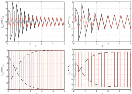
0 1 2 3 4 5 -2 -1.5 -1 -0.5 0 0.5 zp,1 and x p,1 t 0 1 2 3 4 5 -1 -0.5 0 0.5 1 1.5 zp,2 and x p,2 t
Figure 8.36: Positions (left) and velocities (right) of the Newton cradles for q(0, 0) = 0 0 1 2 3 4 5 -2 -1.5 -1 -0.5 0 0.5 zp,1 and x p,1 t 0 1 2 3 4 5 -0.2 0 0.2 0.4 0.6 0.8 1 1.2 zp,2 and x p,2 t
Figure 8.37: Positions (left) and velocities (right) of the Newton cradles for q(0, 0) = 1.
Figures 8.36 shows the response starting from q(0, 0) = 0, projected in the t direc-tion of the hybrid time domain. Since q(0, 0) = 0, the feedback stabilizer initially focuses on the real target. Mirroring allows to suitably treat the mismatch of the ordi-nary times when the impacts of z (red thin trace) and x (black bold trace) occur. For example, the first impact of the x cradle (black curve) occurs at (t1, 0)≈ (0.395, 0)
while the first impact of the z cradle (red curve) occurs at (t2, 1)≈ (0.435, 1). During
the flow between these two impacts, the control law tracks the mirrored target, namely q(t, 1) = 1 for all t∈ [t1, t2]. Figure 8.37 shows a second simulation starting from
q(0, 0) = 1. Clearly, the response of the z cradle (red curves) remains unchanged. Since q(0, 0) = 1, the initial target tracked by the controller is the mirrored one. This fact is evident in the both plots of Figure 8.37 which reveal that the tracker starts flowing in the opposite direction as compared to the previous case and after the first impact of the z cradle (red curve), occurring at ordinary time (t1, 0) = (0.435, 0), q
also the mismatch between the two subsequent impacts around ordinary time t ≈ 1.5. Also in this case the mirroring action allows to maintain the regularity of the transient response despite the impact mismatch.
8.4. Global tracking in planar triangles
One simplifying feature of the tracking algorithms of Sections 8.2 and 8.3 is that impacts always occur at a specific surface in the position subspace of the state space so that one can rely on a suitable mirror of the target with respect to that surface and recover the linear behavior of the error dynamics. This idea can be generalized to more complicated settings where impacts may occur on different surfaces, as long as each surface is associated to the correct mirrored image and suitable compositions of mirrors are performed when consecutive impacts on different surfaces are expe-rienced. The above intuitive behavior has been addressed in [FOR 11c] for several planar regions (or “billiards”) having special shapes. Moreover, for the case of rect-angular billiards, a comprehensive treatment is given in [FOR 11a]. In this section we revisit the results given in [FOR 11c, Section V.G] about dynamics restricted to subsets of the plane corresponding to equilateral triangles, and we show that global asymptotic tracking can be proven using the unified Lyapunov techniques given in Section 8.6.
8.4.1. The reference mass
We consider a tracking problem for a reference mass z moving in a planar region delimited by an equilateral triangle. The reference mass z = (zp, zv) ∈ #4is such
that its position sub-vector zpis confined to the region F ⊂ #2defined by
F = {s ∈ #2: ∀i ∈ I, .F
i, s− s◦/ ≤ 1}, (8.286)
with Fi ∈ #2, i ∈ {1, 2, 3} denoting the vectors characterizing each wall of the
triangle F and s◦∈ #2being a fixed point in the interior of the region characterizing
the position of the triangle in the plane (see Figure 8.38).
Following the approach in the previous section, we consider a quasi-linear refer-ence dynamics given by
˙z = Az + Bα(zp) z∈ Cz :=K ⊂ F × #2 (8.287)
where A := [0 1
0 0]⊗ I2, B := [01]⊗ I2, I2is the 2 × 2 identity matrix and α(zp) ∈
#2is a known nonlinear term that depends only on the position sub-vector z p. The
restriction of the flow and jump dynamics to the closed set K keeps the motion of the reference away from the “corners” of the triangular billiard, i.e. the points spsuch
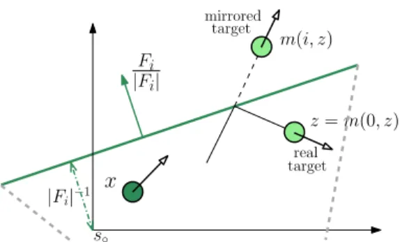
Fi |Fi| x |Fi|−1 m(i, z) mirrored target real target z= m(0, z) s◦
Figure 8.38: The triangular region F and the mirror of the target z with respect to one wall.
that .Fi, sp− s◦/ = .Fj, sp− s◦/ = 1 for i, j ∈ I, i += j. This assumption rules out
places where the impact dynamics may be a set valued map.
To ensure that the motion of the reference dynamics z = (zp, zv) is restricted to
the region F × #2, an impact occurs when the position z
pbelongs to the boundary
∂F of the triangle F and the velocity zvsatisfies .Fi, zv/ ≥ 0, for some i ∈ {1, 2, 3},
namely the mass bounces against the i-th wall represented by Fi. The impact on the
ith wall determines the inversion of the component of zvparallel to Fi(namely the
normal component to the wall). In [FOR 11b, FOR 11c, FOR 11a], such an impact was modeled by suitably combining two rotation matrices and the reflection matrix &1 0
0 −1
'
. Here, based on the derivations in [STR 03, page 220], we use the following simpler (and equivalent) formulation:
M (i) := I2− 2FiF T i
|Fi|2
, (8.288)
where I2is the identity matrix and |Fi| =
* FT
i Fi. Based on [STR 03, page 220], is
is easily verified that M (i) inverts the component of zvparallel to Fi. Thus, using the
definitions
c(i) := Fi· 2(1 + FiTs◦)/|Fi|2 (8.289a)
M (i) := I2⊗ M(i) (8.289b)
c(i) := & c(i)T 0
1×2 'T = [10]⊗ c(i) (8.289c)
m(i, z) := M (i)z + c(i) (8.289d)
the impact dynamics can be written compactly as z+= m(i, z) z∈ D(i)
where for each i ∈ {1, 2, 3}
Dz(i) := {z ∈ K : .Fi, zp− s◦/ = 1, .Fi, zv/ ≥ 0}
Dz := +
i∈{1,2,3}
D(i)z = ∂F × #2∩ K. (8.290b)
Finally, as in the previous sections, we augment the system dynamics with the aver-age dwell-time logic (8.253) having state σ and introduced in Section 8.2.2, to rule out Zeno solutions that occur when the reference mass impacts a wall Fiwith zero
orthog-onal component of zvto Fi(namely it slides along the wall). Similar to before, the
parameters of the dwell time logic do not appear in the tracking controller construc-tion but are essential for constructing the Lyapunov funcconstruc-tion establishing exponential convergence to zero of the error dynamics.
8.4.2. The controlled mass
Similar to the controlled Newton cradle of Section 8.3.2, the controlled mass shares the same dynamics as the reference mass but a force input u is available to suitably steer it towards the reference one during flows:
˙x = Ax + B(α(x) + u), x∈ Cx:=F × #2 (8.291a)
x+= m(i, x) x∈ Dx(i), i ={1, 2, 3}, (8.291b)
where for each i ∈ {1, 2, 3},
D(i)x := {x ∈ F × #2: .Fi, xp− s◦/ = 1, .Fi, xv/ ≥ 0}
Dx := +
i∈{1,2,3}
D(i)x = ∂F × #2. (8.291c)
Before introducing the mirrored references and the hybrid tracking law, it is conve-nient to proceed similarly to the Newton cradle by introducing an initial design for the control input u consisting in a linear error feedback plus cancellation of the nonlinear term α:
e = x− z
u = Ke− α(x) + α(z). (8.292)
Once again the gain is selected as
K := K⊗ I2= [k1k2]⊗ I2, (8.293)
where k1, k2guarantee that Acl = &k0 11k2
'
is a Hurwitz matrix. With this selection we have A + BK =&0 1
k1k2
'
⊗ I2, whose peculiar structure is exploited next in the
8.4.3. Using a family of mirrored references to design a hybrid stabilizer
Differently from the solutions in Sections 8.2.5 and 8.3.3 the triangle case can-not be solved by introducing a single mirror of the reference mass z. Indeed, since the triangular billiard has three walls, at least three mirrored images are necessary to generalize the hybrid tracking techniques of the previous sections. It turns out that 12 mirrored images will be necessary to solve our problem due to compositions of mirroring, as clarified below. Since we will introduce many mirrors in the sequel, the state variable q is not anymore a flag but it becomes a logic variable taking values in
Q = {0, 1, 2, 3, 21, 31, 12, 32, 13, 23, 121, 131, 232},
characterizing the real target (q = 0) and twelve suitable mirrors (see also Figures 8.38 and 8.39). This generalization has also been used in [FOR 11c, Section V.G] and an algebraic proof of the effectiveness of the scheme has been given. Here we rewrite the proof using graphical arguments which perhaps simplify the understanding of the rationale behind the hybrid scheme.
According to the scheme of Figure 8.39, for each z ∈ K (a possible one being suitably represented in the figure and comprising position and velocity), we define the mirrored references as m(0, z) = z, m(q, z) as specified in (8.289d) for q ∈ {1, 2, 3} and the remaining mirrors as the following compositions of the three basic mirrors (refer to Figure 8.39 for an intuitive understanding of each mirror):
m(21, z) = m(2, m(1, z)), m(31, z) = m(3, m(1, z)), m(12, z) = m(1, m(2, z)), m(32, z) = m(3, m(2, z)), m(13, z) = m(1, m(3, z)), m(23, z) = m(2, m(3, z)), m(121, z) = m(1, m(2, m(1, z))), m(131, z) = m(1, m(3, m(1, z))), m(232, z) = m(2, m(3, m(2, z))). (8.294)
Proceeding in ways similar to Section 8.3.3 we can then introduce the generalized error variable and the hybrid tracking law which coincides with equation (8.279) and is reproduced here for ease of presentation:
e = x− m(q, z)
u = Ke− α(x) + BTm(q, Bα(z)). (8.295)
While in the previous two sections the variable q was a flag that was easily toggled between 0 and 1 at each impact, for the triangular billiard case we need to suitably updating the logic variable q in such a way that a parallel result to Property 2 holds across jumps. To this aim, following the derivations in [FOR 11c, FOR 11a], we intro-duce two automata δz:Q×{1, 2, 3} → Q and δx:Q×{1, 2, 3} → Q which indicate
at each jump of z or x, respectively,10what should be the new value q+of the logic
10. Note that in [FOR 11a] the two automata are actually the same due to the special planar regions considered there.
1 1 1 1 2 2 2 2 Z m(0, z) 3 3 3 3 m(1, z) 2 Z 2 2 2 1 1 1 1 3 3 3 3 2 Z 2 2 2 1 1 1 1 3 3 3 3 2 Z 22 2 1 1 1 1 3 3 3 3 2 Z 2 2 2 1 1 1 1 3 3 3 3 2 Z 2 2 2 1 1 1 1 3 3 3 3 2 Z 22 2 1 1 1 1 3 3 3 3 2 Z 2 2 2 1 1 1 1 3 3 3 3 2 Z 2 2 2 1 1 1 1 3 3 3 3 2 Z 22 2 1 1 1 1 3 3 3 3 2 Z 2 2 2 1 1 1 1 3 3 3 3 2 Z 2 2 2 1 1 1 1 3 3 3 3 2 Z 2 2 2 1 1 1 1 3 3 3 3 m(2, z) m(12, z) m(21, z) m(121, z) m(31, z) m(32, z) X m(3, z) m(23, z) m(13, z) m(323, z) m(131, z) m(213, z) m(123, z) m(3121, z) 2 Z 2 2 2 1 1 1 1 3 3 3 3 2 Z 2 2 2 1 1 1 1 3 3 3 3 2 Z 2 2 2 1 1 1 1 3 3 3 3
F
1F
3F
2F
Figure 8.39: The triangular region of Section 8.4 and the twelve mirrored references. variable q. Determining suitable automata is the most difficult aspect of the construc-tion of this secconstruc-tion and will be discussed later in conjuncconstruc-tion with Property 3.
Summarizing, we can lump into a single hybrid dynamical system the dynamic equations (8.287), (8.290), (8.291), the controller (8.295), the dwell-time logic (8.253) and the dynamics of the automaton q to get the overall hybrid closed-loop system having flow dynamics given by (8.295) and
˙z = Az + Bα(z) ˙x = Ax + B(α(x) + u) ˙q = 0 ˙σ ∈ [0, ρ] (z, x, q, σ)∈ Cz× Cx× Q × [0, N]. (8.296)
Moreover an impact of the reference mass Z on the i-th wall is given by z+ = m(i, z) x+ = x q+ = δ z(q, i) σ+ = σ− 1 (z, x, q, σ)∈ D(i)z × (Cx∪ Dx)× Q × [1, N], (8.297)
while an impact of the controlled mass X on the i-th wall is described by z+ = z x+ = m(i, x) q+ = δ x(q, i) σ+ = σ− 1 (z, x, q, σ)∈ (Cz∪ Dz)× D(i)x × Q × [1, N]. (8.298)
Note that a synchronous impact of the reference and controlled masses is characterized by two consecutive jumps of the hybrid closed loop, given by either (8.297) followed by (8.298), or vice versa. Moreover, a simultaneous impact of the controlled mass on two walls (at a corner) may occur and is also characterized by two consecutive jumps of the hybrid closed loop, while a simultaneous impact of the reference mass on two walls (at a corner) is not possible because its motion is restricted to the closed set K which does not contain any corner.
The design of the hybrid tracking controller is completed by the selection of the automata δz, δx, which is carried out to ensure that whenever the reference mass z
or the controlled mass x experience an impact, the quantity eTP e involving the
gen-eralized error e in (8.295) does not increase, as long as P has a suitable structure (this parallels, e.g., the property in (8.283) for the Newton cradle). In particular, the automata δz, δxare determined graphically, based on the mirrored regions represented
in Figure 8.39, and corresponds to the following lookup tables:
q 0 1 2 3 21 31 12 32 13 23 121 131 232 δz(q, 1) 1 0 12 13 121 131 2 3 3 2 21 31 0 δz(q, 2) 2 21 0 23 1 3 121 232 1 3 12 0 32 δz(q, 3) 3 31 32 0 2 1 1 2 131 232 0 13 23 (8.299a) q 0 1 2 3 21 31 12 32 13 23 121 131 232 δx(q, 1) 1 0 21 31 2 3 121 2 131 3 12 13 0 δx(q, 2) 2 12 0 32 121 1 1 3 3 232 21 0 23 δx(q, 3) 3 13 23 0 1 131 2 232 1 2 0 31 32 (8.299b)
where each column represents q (the current value of the state q), each row represents a value of i (the wall that has been impacted by z or x), and the number in each cell indicates q+(the next value of the state q).
The construction of the automaton (8.299) is explained in the proof of the next property, which generalizes Properties 1 and 2 of the previous sections. Rather than
giving a full and formal proof of this property, we explain it graphically with reference to Figure 8.39. An alternative mathematical proof can be constructed following the guidelines in [FOR 11c, Section V.G].
Property 3 For any diagonal positive definite matrixP ∈ #2×2, defineP = P⊗ I 2.
Consider the hybrid closed loop (8.295),(8.296)–(8.298), (8.299). Then the jump map ensures that for alle in the jump set
(e+)TP e+≤ eTP e. (8.300)
Proof. (Graphical sketch). Let us first consider jumps of the z mass, namely lookup table in (8.299a) with reference to the mirrored images of Figure 8.39. First recall that |e|P = |x − m(q, z)|P denotes the (generalized) distance from
x (which is the green mass in the central region where q = 0) to the mirrored image of z corresponding to q (namely a specific column of the lookup table and a specific mirrored image of z in the corresponding region of Figure 8.39). When an impact of z occurs on wall i ∈ {1, 2, 3}, all the mirrored images impact on the edge corresponding to the mirror of the i-th wall, that is, the edge characterized by the small numbers i next to it. Since the impact reverses the orthogonal velocity to the wall, the italicized update rules in the lookup table (8.299a) ensure that q+= δ
z(q, i) characterizes the mirrored region on the opposite side of that edge.
Therefore, m(q+, z+) = m(q, z) and consequently e+= e, which in turns implies
|e+|
P =|e|P as to be proven.
The bold numbers in (8.299a) characterize a different situation where the mir-rored regions arising from the unfolding process of Figure 8.39 would move even beyond the set of white mirrors represented in the figure. Then it is possible to move back those regions closer to the central region (the actual billiard where q = 0) due to the special structure of P . Let us explain this in detail with refer-ence to the three pink regions in Figure 8.39 (one at the top and two at the bottom) which are remapped to regions closer to the center as shown by the red arrows. Since P = P ⊗ I2with P > 0 diagonal, then |e|P is the sum of four
indepen-dent non-negative terms, two coming from the difference of the speed of x and of the mirror m(q, z) of z and two coming from the position differences. Since each region is remapped to another mirror with the same orientation and the same horizontal position coordinate, then only the term that matters in the difference is the difference between the vertical displacements of x and m(q, z). Consider for example how q = 213 and q = 1 (lower left). Clearly, the vertical distance between x and m(1, z) is smaller than or equal to the triangle height h, while the vertical distance between x and m(123, z) is larger than or equal to h. Therefore, since the other three non-negative terms are the same, we get |e+|
P ≤ |e|P. This
(8.299a). Similar reasonings motivate the other bold numbers corresponding to the gray triangles in Figure 8.39. Note that in many cases this inequality is indeed strict and a (negative) jump of the error can be expected.
Let us now focus on a jump of x to explain the lookup table in (8.299b). Con-sider once again Figure 8.39 and notice that x always belongs to the central region. Therefore, an impact of x on the i-th wall, for some i ∈ {1, 2, 3}, corresponds to mirroring the velocity of x with respect to this wall. The update of q corresponding to the italicized numbers in (8.299b) is then carried out to ensure that the mirrored image of z jumps to the opposite side of the corresponding real wall, namely one among the orange (single lined), purple (double lined) or blue (triple lined) bound-aries in Figure 8.39. Since both x and m(q, z) jump with respect to the same mir-ror, their distance does not change and the error remains constant. In particular, it can be shown that |e+|
P =|M(i)(x − m(q, z))|P =|x − m(q, z)|M(i)P M(i) =
|x − m(q, z)|P, where the last step comes from similar calculations to those
car-ried out in (8.284). For illustration purposes, consider for example the case with q = 1 and when x impacts the second wall. Then Figure 8.39 suggests to mirror region “1” with respect to the purple double lined wall so to get q+ = 12. This
corresponds to the value at the second row of column “1” of table (8.299b). The bold numbers in table (8.299b) can be explained similarly to the previous case. As an example, consider q = 12 and impacting on the third wall, which would require mirroring the region “12” in Figure 8.39 into the pink region “123” at the bottom. Then, according to the bold 2 on the third row of column “12” of table (8.299b), we can select q+= δ
x(12, 3) = 2 and obtain|e+|P ≤ |e|P. !
Using the result of Property 3 we can prove the exponential convergence to zero of the generalized error, as stated in the following theorem which parallels Theorems 48 and 49 of the previous sections.
Theorem 50 There existsγ ≥ 1 and λ > 0 such that every hybrid solution ξ to the closed-loop system (8.295),(8.296)–(8.298), (8.299)) satisfies
|e(t, j)| ≤ γ exp(−λ(t + j))|e(0, 0)|. (8.301) Similar to the previous sections, we need to ensure that the exponential bound on the generalized error indeed is associated to some kind of (weakened) convergence of x to the actual mass z and not to one of its mirrors. The following proposition parallels Propositions 16 and 17 of the previous sections. Its intuitive implication is clarified in Figure 8.39, indeed since all the mirrors are outside the region q = 0 where the motion of x is constrained to evolve, the only possibility for x to flow with e = 0 is that it coincides with the real target mass z = m(0, z). This proof is sketched below.
Proposition 18 Consider any solutionξ to the hybrid closed-loop system (8.295), (8.296)–(8.298), (8.299)) starting from an initial condition satisfying e(0, 0) = 0. Thene(t, j) = 0 for all (t, j)∈ dom(e) and the solution cannot flow unless x(t, j) = z(t, j).
Proof. (Graphical sketch). Forward invariance of the set where e = 0 comes from the exponential bound (8.301). Refer to Figure 8.39 for the rest of the proof. Let us focus on the considered case when e(t, j) = 0, namely x(t, j) = m(q(t, j), z(t, j)), and the solution flows. Since the position xpof x = (xp, xv)
belongs to F and the position of all the mirrors of z with q += 0 do not belong to the interior of F, the only possibility for the solution to flow with e(t, j) = 0 and q(t, j)+= 0 is that xp(t, j) is at a boundary ofF and that q(t, j) ∈ {0, 1, 2, 3}. On
each boundary, the flow conditions (8.290b) and (8.291c) for x and z require that the speeds of z and x does not pierce the boundary. Then either q(t, j) = 0 and both speeds point inwards (and coincide because e(t, j) = 0) or q(t, j) ∈ {1, 2, 3} and the speed vector are coincident and parallel to the boundaries (the mass slides along one boundary). In this latter case, we have x(t, j) = z(t, j) even though
q(t, j)+= 0. !
8.4.4. Simulations
We illustrate the proposed approach by simulating the trajectories of the hybrid closed-loop system starting from the initial conditions zp(0, 0) = (−1, 0.3),
zv(0, 0) = (2, 2), xp(0, 0) = (−1.2, −0.5), xv(0, 0) = (0, 0) for the triangle
represented in Figure 8.40, which corresponds to: & F1 F2 F3 '= ! 0.7029 −0.7029 0 0.4058 0.4058 −1 " .
Figure 8.40 shows three trajectories starting from different initial conditions q(0, 0), namely starting from tracking of different mirrors. The left picture of the figure illus-trates the position trajectories of the two masses, while the right picture shows the evo-lution of the function |e(t, j)|P projected on the ordinary time direction t for the three
considered cases. In the left figure, the position of the real target is represented by the red dashed curve while the position of the controlled mass is represented in black when q(0, 0) = 0 (namely the tracking algorithm initially focuses on the real target mass z); it is represented in green when q(0, 0) = 1 (namely the tracking algorithm initially focuses on the target mass m(1, z) mirrored through the upper left wall); it is represented in blue when q(0, 0) = 3 (namely the tracking algorithm initially focuses on the target mass m(3, z) mirrored through the lower wall). Tracking performance and exponential decrease of the generalized error e can be appreciated for any initial condition, as guaranteed by the results of Theorem 50 and Proposition 18.
-2 -1 0 1 2 -1.5 -1 -0.5 0 0.5 1 1.5 2 2.5 3 zp,2 and x p,2 zp,1 and xp,1 0 0.5 1 1.5 2 2.5 0 5 10 15 20 25 |e|ο verline P t Trajectory of the target z Direct tracking (q(0,0)=0) Initially using the left mirror (q(0,0)=1) Initially using the bottom mirror (q(0,0)=3)
Figure 8.40: Trajectories of the hybrid tracking algorithm in a triangular region (left) and evolution of the generalized error (right).
8.5. Global state estimation onn-dimensional convex polyhedra
This section is apparently disconnected from the previous ones because it deals with state estimation rather than reference tracking and it also does not introduce any mirror to guarantee exponential convergence to zero of the error dynamics. Never-theless, the underlying technique remains the same, as it will be clear from the proof of the main result of this section, and the absence of mirrors arises from the strong simplification (that one can only use with observer dynamics) of not constraining the motion of both x and z into the confined region F.
8.5.1. The reference dynamics
We consider a state-estimation problem for a mass moving in an n-dimensional space, where we aim to make the observer state x ∈ #2nasymptotically converge to
the reference mass z ∈ #2nwhose position sub-vector belongs to a suitable
polyhe-dron F ⊂ #ndefined by
F = {s ∈ #n: ∀i ∈ I, .F
i, s− s◦/ ≤ 1}, (8.302)
with Fi ∈ #n, i ∈ I = {1, . . . , r} ⊂ N denoting the vectors characterizing each
wall of the n-dimensional polyhedral region F and s◦ ∈ #n being a fixed point in
the interior of the region. For example, if one moves s◦ while leaving Fi, i ∈ I
unchanged, then the shape of the region F remains unchanged and its position is moved accordingly. The algorithm proposed below generalizes the hybrid observer in [MEN 01c], where the case of one boundary I = {1} is considered in the planar case (that is, n = 2). Moreover, parallel results for the tracking case and for the case of an n-dimensional space have been discussed in [FOR 12]. The approach proposed here is simpler than the one in [FOR 12] because for the tracking case the controlled system
is forced to only lie in the region F. Instead, here we allow the observer dynamics to flow even for positions outside F and this greatly simplifies the approach. An alternative approach where the observer is constrained to not flow outside F has been discussed in [FOR 11a] for the case n = 2 and only for suitable polyhedral shapes. The core strategy presented here can be further generalized to convex sets F for which the normal vectors F (s) to a point s of the boundary ∂F are defined by a piecewise Lipschitz function F : ∂F → #2. We do not follow this generality here for reasons of
simplicity but the extension can be carried out in similar ways to the extension from the local results of [FOR 11b] to the local results of [FOR 11c].
Generalizing the approach of the previous section to an n-dimensional space, we consider a quasi-linear reference dynamics given by
˙z = Az + Bα(zp) z∈ Cz:=K ⊂ F × #n (8.303)
where A := [0 1
0 0]⊗ In, B := [01]⊗ In, and α(zp)∈ #nis a known nonlinear term
that depends only on the position sub-vector zp. We assume that the closed set K
restricts the motion of the reference away from the “corners” of the polyhedral region, i.e. the points spsuch that .Fi, sp− s◦/ = .Fj, sp− s◦/ = 1 for i, j ∈ I, i += j. This
assumption will avoid places where the impact dynamics may be a set valued map.
|Fi|−1 FT
i |Fi|
F
Figure 8.41: The polyhedral region F for the case n = 2 with the representation of the effect of an impact.
Similar to the technique adopted in Section 8.4.1, the motion of the reference dynamics z = (zp, zv) is restricted to the regionF ×#nby enforcing suitable impacts
on the mass when zpbelongs to the boundary ∂F of the polyhedron F and the
veloc-ity zvsatisfies .Fi, zv/ ≥ 0, for some i ∈ I. Once again, just as in (8.288), we use
describe an impact on the ith wall as:
M (i) := In− 2
FiFiT
|Fi|2, (8.304)
which inverts the component of zvorthogonal to Fi(recall that |Fi| =
* FT
i Fi). We
can then generalize the quantities introduced in (8.289) for the planar case as follows:
c(i) := Fi· 2(1 + FiTs◦)/|Fi|2 (8.305a)
M (i) := I2⊗ M(i) (8.305b)
c(i) := & c(i)T 0
1×n 'T= [10]⊗ c(i) (8.305c)
m(i, z) := M (i)z + c(i). (8.305d)
Then, based on (8.304), (8.305), the impact dynamics coincides with that of the planar case in (8.290) and corresponds to
z+= m(i, z) z∈ D(i)
z (8.306a)
where for each i ∈ I,
Dz(i) := {z ∈ K : .Fi, zp− s◦/ = 1, .Fi, zv/ ≥ 0}
Dz := +
i∈I
D(i)z = ∂F × #n∩ K.
(8.306b) The reference dynamics formulation is then concluded by adding the average dwell-time logic (8.253) having state σ and introduced in Section 8.2.2, to rule out Zeno solutions that occur when the reference mass impacts a wall Fi with zero parallel
component zvto Fi(namely it slides along the wall). Similar to before, the parameters
of the dwell time logic do not appear in the observer construction so that global results can be concluded.
8.5.2. The observer dynamics
Without impacts, following standard linear Luenberger constructions, we select the observer dynamics as a copy of the reference dynamics with a feedback injection term from the output error xp− zp= H(x− z), where H := [1 0]⊗ In:
˙x = Ax + Bα(zp) + LHe
where L = L ⊗ Inand L =
&!1
!2
'
is any output injection gain guaranteeing that the matrix Acl=
&!11
!20
'
is Hurwitz. As in the previous section, the specific selection of L guarantees that A + LC = Acl⊗ Inwhich is evidently a Hurwitz matrix because the
eigenvalues of X ⊗ Y are given by the products of each pair of eigenvalues of X and Y . Note also that A+ LC preserves the particular structure of the reference dynamics, which will be exploited in the hybrid reformulation of the observer algorithm.
Differently from the Newton’s cradle, the observer is not affected by impact phe-nomena. Therefore, the design of the jump dynamics is an extra degree of freedom in the hybrid reformulation of the observer.
8.5.3. Estimation by hybrid reformulation of the observer dynamics
The hybrid reformulation of the observer is based on two main features: (i) the observer is forced to jump whenever the reference dynamics jumps; (ii) when the reference dynamics impacts the boundary of F on the ith wall (namely it belongs to Dz(i)), the observer state is reset to x+= m(i, x). Imposing this specific reset rule on
the observer ensures the next property (we use properties from (8.305)): e+ = x+= z+= m(i, x)− m(i, z)
= M (i)(x− z) = M(i)e. (8.308)
Property (8.308) is fundamental to ensure that at each impact of the reference mass the observer is suitably reinitialized to account for the state change caused by the impact. This was the core motivation behind the approach of [MEN 01c] and is extended here to a broader class of problems. Note also that the approach is substantially different from the Newton’s cradle results of the previous section. Indeed there is no real need to constrain the motion of the observer in the region F and this greatly simplifies the analysis. More than that, the jump rule and jump set for the observer dynamics is an extra degree of freedom in the hybrid reformulation of the observer which is exploited to ensure the convenient linear behavior of e across jumps characterized in (8.308).
Selecting the observer flow dynamics in (8.307), forcing the observer to jump syn-chronously with the reference dynamics and with the jump rule described above, one gets the following overall hybrid closed-loop system (also incorporating the average dwell-time logic): ˙z = Az + Bα(zp) ˙x = Ax + LC(x− z) − Bα(zp) ˙σ ∈ [0, ρ] (z, x, σ)∈ Cz× #4× [0, N]. (8.309) z+ = m(i, z) x+ = m(i, x) σ = σ− 1. (z, x, σ)∈ D(i)z × #4× [1, N], (8.310)
for all i ∈ I. The hybrid dynamics (8.309), (8.310) characterizes a hybrid closed-loop system having flow set C = Cz× #4× [0, N] and jump set +
i∈I
Dz(i)× #4× [1, N]
where, due to the restriction of the z motion to the compact set K, the union is carried out among disjoint sets (in other words, no impacts on corners occur).
The hybrid observer proposed above is a straightforward hybrid extension of a continuous-time Luenberger observer, based on a suitable definition of the jump dynamics. In particular, in comparison to the hybrid controller for the tracking of the Newton’s cradle, there is no need to introduce any mirrored reference or any generalized error. This is a consequence of exploiting extra degrees of freedom for the continuous dynamics of the observer, whose position sub-vector is not constrained to lie in the polyhedral region F during transients. The generalized error may be introduced to formulate alternative observation laws where this constraint is enforced, as carried out in [FOR 11a] and [FOR 12]. Nevertheless the analysis in those cases is more involved and does not allow to achieve global results for a large class of polyhedral regions (which we obtain here).
Despite the absence of mirrored references, the rationale behind the stability anal-ysis that we carry out here is parallel to the one adopted in Section 8.3 and corresponds to exploiting the following property, which evidently parallels Property 2.
Property 4 For any matrixP ∈ #2×2, defineP = P ⊗ I
n. Consider the hybrid
closed loop (8.309)–(8.310) and the error variablee = x− z in (8.307). Then, for all e in the jump set of (8.309)–(8.310), we have
(e+)TP e+= eTP e. (8.311)
Proof.The proof relies upon (8.308) and similar calculations to those of (8.284) in the proof of Property 2. Indeed, from the definition of M (i) in (8.305b) and from the structure of P , we can use the properties of the Kronecker product to conclude that for each i ∈ I, M(i)P M(i) = P (recall also that M(i)M(i) = I for all i∈ I as shown in [STR 03, page 220]). Then the result follows by combining the
previous inequality with the identity in (8.308). !
Similar to the previous sections, the unifying Lyapunov result given in Sec-tion 8.6.1 combined with Property 4 allows us to state the following result establishing global exponential stability of the error dynamics. Its proof is given in Section 8.6.2.
Theorem 51 There existsγ > 1 and λ > 0 such that every hybrid solution ξ to the closed-loop system(8.309),(8.310) satisfies
|e(t, j)| ≤ γ exp(−λ(t + j))|e(0, 0)|, (8.312) wheree = x− z as defined in (8.307).
Note that since in the case study addressed in this section we did not introduce any mirrored reference, there is no need of proving a parallel result to that of Propo-sition 17. Indeed the conclusion of Theorem 51 implies that for any solution of the hybrid closed-loop system we have an exponential bound on e(t, j) = x(t, j)−z(t, j) which implies exponential convergence of the estimate x to the state z despite the impacts occurrence.
8.5.4. Simulations
We illustrate the proposed approach on a planar example (namely n = 2) where the polyhedron is a rectangle described by s◦= 0 and
& F1 F2 F3 F4 ':=1 4 ! 3 0 −3 0 0 4 −0 −4 " . (8.313)
We also consider a reference dynamics comprising a pair of double integrators, so that α(zp) = 0 for all zp.
Figure 8.42 shows the simulation results when the observer gain is selected as L = &−4
−4
'
, so that the eigenvalues of Aclare both in −2. The initial conditions of
the reference and observer dynamics is selected as z0 = [0.1 0.1 15 7]T and x0 =
[−0.5 0.1 −10 −3]T. The upper two plots of the figure, representing the horizontal and vertical positions projected in the t axis, respectively, show that the observer state (black trace) takes position values well outside the region F where the motion of the reference mass is constrained. This degree of freedom within the (virtual) observer dynamics is a key tool for establishing global results for such a general class of sys-tems. Alternative observation laws which exploit the mirroring technique of this chap-ter and constrain the motion of the observer state within the region F have also been proposed in recent years, but global results have only been proven for planar regions with special shapes, including rectangles. As an illustration of this, an observer with constrained motion has been given for this same example in [FOR 11a].
8.6. Proof of the main theorems
8.6.1. A useful Lyapunov result
In this section we introduce a Lyapunov result which establishes an exponential stability property that we will use for each of the proposed examples. This result,
0 1 2 3 4 5 -6 -4 -2 0 2 4 6 zp,1 and x p,1 t 0 1 2 3 4 5 -3 -2 -1 0 1 2 3 zp,2 and x p,2 t 0 1 2 3 4 5 -15 -10 -5 0 5 10 15 zv,1 and x v,1 t 0 1 2 3 4 5 -8 -6 -4 -2 0 2 4 6 8 zv,2 and x v,2 t
Figure 8.42: Simulation of the hybrid observer on a planar example. The upper graphs show the positions while the lower graphs show the velocity. Reference:red, observer: black.
suitably combined with the properties established in each one of the studied examples, will allow to prove the exponential properties stated in Theorems 48, 49, 51 which are yet to be proven. Each one of the above theorems will be proven in the next section based on the following lemma.
Lemma 12 Consider a hybrid dynamical system having state(e, ξ) and flow and jump setsCξ,Dξ, respectively. Assume that all solutions to this hybrid system satisfy
an average dwell-time condition, that the flow dynamics restricted toe corresponds to the following linear relation:
˙e = Acle, (e, ξ)∈ Cξ. (8.314)
Assume also that there exists a positive definite matrixP and a matrix H such that (H, Acl) is an observable pair and
eT(P Acl)e≤ −eTH T
He, ∀(e, ξ) ∈ Cξ, (8.315)
(e+)TP e+≤ eTP e, ∀(e, ξ) ∈ D
Then there existsγ ≥ 1 and λ > 0 such that all solutions to the hybrid dynamical system satisfy
|e(t, j)| ≤ γ exp(−λ(t + j))|e(0, 0)|. (8.317) Proof.The result is a direct consequence of [TEE 12, Theorem 2]. In particular, [TEE 12, Assumption 1] holds under the conditions of the lemma with x1 = e,
x2 = ξ, F1 = Acl, H1 = H, V (x) = V ((e, ξ)) = eTP e and µ = ∞. Then,
using the notation of [TEE 12, Theorem 2], we have |x|A = |e| and the global
exponential stability of A established by [TEE 12, Theorem 2] corresponds to the
exponential bound (8.317). !
8.6.2. Proofs of Theorems 48, 49, 50 and 51
In this section we prove the main theorems stated in each one of the examples addressed in this chapter. The proof of each statement will rely heavily on the Lya-punov result of Lemma 12. The motivation for grouping these proofs in a single sec-tion is to highlight the unified nature of the approach illustrated in this chapter which provides a different viewpoint on the result of our recent works [FOR 11b, FOR 11c, FOR 11a, FOR 12].
For the proofs of Theorems 48, 49, 50 and 51 below, we will first show that the generalized error dynamics satisfies (8.314) for a suitable Hurwitz matrix Acl. Then
a positive definite symmetric matrix P will be constructed to satisfy (8.315) and at the same time respect the structure required, respectively, in Properties 1, 2, 3, and 4. Indeed, each one of these properties ensures (in different ways) that equation (8.316). So that finally Lemma 12 can be applied to prove the corresponding theorem. The most relevant difference among the various examples probably resides on the cor-responding property. In particular, Property 1 ensures that eTP e remains constant
at each jump for any symmetric positive definite P , while Property 2 concludes the same result as long as P = P ⊗ I2. With Property 3 things are much more difficult
because P must be diagonal and even with such a constrained structure, one gets non-increase of eTP e even though there might be cases when the quantity experiences a
finite nonzero decrease. The diagonal structure of P also does not allow to obtain a “strict” decrease in (8.315) but the conditions of Lemma 12 are weak enough to allow for a non-full rank H in (8.315) as long as (H, Acl) is an observable pair. Finally,
Property 4 resembles the case of Property 2 with the similar structure P = P ⊗ Infor
P .
Proof of Theorem 48. We prove the theorem by showing that all the assumptions of Lemma 12 hold for the hybrid closed-loop system (8.256)-(8.258), (8.262)-(8.265).