Conventional and Reciprocal Approaches to the Forward and Inverse Problems of Electroencephalography

(1)

Conventional and Reciprocal Approaches to the

Forward and Inverse Problems of

Electroencephalography

by Stefan FINKE

Institut de génie biomédical Faculté de médecine

A thesis submitted in partial fulfillment of the requirements for the degree of Doctor of Philosophy in the Faculty of Graduate Studies

(Biomedical Engineering)

March, 2012

(2)

Cette thèse intitulée :

L’approche conventionnelle et réciproque aux problèmes direct et inverse de l’électroencéphalographie

présenté par : Stefan FINKE

a été évalué par un jury composé des personnes suivantes :

Frédéric LESAGE, président-rapporteur Ramesh M. GULRAJANI, directeur de recherche1

Pierre SAVARD, directeur de recherche Jean GOTMAN, codirecteur Vincent JACQUEMET, membre du jury

André ACHIM, examinateur externe

1_Décédé

(3)

Abstract

The inverse problem of electroencephalography (EEG) is the localization of current sources within the brain using surface potentials on the scalp generated by these sources. An inverse solution typically involves multiple calculations of scalp surface potentials, i.e., the EEG forward problem. To solve the forward problem, models are needed for both the underlying source configuration, the source model, and the surrounding tissues, the head model. This thesis treats two distinct approaches for the resolution of the EEG forward and inverse problems using the boundary-element method (BEM): the conventional approach and the reciprocal approach.

The conventional approach to the forward problem entails calculating the surface potentials starting from source current dipoles. The reciprocal approach, on the other hand, first solves for the electric field at the source dipole locations when the surface electrodes are reciprocally energized with a unit current. A scalar product of this electric field with the source dipoles then yields the surface potentials. The reciprocal approach promises a number of advantages over the conventional approach, including the possibility of increased surface potential accuracy and decreased computational requirements for inverse solutions.

In this thesis, the BEM equations for the conventional and reciprocal approaches are developed using a common weighted-residual formulation. The numerical implementation of both approaches to the forward problem is described for a single-dipole source model. A three-concentric-spheres head model is used for which analytic solutions are available. Scalp potentials are calculated at either the centroids or the vertices of the BEM discretization elements used. The performance of the conventional and reciprocal approaches to the forward problem is evaluated for radial and tangential dipoles of varying eccentricities and two widely different skull conductivities.

We then determine whether the potential advantages of the reciprocal approach suggested by forward problem simulations can be exploited to yield more accurate inverse solutions. Single-dipole inverse solutions are obtained using simplex minimization for both the conventional and reciprocal approaches, each with centroid and

(4)

vertex options. Again, numerical simulations are performed on a three-concentric-spheres model for radial and tangential dipoles of varying eccentricities. The inverse solution accuracy of both approaches is compared for the two different skull conductivities and their relative sensitivity to skull conductivity errors and noise is assessed.

While the conventional vertex approach yields the most accurate forward solutions for a presumably more realistic skull conductivity value, both conventional and reciprocal approaches exhibit large errors in scalp potentials for highly eccentric dipoles. The reciprocal approaches produce the least variation in forward solution accuracy for different skull conductivity values. In terms of single-dipole inverse solutions, conventional and reciprocal approaches demonstrate comparable accuracy. Localization errors are low even for highly eccentric dipoles that produce large errors in scalp potentials on account of the nonlinear nature of the single-dipole inverse solution. Both approaches are also found to be equally robust to skull conductivity errors in the presence of noise.

Finally, a more realistic head model is obtained using magnetic resonance imaging (MRI) from which the scalp, skull, and brain/cerebrospinal fluid (CSF) surfaces are extracted. The two approaches are validated on this type of model using actual somatosensory evoked potentials (SEPs) recorded following median nerve stimulation in healthy subjects. The inverse solution accuracy of the conventional and reciprocal approaches and their variants, when compared to known anatomical landmarks on MRI, is again evaluated for the two different skull conductivities. Their respective advantages and disadvantages including computational requirements are also assessed.

Once again, conventional and reciprocal approaches produce similarly small dipole position errors. Indeed, position errors for single-dipole inverse solutions are inherently robust to inaccuracies in forward solutions, but dependent on the overlapping activity of other neural sources. Against expectations, the reciprocal approaches do not improve dipole position accuracy when compared to the conventional approaches. However, significantly smaller time and storage requirements are the principal advantages of the reciprocal approaches. This type of localization is potentially useful in the planning of neurosurgical interventions, for example, in patients with refractory focal epilepsy in whom EEG and MRI are often already performed.

(5)

Keywords: Electroencephalography, weighted-residual formulation, boundary-element

method, equivalent current dipole, forward problem, reciprocity, inverse problem, source localization, somatosensory evoked potential.

(6)

Résumé

Le problème inverse en électroencéphalographie (EEG) est la localisation de sources de courant dans le cerveau utilisant les potentiels de surface sur le cuir chevelu générés par ces sources. Une solution inverse implique typiquement de multiples calculs de potentiels de surface sur le cuir chevelu, soit le problème direct en EEG. Pour résoudre le problème direct, des modèles sont requis à la fois pour la configuration de source sous-jacente, soit le modèle de source, et pour les tissues environnants, soit le modèle de la tête. Cette thèse traite deux approches bien distinctes pour la résolution du problème direct et inverse en EEG en utilisant la méthode des éléments de frontières (BEM): l’approche conventionnelle et l’approche réciproque.

L’approche conventionnelle pour le problème direct comporte le calcul des potentiels de surface en partant de sources de courant dipolaires. D’un autre côté, l’approche réciproque détermine d’abord le champ électrique aux sites des sources dipolaires quand les électrodes de surfaces sont utilisées pour injecter et retirer un courant unitaire. Le produit scalaire de ce champ électrique avec les sources dipolaires donne ensuite les potentiels de surface. L’approche réciproque promet un nombre d’avantages par rapport à l’approche conventionnelle dont la possibilité d’augmenter la précision des potentiels de surface et de réduire les exigences informatiques pour les solutions inverses.

Dans cette thèse, les équations BEM pour les approches conventionnelle et réciproque sont développées en utilisant une formulation courante, la méthode des résidus pondérés. La réalisation numérique des deux approches pour le problème direct est décrite pour un seul modèle de source dipolaire. Un modèle de tête de trois sphères concentriques pour lequel des solutions analytiques sont disponibles est utilisé. Les potentiels de surfaces sont calculés aux centroïdes ou aux sommets des éléments de discrétisation BEM utilisés. La performance des approches conventionnelle et réciproque pour le problème direct est évaluée pour des dipôles radiaux et tangentiels d’excentricité variable et deux valeurs très différentes pour la conductivité du crâne.

(7)

suggérés par les simulations du problème direct peuvent êtres exploités pour donner des solutions inverses plus précises. Des solutions inverses à un seul dipôle sont obtenues en utilisant la minimisation par méthode du simplexe pour à la fois l’approche conventionnelle et réciproque, chacun avec des versions aux centroïdes et aux sommets. Encore une fois, les simulations numériques sont effectuées sur un modèle à trois sphères concentriques pour des dipôles radiaux et tangentiels d’excentricité variable. La précision des solutions inverses des deux approches est comparée pour les deux conductivités différentes du crâne, et leurs sensibilités relatives aux erreurs de conductivité du crâne et au bruit sont évaluées.

Tandis que l’approche conventionnelle aux sommets donne les solutions directes les plus précises pour une conductivité du crâne supposément plus réaliste, les deux approches, conventionnelle et réciproque, produisent de grandes erreurs dans les potentiels du cuir chevelu pour des dipôles très excentriques. Les approches réciproques produisent le moins de variations en précision des solutions directes pour différentes valeurs de conductivité du crâne. En termes de solutions inverses pour un seul dipôle, les approches conventionnelle et réciproque sont de précision semblable. Les erreurs de localisation sont petites, même pour des dipôles très excentriques qui produisent des grandes erreurs dans les potentiels du cuir chevelu, à cause de la nature non linéaire des solutions inverses pour un dipôle. Les deux approches se sont démontrées également robustes aux erreurs de conductivité du crâne quand du bruit est présent.

Finalement, un modèle plus réaliste de la tête est obtenu en utilisant des images par resonace magnétique (IRM) à partir desquelles les surfaces du cuir chevelu, du crâne et du cerveau/liquide céphalorachidien (LCR) sont extraites. Les deux approches sont validées sur ce type de modèle en utilisant des véritables potentiels évoqués somatosensoriels enregistrés à la suite de stimulation du nerf médian chez des sujets sains. La précision des solutions inverses pour les approches conventionnelle et réciproque et leurs variantes, en les comparant à des sites anatomiques connus sur IRM, est encore une fois évaluée pour les deux conductivités différentes du crâne. Leurs avantages et inconvénients incluant leurs exigences informatiques sont également évalués.

(8)

Encore une fois, les approches conventionnelle et réciproque produisent des petites erreurs de position dipolaire. En effet, les erreurs de position pour des solutions inverses à un seul dipôle sont robustes de manière inhérente au manque de précision dans les solutions directes, mais dépendent de l’activité superposée d’autres sources neurales. Contrairement aux attentes, les approches réciproques n’améliorent pas la précision des positions dipolaires comparativement aux approches conventionnelles. Cependant, des exigences informatiques réduites en temps et en espace sont les avantages principaux des approches réciproques. Ce type de localisation est potentiellement utile dans la planification d’interventions neurochirurgicales, par exemple, chez des patients souffrant d’épilepsie focale réfractaire qui ont souvent déjà fait un EEG et IRM.

Mots-clés: Électroencéphalographie, méthode des résidus pondérés, méthode des

éléments de frontières, dipôle de courant équivalent, problème direct, réciprocité, problème inverse, localisation de source, potentiel évoqué somatosensoriel.

(9)

List of Tables

Table 4.1. The number of elements and nodes, the average element edge lengths, and the average surface radii in mm are given for Level 1, 2, 3, and Q discretizations for the scalp surface as well as for discretizations for the skull and brain/CSF surfaces of Subjects A, B, and C (see Figure 4.1). Discretization elements are triangles and nodes are triangle vertices except for Level Q where elements also include curvilinear quadrilaterals (i.e., one at each electrode site considered) and nodes also include quadrilateral vertices (i.e., nine per quadrilateral). Level 1, Level 2, and Level 3 discretizations for the scalp surface are used with the CC, CV, and RC approaches while Level Q discretization for the scalp surface is used with the RV approach. All approaches use identical discretizations for the skull and brain/CSF surfaces of each subject. All radii are calculated in relation to the center of the innermost brain/CSF volume conductor. 84

Table 4.2. Maximum and average electrode localization errors in mm for the CC, CV, RC, and RV approaches for Level 1, 2, 3, and Q discretizations for the scalp surface of Subjects A, B, and C. Level 1, Level 2, and Level 3 discretizations for the scalp surface are used with the CC, CV, and RC approaches while Level Q discretization for the scalp surface is used with the RV approach. 86

Table 4.3. Relative-difference measure (RDM) in % of N20-P20 SEP inverse solutions for right and left median nerve stimulation of Subjects A, B, and C. Level 1, Level 2, and Level 3 discretizations for the scalp surface are used by the CC, CV, and RC approaches while Level Q discretization for the scalp surface is used by the RV approach. 91

Table 4.4. Dipole position error in mm of N20-P20 SEP inverse solutions for right and left median nerve stimulation of Subjects A, B, and C compared to the nearest point of the corresponding primary sensory hand areas identified on MRI. Level 1, Level 2, and Level 3 discretizations for the scalp surface are used by the CC, CV, and RC approaches while

(13)

Level Q discretization for the scalp surface is used by the RV approach. A position error of zero signifies that the dipole is located within the primary sensory hand area. 92

Table 4.5. Position error tolerance in mm of N20-P20 SEP inverse solutions for right and left median nerve stimulation of Subjects A, B, and C. Position error tolerance is defined as the greatest improvement in dipole position error by a non-minimum RDM solution when compared to the dipole position error of the minimum RDM solution (see text). Level 1, Level 2, and Level 3 discretizations for the scalp surface are used by the CC, CV, and RC approaches while Level Q discretization for the scalp surface is used by the RV approach. Note that if the minimum RDM dipole position error is zero (see Table

4.4) then no further improvement is possible and the position error tolerance is also zero. 98

(14)

List of Figures

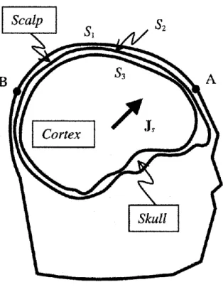
Figure 2.1. A three-surface head model with a source current dipole

!

J_s and surface

electrodes A and B. 27

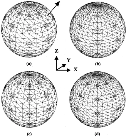
Figure 2.2. (a), (b) Sphere discretizations used with the CC, CV, and RC approaches. There are 1572 triangles per surface in (a) and 2228 in (b). The 45° axis along which the dipole is moved is shown dotted in (a). (c), (d) Sphere discretization with the RV approach. In addition to 42 curvilinear quadrilaterals, there are 1824 triangles in (c) and 2480 triangles in (d). See text for additional details. 41

Figure 2.3. Relative difference measures plotted against dipole eccentricity for radial (solid line) and tangential (dotted line) dipoles. Results for both CC (circles) and CV (triangles) approaches are depicted. Relative skull conductivity was 1/80 in (a) and 1/15

in (b). 43

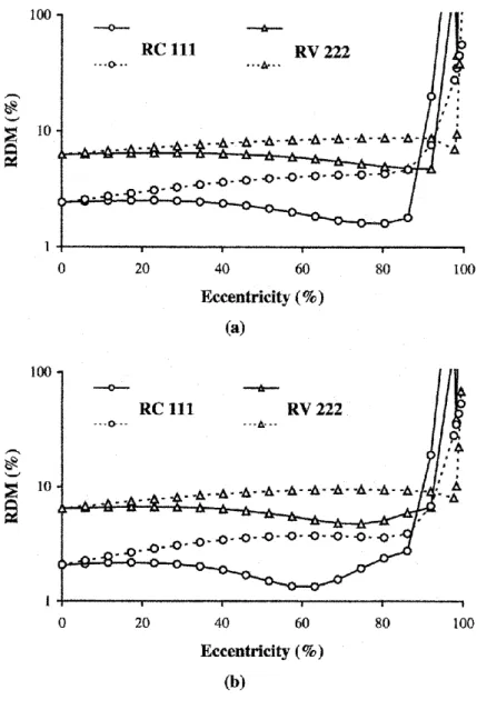
Figure 2.4. Relative difference measures plotted against dipole eccentricity for radial (solid line) and tangential (dotted line) dipoles. Results for both RC (circles) and RV (triangles) approaches are depicted. Relative skull conductivity was 1/80 in (a) and 1/15

in (b). 44

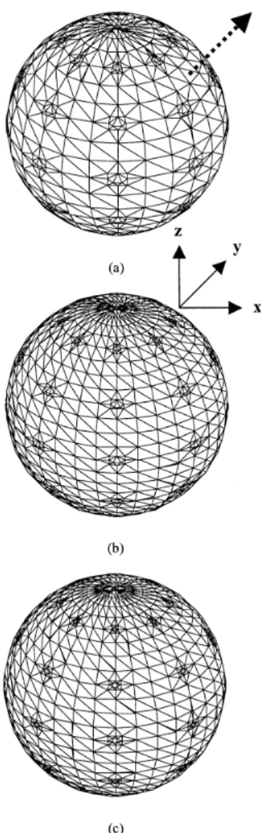
Figure 3.1. Level 1 sphere discretization is shown in (a), and level 2 sphere discretizations are shown in (b) and (c). There are 1572 triangles per sphere in (a), and 2228 triangles per sphere in (b). In addition to the 42 curvilinear quadrilaterals, there are 2480 triangles in (c). The CC and RC approaches use sphere (a), the CV approach uses sphere (b), and the RV approach sphere (c). The axis along which the source dipole is moved is shown by the arrow in (a). To give a quantitative idea of the discretizations, at the equator in (c), the quadrilaterals are of 4.3-mm width and 2.9-mm height for the outermost sphere of radius 10 cm, 4.0-mm width and 2.7-mm height for the middle sphere of radius 9.2 cm, 3.8-mm width and 2.5-mm height for the innermost sphere of

(15)

radius 8.7 cm. Coordinate axes are as shown. 54

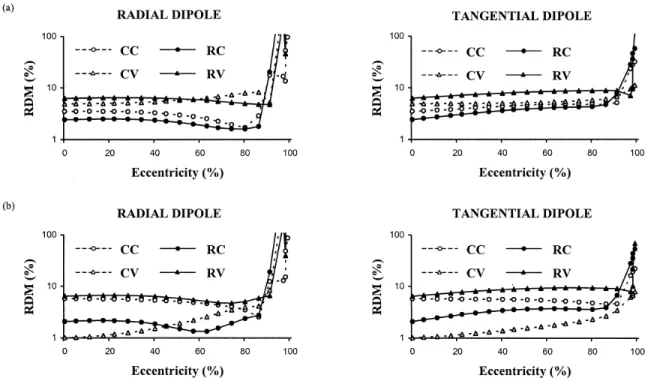
Figure 3.2. RDM of the forward problem versus dipole eccentricity for radial and tangential dipoles (maximum eccentricity is 8.65 cm). Relative skull conductivity is 1/80 in (a) and 1/15 in (b). Results for conventional approaches (CC and CV) are shown using dashed lines and those for reciprocal approaches (RC and RV) are shown using solid lines. The CC and RC approaches (circles) use level 1 discretizations for all three spheres, while the CV and RV approaches (triangles) use level 2 discretizations for all

spheres. 58

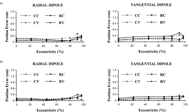
Figure 3.3. Dipole position error versus dipole eccentricity for radial and tangential dipoles in the absence of measurement noise (maximum eccentricity is 8.5 cm). Relative skull conductivity is 1/80 in (a) and 1/15 in (b). Results for conventional approaches (CC and CV) are shown using dashed lines and those for reciprocal approaches (RC and RV) are shown using solid lines. The CC and RC approaches (circles) use level 1 discretizations for all three spheres, while the CV and RV approaches (triangles) use level

2 discretizations for all spheres. 59

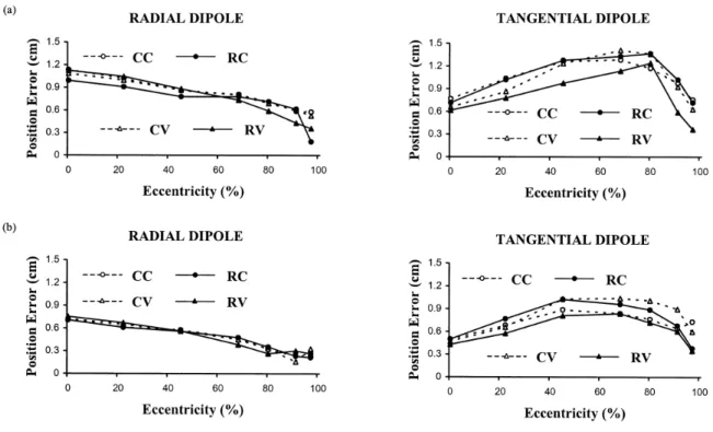
Figure 3.4. Dipole position error versus dipole eccentricity for radial and tangential dipoles in the presence of 20% noise (maximum eccentricity is 8.5 cm). Relative skull conductivity is 1/80 in (a) and 1/15 in (b). The format is the same as in Figure 3.3. 60

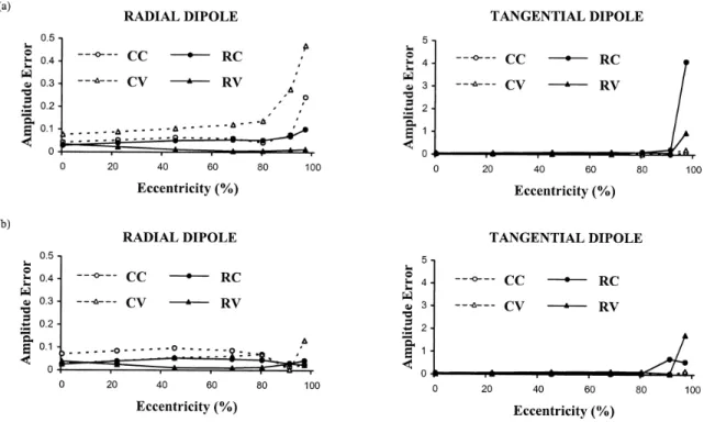
Figure 3.5. Dipole amplitude error versus dipole eccentricity for radial and tangential dipoles in the presence of 20% noise (maximum eccentricity is 8.5 cm). Relative skull

conductivity is 1/80 in (a) and 1/15 in (b). The format is the same as in Figure 3.3. Note, however, that the graphs for radial and tangential dipoles have different vertical scales.

61

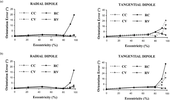
Figure 3.6. Dipole orientation error versus dipole eccentricity for radial and tangential dipoles in the presence of 20% noise (maximum eccentricity is 8.5 cm). Relative skull conductivity is 1/80 in (a) and 1/15 in (b). The format is the same as in Figure 3.3. Note,

(16)

however, that the graphs for radial and tangential dipoles have different vertical scales. 62

Figure 3.7. Dipole position error versus dipole eccentricity for radial dipoles in the presence of 20% noise (maximum eccentricity is 8.5 cm). Each graph refers to a particular inverse solution, with conventional approaches shown using hollow symbols and reciprocal approaches using full symbols. Relative skull conductivity was 1/15 in all inverse solutions, but a relative skull conductivity of

!

1/15

(

)

± 25% was assumed in computing the input analytic potentials. The CC and RC approaches (circles) use level 1 discretizations for all three spheres, while the CV and RV approaches (triangles) use level

2 discretizations for all spheres. 63

Figure 3.8. Dipole position error versus dipole eccentricity for tangential dipoles in the presence of 20% noise (maximum eccentricity is 8.5 cm). Relative skull conductivity was 1/15 in all inverse solutions, but a relative skull conductivity of

!

1/15

(

)

± 25% was assumed in computing the input analytic potentials. The format is the same as in Figure

3.7. 64

Figure 3.9. Diagram of the dipole position error versus RDM for each of the ten simplex trials used to locate a tangential dipole at an eccentricity of 8.5 cm (97.7%) with a relative skull conductivity of 1/80. The inverse solution was computed with the CV approach, in the presence of 20% noise but with no error in skull conductivity. All simplexes converged, but three clusters (A, B, and C) may be identified. A magnification of cluster A is provided. The minimum RDM solution is identified with a larger triangle, and yields a position error of 6.27 mm. Other solutions in cluster A yielded slightly smaller position errors, but the lowest position error was obtained by the single point corresponding to cluster B, which yielded a position error of 6.17 mm. 65

Figure 3.10. RDM plotted against trial dipole eccentricity along

!

x,

!

y , and

!

z axes, for the

noiseless case (a) and for 20% Gaussian measurement noise (b). The source dipole is a centric radial dipole, oriented along the direction shown by the dotted arrow in Figure

(17)

3.1(a). A three-sphere model with relative skull conductivity of 1/15 was used. Analytic surface potentials were computed from this source dipole for the noiseless case (a), and contaminated with 20% noise (b), to yield the so-called measured potentials

!

ˆ

u _i. The RDM is evaluated from (5) with the numerical potentials

!

u_i, corresponding to an optimum dipole placed at trial positions at 0.5-cm intervals along the axes, computed with transfer matrices

!

T determined by the RV approach. The minimum RDM point is

identified with a larger symbol. 68

Figure 4.1. A shows discretizations obtained from CURRY for the scalp (i), skull (ii), and brain/CSF surfaces (iii) of Subject A. Projected electrode sites including the reference electrode Cz are shown with black circles at triangle vertices in A(i). B illustrates refinement (solid lines) of the discretization in A(i) around electrode 94 for the scalp surface (dashed lines) of the same subject. In B(i) the electrode site corresponds to the innermost triangle centroid, in B(ii) the electrode site corresponds to the quadrilateral center, and in B(iii) the electrode site corresponds to the innermost triangle vertex. Level 1 (shown in A(i)), Level 2 (shown in B(i)), and Level 3 (shown in B(iii)) discretizations for the scalp surfaces are used with the CC, CV, and RC approaches while Level Q (shown in B(ii)) discretization for the scalp surface is used with the RV approach. All approaches use discretizations for the skull and brain/CSF surfaces shown in A(ii) and A(iii), respectively. See Table 4.1 and text for additional details. 83

Figure 4.2. Axial (a) and sagittal (b) slices through the left primary sensory hand area (shown in grey) identified on MRI for Subject A. The characteristic knob-like structure arising from the posterior wall of the precentral gyrus (PrCG) is shaped like an Ω in the axial (a) plane and like a hook in the sagittal (b) plane and corresponds to the left primary motor hand area. The primary sensory hand area is adjacent to the primary motor hand area in the posterior bank of the central sulcus (CS) in the postcentral gyrus (PoCG). Note that the scales in (a) and (b) are different. Images are generated using NeuroLens. 87

Figure 4.3. Average-reference measured and calculated N20-P20 SEPs for right and left median nerve stimulation of Subjects A, B, and C visualized from directly above each

(18)

subject (i.e., reference electrode Cz). Calculated scalp potential distributions are shown for the CC (Level 1), CV (Level 1), RC (Level 2), and RV (Level Q) approaches. CC, CV, and RC calculated potential distributions for other discretizations of the scalp surface (not shown) are similar in appearance to those shown for each stimulation study. Note that scale ranges for different potential distributions are not identical. Images are generated using EEGLAB in MATLAB (Mathworks, Natick, MA). 90

Figure 4.4. N20-P20 SEP inverse dipole solutions for right and left median nerve stimulation of Subject A for the CC (Level 1), CV (Level 1), RC (Level 2), and RV (Level Q) approaches compared to the nearest point of the corresponding primary sensory hand areas identified on MRI. Primary sensory hand areas are shown in grey. Red, blue, green, and yellow represent the CC, CV, RC, and RV approaches, respectively. Arrows depict inverse dipole solutions and dashed lines depict dipole position errors projected onto the image plane. Shown are axial (top), sagittal (middle), and coronal (bottom) slices through the median coordinates of the primary sensory hand area points nearest to the inverse dipole solutions. L indicates the left, F the front, and T the top of the subject’s head. Note that the distances shown are 2.3 times the actual values. Images are generated

using NeuroLens. 94

Figure 4.5. N20-P20 SEP inverse dipole solutions for right and left median nerve stimulation of Subject B for the CC (Level 1), CV (Level 1), RC (Level 2), and RV (Level Q) approaches compared to the nearest point of the corresponding primary sensory hand areas identified on MRI. Primary sensory hand areas are shown in grey. Red, blue, green, and yellow represent the CC, CV, RC, and RV approaches, respectively. Arrows depict inverse dipole solutions and dashed lines depict dipole position errors projected onto the image plane. Shown are axial (top), sagittal (middle), and coronal (bottom) slices through the median coordinates of the primary sensory hand area points nearest to the inverse dipole solutions. L indicates the left, F the front, and T the top of the subject’s head. Note that the distances shown are 2.3 times the actual values. Images are generated

(19)

Figure 4.6. N20-P20 SEP inverse dipole solutions for right and left median nerve stimulation of Subject C for the CC (Level 1), CV (Level 1), RC (Level 2), and RV (Level Q) approaches compared to the nearest point of the corresponding primary sensory hand areas identified on MRI. Primary sensory hand areas are shown in grey. Red, blue, green, and yellow represent the CC, CV, RC, and RV approaches, respectively. Arrows depict inverse dipole solutions and dashed lines depict dipole position errors projected onto the image plane. Shown are axial (top), sagittal (middle), and coronal (bottom) slices through the median coordinates of the primary sensory hand area points nearest to the inverse dipole solutions. L indicates the left, F the front, and T the top of the subject’s head. Note that the distances shown are 2.3 times the actual values. Images are generated

using NeuroLens. 96

Figure 4.7. Dipole position error in mm versus relative-difference measure (RDM) in % of N20-P20 SEP inverse solutions for right and left median nerve stimulation of Subjects A, B, and C. Plotted points are shown for the CC (Level 1), CV (Level 1), RC (Level 2), and RV (Level Q) approaches. The highest RDM values are for right median nerve stimulation of Subject B and the lowest RDM values are for right median nerve stimulation of Subject C. The largest position errors are for right and left median nerve stimulation of Subject B and the smallest position errors are for right median nerve stimulation of Subject A. 97

(20)

List of Symbols and Acronyms

3D Three-dimensional

AEP Auditory evoked potential

BEM Boundary-element method

BESA Brain Electrical Source Analysis

CC Conventional centroid

CIHR Canadian Institutes of Health Research

CRIUGM Centre de recherche de l’Institut universitaire de gériatrie de Montréal

CSF Cerebrospinal fluid

CSSD Common spatial subspace decomposition

CT Computed tomography

CURRY Current Reconstruction and Imaging

CV Conventional vertex

DSL Dipole source localization

(21)

EEG Electroencephalography

EEGLAB Electroencephalography Laboratory

EGI Electrical Geodesics Incorporated

EP Evoked potential

ERP Event-related potential

FDM Finite-difference method

FEM Finite-element method

FLASH Fast low-angle shot

fMRI Functional magnetic resonance imaging

FOV Field of view

FRQS Fonds de recherche du Québec – Santé

FS Fat suppression

GFP Global field power

HPC High-performance computing

ICA Independent component analysis

(22)

LCR Liquide céphalorachidien

LORETA Low-resolution electromagnetic tomography

MATLAB Matrix Laboratory

MEG Magnetoencephalography

MNI Montreal Neurological Institute

MRI Magnetic resonance imaging

MUSIC Multiple signal classification

N20-P20 Negative and positive potential peaks measured at 20 ms post median nerve stimulation

NSERC Natural Sciences and Engineering Research Council of Canada

PAL Pre-auricular left

PAR Pre-auricular right

PCA Principal-component analysis

PET Position emission tomography

RC Reciprocal centroid

(23)

R-MUSIC Recursive multiple signal classification

RQCHP Réseau québécois de calcul de haute performance

RV Reciprocal vertex

SEP Somatosensory evoked potentials

SI Primary somatosensory cortex

SNR Signal-to-noise ratio

SPECT Single-position emission tomography

STDM Spatio-temporal dipole modeling

SVD Singular value decomposition

TE Echo time

TR Repetition time

(24)

(25)

Acknowledgements

Special thanks to the following individuals for all their invaluable assistance:

Marie-Claire ALBANESE Andrew BAGSHAW Michel BÉLAND Louise BÉLANGER Christian BÉNAR André BLEAU Natalie CHANG Philippe COMTOIS Laurent DESCARRIES Anne-Sophie DUBARRY Bruno DUBÉ Emma DUERDEN Michael FERREIRA Sukhi GREWAL Christophe GROVA Colin HAWCO Yann HENZEL Peter JOHNSTON Syma KHAN Ping Hei LAM Nadine LEBLANC Robert LEBLANC Richard LEFEBVRE Frédéric LESAGE Jean-Marc LINA Bernard LORAZO

(26)

Kristina MARTINU Pierre MATHIEU Sylvain MILOT Tomáš PAUS Linda PELLETIER Pierre RAINVILLE Gonzalo REYES Bart VANRUMSTE Alain VINET

(27)

Chapter 1 Introduction

1.1 Reciprocity

The well-known theorem of reciprocity in electromagnetics was introduced by Helmholtz in 1853 (Helmholtz, 1853) and applied to electroencephalography (EEG) by Rush and Driscoll (1969) and Nunez (1981) for electrode sensitivity. It has since been used to compare sensitivity distributions for EEG and magnetoencephalography (MEG) (Malmivuo and Plonsey, 1995; Malmivuo et al., 1997). The reciprocity theorem has also been invoked to calculate potentials on a homogenous sphere (Brody et al., 1973), and on numerical head models employing the boundary-element method (BEM) (Fletcher et al., 1995; Finke, 1998), the finite-difference method (FDM) (Laarne, 2000; Laarne et al., 2000; Vanrumste et al., 2000; Vanrumste, 2001; Vanrumste et al., 2001; Hallez et al., 2005), and the finite-element method (FEM) (Weinstein et al., 2000). Riera and Fuentes (1998) presented an alternative reciprocal formulation for the BEM in terms of current fluxes.

The lead field is the electric field in a volume conductor generated by injecting unit current into a lead (i.e., an electrode pair on that volume conductor). According to the theorem of reciprocity, the electric field produced in this manner entirely determines the sensitivity distribution of the lead in question. This lead field therefore characterizes a type of electrical access of an electrode pair to any point in the volume conductor. It is only dependent on the geometric and electrical properties of the volume conductor, which is assumed passive in this case (i.e., containing no current sources), in addition to the position of the lead or electrode pair. Note that the electric field is the current density divided by the local conductivity (i.e., the electric field is directly proportional to the current density in a homogenous volume conductor model) and the lead field is the electric field normalized by the amplitude of the injected current (i.e., the lead field is equal to the electric field when unit current is injected).

The lead field defines the sensitivity of the electrode pair used for current injection and withdrawal to sources at a particular location in the volume conductor. In

(28)

other words, knowledge of the electric field (or current density) throughout a volume conductor due to current injection across two stimulating electrodes fully describes how those same electrodes measure potentials due to sources anywhere in the volume conductor when they are used as EEG recording electrodes. The potential difference between these two electrodes generated by a current dipole (see Section 1.4) at the source location can be obtained by forming the scalar product of this electric field and the dipole moment. Calculating scalp potentials in this manner is called the lead-field or reciprocal approach and represents an alternative formulation for solving the EEG forward problem.

1.2 Forward Solutions

EEG deals with potentials recorded on the scalp resulting from the electrical activity of brain cells or neurons (see Section 1.4). The EEG forward problem generally refers to the determination of potential distributions resulting from known neural sources in a given volume conductor head model (Hallez et al., 2007). The mathematical formulation of the forward problem is obtained from Poisson’s equation (Plonsey, 1969; Johnson, 1995; Gulrajani, 1998). Forward solutions can be used to compare scalp potentials (e.g., for different approaches to the forward problem or for calculated and measured potentials) (Fletcher et al., 1995, Finke, 1998) and for source imaging (e.g., cortical potential calculations) (Gevins et al., 1994; He et al., 1999). They are also usually required for EEG inverse solutions (Mosher et al., 1999b) and their validity is therefore presumed critical for accurate source localization (see Section 1.3).

Potential distributions can be calculated using analytic equations when volume conductors consisting of simple geometrical shapes such as spheres are considered (Rush and Driscoll, 1969; Ary et al., 1981). These analytical approaches were mostly used when computational capacity was more restricted (Gaumond et al., 1983; Gulrajani et al., 1984; Cuffin et al., 1985), but they are still currently employed especially as a reference for validation of numerical approaches (Thevenet et al., 1991; Yan et al., 1991; Eshel et al., 1995; Finke, 1998; Vanrumste et al., 2000) that may also be used on more realistically-shaped head models (see Section 1.5).

(29)

With the boundary-element method (BEM) for solving Poisson’s equation numerically, only tissue boundaries between regions of differing conductivity are modeled (Barnard et al., 1967; Geselowitz, 1967; Meijs et al, 1989; Heller, 1990; de Munck, 1992; Fletcher et al., 1995; Schlitt et al., 1995; Ferguson and Stroink, 1997; Finke, 1998; Mosher et al., 1999b). The boundaries or surfaces are discretized into a finite number of surface elements and each region is allocated a conductivity that is assumed homogeneous and isotropic (i.e., identical throughout the region and in every direction (see Section 1.6)). The BEM is not capable of modeling anisotropic conductivities or discontinuous boundaries (e.g., holes in the skull) (see Section 1.5). Surface potentials are typically calculated at the vertices or centroids of the discretization elements (e.g., triangles or quadrilaterals). Numerical approaches for solving the integral equations assigned to the discretization elements are available (van Oosterom and Strackee, 1983; Meijs et al., 1987; Meijs et al., 1989; Heller, 1990; Oostendorp and van Oosterom, 1991; de Munck, 1992; Nishijo et al., 1994; Cuffin, 1995; Fletcher et al., 1995; Wischmann et al., 1996; Leahy et al., 1998; Mosher et al., 1999b) and allow faster calculations when compared to iterative methods. Further refinement of the discretization has been found to improve forward solution accuracy in certain cases (Meijs et al., 1989; Fletcher et al., 1995; Schlitt et al., 1995; Yvert et al., 1995; Finke et al., 1998; Fuchs et al., 1998a).

The BEM uses Green’s Theorem to transform the differential equation describing the potential distribution within a volume conductor into an integral equation over the boundary surfaces between regions with different electrical properties (Brebbia and Dominguez, 1992). With the finite-element method (FEM) (Sepulveda et al., 1983; Thevenet et al., 1991; Yan et al., 1991; Awada et al., 1997; Buchner et al., 1997; Haueisen et al., 1997; van den Broek et al., 1998; Ollikainen et al., 1999; Weinstein et al., 2000), the finite-difference method (FDM) (Witwer et al., 1972; Stok and Wognum, 1988; Johnson, 1995; Lemieux et al., 1996; Saleheen and Ng, 1997; Laarne, 2000; Vanrumste, 2001; Hallez et al., 2005), and the finite-volume method (FVM) (Abboud et al., 1994; Rosenfeld et al., 1996), the potential is calculated throughout the entire volume, which leads to a larger number of calculations than with the BEM. This limited computational cost for the BEM is especially interesting when solving the inverse

(30)

problem that consists of a large number of forward calculations. The advantages of the volume-based methods include the possibility of introducing a nearly unlimited number of conducting regions and potentially incorporating anisotropy.

Errors in forward solutions tend to be the largest for sources near the boundaries between regions of differing conductivity. Unfortunately, many EEG sources are assumed to lie in the cortex near the skull where a considerable difference in electrical properties exists (see Section 1.6). As mentioned above, the discretization in the vicinity of these cortical sources can sometimes be refined to improve scalp potential accuracy. In EEG inverse calculations (see Section 1.3), however, the location of the neural generators is not known in advance and discretization refinement is therefore required throughout the head model if more accurate forward solutions are required. The conventional approach to the EEG forward problem entails calculating the scalp surface potentials starting from neural sources. The reciprocal approach, on the other hand, first solves for the electric field at the source location when the surface electrodes are reciprocally energized with a unit current. A scalar product of this electric field with the source dipole then yields the surface potential (see Section 1.1). In effect, the reciprocal approach transfers the source currents from unknown source locations to the known positions of the current injecting electrodes, and the area around these electrodes can be selectively discretized for improved forward solution accuracy. These electrode locations are unchanging and hence this discretization refinement can be used to calculate scalp potentials due to sources at any location within the volume conductor.

Fletcher et al. (1995), in a simulation study employing a BEM three-concentric-spheres model for the head with selective discretization refinement around the electrode sites, found that the reciprocal approach indeed yielded more stable and accurate values for the surface potentials than did the conventional approach when sources near the skull were considered. A similar conclusion was reached in our previous work (Finke, 1998). An alternative reciprocal formulation for a vector version of the BEM (Riera and Fuentes, 1998) also produced more accurate forward solutions than the conventional approach. It remains to be seen whether this improved forward solution accuracy with the reciprocal approach translates into improved inverse solution accuracy (see Section 1.3). Further details on the computational requirements for the conventional and reciprocal approaches

(31)

to the EEG forward problem are discussed in Section 1.7.

1.3 Inverse Solutions

The EEG is recorded at a limited number of locations on the scalp and the resulting signals are blurred by the volume conductor effects between source and electrode locations, most notably the relatively low skull conductivity, thereby limiting interpretation of the underlying sources that generate the measured potentials. EEG inverse solutions attempt to compensate for the low spatial resolution of the scalp-recorded potentials and the smearing effect of the skull in order to obtain more accurate information on these neural sources. Broadly speaking, these approaches can be divided into two categories, source imaging and source localization (Scherg, 1994; Grech et al., 2008). Source imaging aims at representing the scalp recorded EEG as an enhanced topographic map typically on either scalp or cortex that takes into account the volume conductor effects. Source localization or source analysis is used to determine the exact characteristics of the actual sources generating the scalp potentials. A combination of these two approaches is also possible (Kobayashi et al., 2000), for example, by incorporating the results of source imaging as a starting point for source localization (Gevins, 1998). Examples of source imaging include surface Laplacian derivations (Hjorth, 1975; Perrin et al., 1987; Hjorth, 1991; Nunez and Pilgreen, 1991; Law et al., 1993; Le et al., 1994; Babiloni et al., 1998), spatial deconvolution (e.g., software lens (Freeman, 1980), spatial deblurring (Le and Gevins, 1993; Gevins et al., 1994), cortical imaging (Kearfott et al., 1991; Sidman, 1991; Babiloni et al., 1997; Baillet and Garnero, 1997; Wang and He, 1998; He and al., 2002)), distributed source reconstruction (Nicolas and Deloche, 1976; Greenblatt, 1993; Gorodnitsky et al., 1995; Phillips et al., 1997; Russell et al., 1998; Fuchs et al., 1999; Michel et al., 1999), and low-resolution electromagnetic tomography (LORETA) (Pascual-Marqui et al., 1994).

The source localization approach to the EEG inverse problem therefore consists of locating electrical sources starting from measured potentials on the scalp (i.e., the EEG). Whereas the source model and volume conductor model are known in the forward

(32)

problem and the scalp potentials are calculated, the head model and the surface potentials are given in the inverse problem and the sources are determined. Contrary to source imaging that generally makes no assumptions as to the number or even in some cases the types of sources generating the scalp potentials, the source localization approach to the EEG inverse problem requires specification of the source model(s) in order to be solvable (see Section 1.4). Source imaging approaches are therefore described as underdetermined (i.e., the number of sources is greater than the number of recording channels), while source localization approaches are typically described as overdetermined (i.e., the number of sources is less than the number of recording channels) (Simpson et al., 1995). The difficulty in the latter approach is determining the exact number of active sources. As the inverse problem is ill posed and cannot be directly calculated, multiple forward iterations and linear and non-linear optimization procedures are usually required to obtain an inverse solution (see Section 1.7). Typically, a set of source parameters is initially assumed and then recursively modified (Scherg and Picton, 1991; Le and Gevins, 1993). The resulting source parameters correspond to those that best reproduce the measured potential distribution on the scalp for a given volume conductor (i.e. geometry (see Section 1.5) and electrical properties (see Section 1.6)). Least-squares-error fitting, where the sum-squared residual between the measured and calculated potentials is minimized, is probably the most widely used method in source localization (Stok, 1987; Srebro et al., 1993; Tseng et al., 1995). In practice, the square root of the normalized squared potential differences or relative-difference measure (RDM) is often employed since it not only renders the function to be minimized dimensionless, but it also reduces the magnitude range of this function for different source locations. As an extension, the minimum-norm least-squares method, also known as the Moore-Penrose generalized inverse, has also been used (He et al., 1987; Wang et al., 1992; Fuchs et al., 1999).

Alternatively, a scanning strategy approach can be used (Simpson et al., 1995) where multiple solutions are calculated at different locations to scan the source space in order to establish the best fitting solution. Multiple-signal classification (MUSIC) (Mosher et al., 1992) is such an approach as is its extension, recursive MUSIC (R-MUSIC) (Leahy et al., 1998; Mosher and Leahy, 1998). In a way, principal-component analysis (PCA) for spatio-temporal source modeling (see Section 1.4) can be considered a

(33)

special case of the MUSIC algorithm (Soong and Koles, 1995; Schwartz et al., 1999). The EEG signal is decomposed into basic waveforms, namely into principal components, the number of which is taken to be the number of active sources (Mosher et al., 1992), although this does not hold for correlated EEG sources (Soong and Koles, 1995). Independent-component analysis (ICA) (Richards, 2004), an alternative decomposition method, may also be used in this manner. Singular value decomposition (SVD) has also been employed for estimating the properties of neural sources (Cardenas et al., 1995; Gençer and Williamson, 1998). Wang et al. (1999) applied common spatial subspace decomposition (CSSD) to extract EEG components specific to multiple stimuli conditions according to their spatial patterns. However, the efficacy of these approaches in clinical applications is largely dependent on how well the decomposed EEG components represent the phenomena being analyzed. Other approaches for source localization decompose EEG signals using wavelets (Geva et al., 1995) or are probability based (Raz et al., 1993; Scholz and Schwierz, 1994; Baillet and Garnero, 1997; Lütkenhöner, 1998; Bénar et al.; 2005).

1.4 Source Models

To solve the forward problem, models are needed for both the underlying source configuration, the source model, and the surrounding tissues, the volume conductor (see Section 1.5). Solving the inverse problem in terms of source localization is designed to produce exact parameters (e.g., position, orientation, and amplitude either at one instant or over time) for the source or sources generating the scalp potentials. For a given potential distribution on the scalp, there are an infinite number of different source configurations that can generate that potential distribution. In other words, there is no unique inverse solution (i.e., the inverse problem is ill-posed) (Helmholtz, 1853). Selecting a particular source model reduces the number of possible solutions allowing the inverse problem to be solved. The source model defines the assumed nature of the EEG generators, for example, the number of active areas, their size and type, as well as the temporal evolution of their activity, and depends on the particular phenomena under

(34)

consideration. The validity of a given source model is therefore intimately related to the particular application it is being used for.

The equivalent current dipole (ECD) is a convenient and commonly used source model in both simulation studies (Stok, 1987; de Munck et al., 1988b; Homma et al., 1994; Tseng et al., 1995; Yvert et al., 1996; Awada et al., 1997; Ferguson and Stroink, 1997; Haueisen et al., 1997; Leahy et al., 1998; Huiskamp et al., 1999; Khosla et al., 1999; Krings et al., 1999) and clinical studies (Meijs and Peters, 1987; Lemieux and Leduc, 1992; Brigell et al., 1993; Gerson et al., 1994; Lantz et al., 1996; Diekmann et al., 1998; Yamazaki et al., 1998; Mosher et al., 1999b; Kobayashi et al., 2000). Each dipole represents a current source and sink of equal amplitude separated by a small distance. Macroscopically, this may be an adequate albeit simplified approximation for a focal area of the cortex (i.e., a few square centimeters or less) with a large number of parallel oriented pyramidal neurons that are simultaneously active (i.e., at least 105 cells). The superposition of the synchronized, individual electrical activity of these neurons generates a signal large enough to be measured on the scalp (Fender, 1987; Nunez, 1981; Nunez, 1990; Nunez, 1995; Gulrajani, 1998; Hara et al., 1999). The ECD represents the sum of these currents and is located at the center of mass of the region in question. This may be the case for certain epileptic spikes (Scherg et al., 1999; Lantz et al., 2003; Fuchs et al. 2007), early stages of an epileptic seizure (Ebersole and Wade, 1990; Boon and D’Havé, 1995; Boon et al., 1996), and evoked potentials (Lopes da Silva, 2004). If, however, diffuse or multiple regions of the brain are responsible for the EEG signal then a single dipole may be an oversimplified and inadequate source model (Snyder, 1991; Niedermeyer, 1996; Merlet and Gotman, 1999; Fuchs et al., 2004; Kobayashi et al., 2005) and any resulting inverse solutions should be interpreted with caution as they may not be physiologically meaningful. Note that it is theoretically possible for the folded geometry of the cortex to produce a zero net current if dipolar fields cancel each other out (Simpson et al., 1995).

In general, source localization can be divided into static and spatio-temporal approaches (Scherg, 1992). In the static approach, dipole position, orientation, and amplitude is determined from a single time point, for example, the peak of an EEG potential, or over a time interval or epoch of consecutive time points forming a trajectory

(35)

of independent dipole locations and moments, i.e., moving-dipole solutions (Gulrajani et al., 1984; Cuffin, 1985; Cohen et al., 1990; Fuchs et al., 1998b; Krings et al., 1999). The spatio-temporal approach typically assumes dipoles with fixed positions and orientations and varying activity at different time points taking into account the temporal evolution of the potentials, i.e., fixed-dipole solutions (Scherg and von Cramon, 1985a; Scherg and von Cramon, 1985b; Scherg and von Cramon, 1986; de Munck, 1990; Scherg and Berg, 1991; Mosher et al, 1992). This reflects the assumption that the dipole represents a focal group of neurons oriented perpendicular to the cortical surface with unchanging position and orientation, and that variations in scalp potentials are exclusively due to variations in dipole amplitude. Dipoles with fixed positions but variable orientations as well as amplitudes are also possible (i.e., rotating-dipole solutions) as are combinations of both fixed and variable orientation dipoles. Multiple-dipole solutions, which assume more than one simultaneously active dipole, is designed to separate several different neural sources with overlapping EEG activity (Achim et al., 1991; Scherg, 1992; Mosher et al., 1993; Scherg et al., 1999) and can also be static or spatio-temporal. However, a greater number of dipoles can be located with a spatio-temporal approach than with the static approach for the same time interval because of the numerical instability in the inverse problem and smaller number of parameters to be determined with the spatio-temporal approach. The multipole is an extension of the dipole that includes higher-order components (Gulrajani, 1998). Other source models also exist (Malmivuo and Plonsey, 1995) but are rarely used in EEG forward and inverse problems.

Alternatively, in distributed source models the amplitudes of a fixed layer or patch of adjacent cortical dipoles are typically determined. The electrical activity is therefore not confined to one focal region but can correspond to a relatively large area of the cortex or multiple areas that can be active simultaneously (Koles, 1998; Pascual-Marqui, 1999). However, as the location of these dipoles is fixed, this type of model is classified more as a source imaging approach rather than a source localization approach to the EEG inverse problem (see Section 1.3).

Finally, note that as the complexity of the source model increases (e.g., number of sources), so does the solution parameter space and, potentially, the inverse solution times.

(36)

1.5 Head Models

Source localization relies on models of the geometric and electrical properties (see Section 1.6) of the head as well models of the current sources responsible for potentials on the scalp (Section 1.4). Relatively simple head models are often used, such as a single homogenous sphere (Frank, 1952; Schneider, 1972; Henderson et al., 1975; Gaumond et al., 1983; Cuffin, 1985; Kearfott et al., 1991; Gerson et al., 1994; Geva et al., 1995) or multilayer, spherical models (Rush and Driscoll, 1969; Schneider, 1974; Hosek et al., 1978; Butler et al., 1987; de Munck et al., 1988a; Salu et al., 1990; Cuffin, 1993; Schlitt et al., 1995), since analytic expressions for surface potentials resulting from source dipoles in the brain exist for these models. In experimental studies, including patients with implanted stimulating electrodes, single-dipole localization errors of 1-2 cm using three- or four-concentric-spheres head models have been found (Smith et al., 1985; Cuffin et al., 1991). However, spherical volume conductor models do not take into account individual differences in head shape, other than when possibly adapting the sphere radii, and are generally relatively poor approximation of the human head in regions other than the vertex and occiput. Realistic head models require more computationally expensive numerical calculations involving, for example, BEM discretization of the volume conductor surfaces. Therefore, the complexity of the head model determines the method of calculation and hence the computational requirements for both the forward and inverse problem, as well as the time and effort required to generate a more realistic head model in the first place (Johnson, 1995).

Several studies have shown that the use of spherical approximations for the human head can cause significant errors in source dipole localization (Ebersole, 2000; Herrendorf et al., 2000; Fuchs et al., 2001; Ebersole and Hawes-Ebersole, 2007). Using a homogeneous sphere, He and Musha (1989) demonstrated that inhomogeneities in the human head could lead to significant errors in dipole parameter estimation, especially when the sources were located close to those inhomogeneities and radially oriented towards them. Calculating scalp potentials on a three-shell, realistically-shaped head model and using three-shell, spherical models for inverse solutions, Roth et al. (1993) found dipole localization errors averaging 2 cm. Numerous attempts have been made to

(37)

try and compensate for the effects of using a homogenous instead of a inhomogeneous volume conductor model (Ary et al., 1981; Nunez, 1981; Scherg and Von Cramon, 1986), and for using a spherical instead of a realistically-shaped volume conductor (Homma et al, 1995). Examples of the latter include the addition of a cerebrospinal fluid (CSF) layer between the skull and brain in the spherical models (Stok, 1987; Cuffin et al., 1991; Zhou and van Ooosterom, 1992; Mosher et al., 1993; Abboud et al., 1994, Tseng et al., 1995, Eshel et al., 1995; Radich and Buckley, 1995; Malmivuo et al., 1997, Diekmann et al., 1998; Suihko, 1998; Krings et al., 1999) and the inclusion of adjustable eccentric spheres (Meijs and Peters, 1987; Cuffin, 1991).

Head model accuracy was found to be even more critical if multiple simultaneously active sources were considered. Inverse solutions using a single homogenous sphere or a misspecified multiple-shell, spherical model led to large errors in dipole parameters when potentials were generated using a multiple-shell, spherical model and two dipole sources (Zhang and Jewett, 1993; Zhang et al., 1994). When a single-shell, realistically-shaped head model was used for potential calculations and a single homogenous sphere for inverse calculations, localization errors of up to 2.5 cm were found with some pairs of source dipoles (Fletcher et al., 1993). Other researchers have also studied localization errors due to misspecified head geometry (Srebro et al., 1993; Yvert et al., 1997; Fuchs et al., 1998a; Leahy et al., 1998; Silva et al., 1999). Another factor is the thickness of the respective layers used in the spherical models, as these are somewhat variable in the literature (Rush and Driscoll, 1969; Meijs et al., 1987; Cuffin et al., 1991; Zhang and Jewett, 1993; Eshel et al., 1995; Fletcher et al., 1995; Gençer and Williamson, 1998). However, localization errors remained below 1 cm in a study employing several tissue thicknesses as well as local variations in scalp and skull thickness (Cuffin, 1993).

Computational requirements associated with realistically-shaped head models requiring BEM implementation have become much less of a limitation with the current state of technology. He et al. (1987) used a single-shell, realistically-shaped head model with 682 elements for the localization of an epileptic focus. Balish et al. (1993) performed source localization using a three-shell, realistically-shaped head model consisting of 1600 elements per surface. Using a similar head model with a discretization

(38)

consisting of approximately 3000 elements per surface, Buchner et al. (1995b) conducted source localization of somatosensory evoked potentials (SEPs) (see Section 1.8). The use of individual or standard realistically-shaped, inhomogeneous head models has now become commonplace (Hämäläinen and Sarvas, 1989; Srebro et al., 1993; Wieringa and Peters, 1993; Gevins et al., 1994; Homma et al., 1994; Yvert et al., 1995; Zanow and Peters, 1995; Abboud et al., 1996; Yamazaki et al., 1998; Ollikainen et al., 1999; Herrendorf et al., 2000; Kobayashi et al., 2000; Fuchs et al., 2002; Kobayashi et al., 2003; Fuchs et al. 2007). Comparing spherical, individual realistic, and standard realistic head models for localizing the source of epileptic signals (Silva et al., 1999), realistic head models increased dipole localization accuracy but the difference between individual and standard models was less than 1 cm. Buchner et al. (1995b) found an average difference in source location of 4 mm when comparing early SEP inverse solutions for realistic and spherical head models. However Cuffin et al. (2001) found no improvement in source localization accuracy when comparing realistically-shaped head models to spherical head models using implanted depth electrodes.

With the boundary-element method (BEM), the scalp, skull, brain, and CSF are most often represented (Fender, 1991). However, neglecting lesions, ventricles, and especially holes in the skull in volume conductor models has been shown to impact source localization in certain cases (van den Broek et al., 1998; Vanrumste, 2001). Compartment surfaces are typically described by averaged or individual anatomy obtained from surface digitization (Huppertz et al., 1998) or anatomical imaging such as magnetic resonance imaging (MRI) (Heinonen et al., 1997) and, to a lesser extent, computed tomography (CT). Skull geometry may be difficult to extract using standard MRI (Huiscamp et al., 1999), which is usually optimized for soft tissue separation (e.g., grey and white matter). CT may be better adapted for the extraction of a more realistic skull region, which is critical for accurate forward and inverse solutions (see Section 1.6), but soft tissues cannot be well separated. Although a combination of the two imaging modalities is possible via co-registration of the images and might yield the most accurate anatomical information, the radiation dose associated with CT scanning constitutes a limiting factor. Note that it is also possible to develop MRI sequences that are better adapted at separating tissues such as bone.

(39)

1.6 Skull Conductivity

In volume conductor modeling, each compartment is commonly assumed to be of homogenous and isotropic conductivity (Plonsey, 1995), that is to say the conductivity is the same throughout the compartment and in every direction (i.e., it is independent of the direction of current flow in the tissues). However, the human head is constituted of multiple tissue types with different conductivities, several of which are anisotropic (e.g., white matter, cortex, scalp, blood) (Robillard and Poussart, 1977; Rosell et al., 1988; Law, 1993; de Munck, 1988). For example, the conductivity differs in directions parallel and perpendicular to tissue fibers or the axons of neurons. Even the skull can be considered anisotropic since its conductivity is higher tangentially than perpendicularly to the skull surface (van den Broek et al., 1998). For anisotropic conductivity, methods have been suggested to calculate potentials analytically in multilayer spherical and spheroidal volume conductor models (de Munck et al., 1988a; Zhou and van Oosterom, 1992), and numerically in homogeneous (Wang and Eisenberg, 1994) and inhomogeneous (Saleheen and Ng, 1997; Marin et al., 1998) volume conductor models. However, the anisotropy of some tissues remains difficult to model in practice because of the complex geometry in, for example, the cortex (van Oosterom, 1991). Furthermore, although the BEM forward equations employ a quasi-static formulation where the potential distribution is assumed to be instantaneous and independent of frequency (i.e., the capacitive, inductive, and propagation effects can be neglected), the frequency dependence of the conductivity may in fact affect the EEG (Stinstra and Peters, 1998).

Both in spherical and realistically-shaped multilayer head models, the conductivities of the scalp, the skull, the brain and possibly the CSF compartments have to be specified. Advances in numerical approaches have allowed the inclusion of a greater number of tissue compartments in volume conductor modeling (e.g., grey and white matter, eyes, fat, muscle, and veins) (Law, 1993; Haueisen et al, 1997). However, even in realistically-shaped volume conductors, a given compartment will typically consist of more than one type of tissue. For example, the scalp actually consists of skin and muscles, and the CSF is often assigned to the brain compartment. There is, therefore, no guarantee that the effective compartment conductivities (i.e., those values that

(40)

minimize the differences between the recorded and calculated EEG) correspond to the actual tissue conductivities of the brain, skull, and scalp (Peters, et al. (2004). Furthermore, there is inter-subject variability making any general conductivity assignment an approximation at best. In order to take into account the individual differences in effective conductivities, implanted electrodes [Homma et al., 1994], combined EEG and MEG (Cohen and Cuffin, 1983; Gonçalves et al., 2000), or impedance tomography (Oostendorp et al., 2000; Gonçalves et al., 2000) may be included as part of the EEG study. Using a spherical head model, Nunez (1987) also suggested a method of estimating local skull conductivity when both the source and scalp potentials are known. Another method for determining individual tissue conductivities in vivo as part of an EEG study was given by Ferree and Tucker (1999).

In many studies only conductivity ratios are considered rather than the absolute values (Zhang and Jewett, 1993; Fletcher et al., 1995; van Veen et al., 1997). If only the relative strength of the source is of interest, as is commonly the case in source localization, or only simulated potentials are being studied, as when comparing numerical and analytical solutions in a spherical volume conductor, then absolute conductivities are not important and it is sufficient to specify the ratio of the conductivities of the scalp, the skull, and the brain/CSF compartments. The skull conductivity has long been accepted as 1/80 times that of the scalp or of the brain and CSF (Rush and Driscoll, 1969). This was largely based on extrapolations of measurements by Rush and Driscoll (1968) demonstrating that the skull conductivity was 1/80 times that of saline. Other work also supported this conductivity ratio (Cohen and Cuffin, 1983; Homma et al., 1994). Recent skull conductivity measurements and simulations carried out by Oostendorp et al. (2000) suggested, however, that the skull conductivity is only 1/15 times that of cortex or scalp because the cortex conductivity is itself much less than that of saline. Some earlier studies also supported a higher skull conductivity (Kosterich et al., 1984; Law, 1993; Gabriel et al., 1996).

There is little consensus among researchers if the absolute values of these conductivities are to be used. A number of authors have reviewed the literature in order to collect the different conductivities applied to the field of source modeling (Foster and Schwan, 1989; van den Broek, 1998; Awada et al., 1998). Reports range from 0.1-0.77