HAL Id: hal-01222632
https://hal.archives-ouvertes.fr/hal-01222632
Submitted on 30 Oct 2015
HAL is a multi-disciplinary open access
archive for the deposit and dissemination of
sci-entific research documents, whether they are
pub-lished or not. The documents may come from
teaching and research institutions in France or
abroad, or from public or private research centers.
L’archive ouverte pluridisciplinaire HAL, est
destinée au dépôt et à la diffusion de documents
scientifiques de niveau recherche, publiés ou non,
émanant des établissements d’enseignement et de
recherche français ou étrangers, des laboratoires
publics ou privés.
Learning Vision Algorithms for Real Mobile Robots
with Genetic Programming
Renaud Barate, Antoine Manzanera
To cite this version:
Renaud Barate, Antoine Manzanera. Learning Vision Algorithms for Real Mobile Robots with Genetic
Programming. ECSIS Symposium on Learning and Adaptive Behaviors for Robotic Systems
(LAB-RS’08), Aug 2008, Edinburgh, United Kingdom. �10.1109/LAB-RS.2008.20�. �hal-01222632�
Learning Vision Algorithms for Real Mobile Robots with Genetic Programming
Renaud Barate
ENSTA - UEI
32 bd Victor 75015 Paris, France
[email protected]
Antoine Manzanera
ENSTA - UEI
32 bd Victor 75015 Paris, France
[email protected]
Abstract
We present a genetic programming system to evolve vi-sion based obstacle avoidance algorithms. In order to de-velop autonomous behavior in a mobile robot, our purpose is to design automatically an obstacle avoidance controller adapted to the current context. We first record short se-quences where we manually guide the robot to move away from the walls. This set of recorded video images and com-mands is our learning base. Genetic programming is used as a supervised learning system to generate algorithms that exhibit this corridor centering behavior. We show that the generated algorithms are efficient in the corridor that was used to build the learning base, and that they generalize to some extent when the robot is placed in a visually different corridor. More, the evolution process has produced algo-rithms that go past a limitation of our system, that is the lack of adequate edge extraction primitives. This is a good indication of the ability of this method to find efficient solu-tions for different kinds of environments.
1. Introduction
The goal of our research is to automatically design vi-sion based controllers for robots. In this work we focus on obstacle avoidance, which is the first necessary function for a robot to be able to explore autonomously its environment. One of the most popular method to perform obstacle avoid-ance with a single camera is based on optical flow. It has been used recently with an autonomous helicopter for in-stance [9]. However, systems using optical flow don’t cope well with thin or lowly textured obstacles. On the other hand, more simple primitives can be used to extract useful informations in the image, generally based on texture, color and luminosity. For instance, Michels and Saxena imple-mented a system to estimate depth from texture information in monocular images and they used it to drive a robot in an outdoor environment [8, 11]. This system can be quite accurate but it needs a ground truth (depth images) for the
learning phase and the number of computed features in each image is quite important. Other obstacle avoidance systems use this kind of information to discriminate the floor from the rest of the scene and calculate obstacle distances in sev-eral directions [13]. Nevertheless those methods suppose that the floor may be clearly discriminated and they neglect potentially useful information from the rest of the scene.
All those methods are either too complex to be used on an onboard PC or not robust enough to deal with all kind of environments. So we want to design a system able to automatically select the kind of visual features that allow obstacle detection in a given environment and to parame-terize the whole obstacle avoidance controller to use those features efficiently. For that, we propose to use genetic pro-gramming as it allows us to evolve algorithms with little a
priorion their structure and parameters. In the experiments presented in this paper, the evolution is an offline supervised learning process. We first record short video sequences in which the robot is manually guided. The algorithms are evaluated on their ability to imitate the commands issued by the human during those sequences.
Evolutionary techniques have already been widely used for robotic navigation and the design of obstacle avoidance controllers [14] but in general vision is either overly simpli-fied or not used at all. For instance, Marocco used only a 5 × 5 pixels retina as visual input [6]. On the other hand, genetic programming has been proved to achieve human-competitive results in image processing systems, e.g. for the detection of interest points [12]. Parisian evolution has also been shown to produce very good results for obstacle detection and 3D reconstruction but those systems need two calibrated cameras [10].
To our knowledge, only Martin tried evolutionary tech-niques with monocular images for obstacle avoidance [7]. The structure of his algorithm is based on the floor segmen-tation technique and the evaluation is done with a database of hand labeled real world images. In our work, we don’t have any a priori on the method to use for obstacle detec-tion and our sequence recording phase is less tedious than the hand labeling of images.
We already showed in a simulation environment that our method can produce algorithms adapted to the visual con-text and that the use of imitation in the evolution process can greatly improve the results [1]. In this paper, we also use imitation during the evolution as the algorithms are eval-uated on their ability to imitate recorded commands. The main difference is that the robot moves in a real indoor en-vironment and not in simulation. We show that with this evolution by imitation method, the robot can learn to wan-der autonomously in its environment.
2. Material and Methods
2.1. Structure of the Vision Algorithms
Generally speaking, a vision algorithm can be divided in three main parts: First, the algorithm will process the input image with a number of filters to highlight some fea-tures. Then these features are extracted, i.e. represented by a small set of scalar values. Finally these values are used for a domain dependent task, here to generate motor com-mands to avoid obstacles. We designed the structure of our algorithms according to this general scheme. First, the filter chain consists of spatial and temporal filters, optical flow calculation and projection that will produce an image high-lighting the desired features. Then we compute the mean of the pixel values on several windows of this transformed im-age (feature extraction step). Finally those means are used to compute a single scalar value by a linear combination. We will use this scalar value to determine the presence of an obstacle and to generate a motor command to avoid it.
An algorithm is represented as a tree, the leaves being input data or constant values, the root being output com-mand, and the internal nodes being primitives (transforma-tion steps). The program can use different types of data internally, i.e. scalar values, images, optical flow vector fields or motor commands. For each primitive, the input and output data types are fixed. Some primitives can internally store information from previous states, thus allowing tem-poral computations like the calculation of the optical flow. Here is the list of all the primitives that can be used in the programs and the data types they manipulate:
• Spatial filters (input: image, output: image): sian, Laplacian, threshold, Gabor, difference of Gaus-sians, Sobel and subsampling filter.
• Temporal filters (input: image, output: image): pixel-to-pixel min, max, sum and difference of the last two frames, and recursive mean operator.
• Optical flow (input: image, output: vector field): Horn and Schunck global regularization method, Lucas and Kanade local least squares calculation and simple block matching method [3]. The rotation movement is first
eliminated by a transformation of the two images in or-der to facilitate further use of the optical flow.
• Projection (input: vector field, output: image): Projec-tion on the horizontal or vertical axis, Euclidean or Man-hattan norm computation, and time to contact calculation using the flow divergence.
• Windows integral computation (input: image, output:
scalar): For this transformation, we define a global coef-ficientα0and several windows on the left half of the
im-age with different positions and sizes. With each window is paired a second window defined by symmetry along the vertical axis. A coefficientαi and an operator (+ or
−) are defined for each pair. The resulting scalar value R is a simple linear combination calculated with the fol-lowing formula:
R = α0+P n i=1αiµi
µi= µLi+ µRiorµi = µLi− µRi
where n is the number of windows andµLiandµRiare
the means of the pixel values over respectively the left and right window of pairi.
• Scalar operators (input: scalar(s), output: scalar): Ad-dition, subtraction, multiplication and division operators, a temporal mean calculation and an if-then-else test. • Command generation (input: two scalars, output:
command): The motor command is represented by two scalar values: the requested linear and angular speeds. Most of those primitives use parameters along with the input data to do their calculations (for example, the stan-dard deviation value for the Gaussian filter or the position of windows for the windows integral computation). Those pa-rameters are specific to each algorithm; they are randomly generated when the corresponding primitive is created by the genetic programming system described in Sect. 2.3.
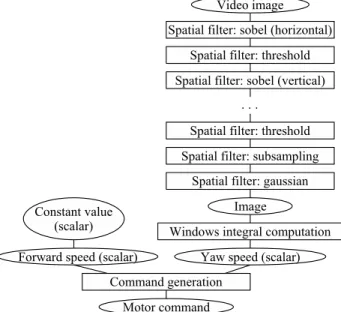
Fig. 1 shows an example controller built with this struc-ture. Rectangles represent primitives and ellipses represent data. The algorithm is a single tree, and all the primitives between the input data and the resulting motor command are created and parameterized by the evolution.
2.2. Environment and Evaluation Function
The environment used for the experiments presented in this paper is a corridor in our lab, i.e. the long central cor-ridor represented on Fig. 2. It’s a relatively simple environ-ment for vision because the floor is dark and the walls are light colored, but the changes in lighting and the openings in the walls create non-trivial challenges for a vision system. The robot that will move in this environment is a Pioneer 3 DX equipped with an onboard PC and a Canon VC-C50i camera. We use 8-bits gray-value images of size320 × 240 representing a field of view of approximately42◦× 32◦, the
Figure 1. Example of a controller for obstacle avoidance based on optical flow.
We want the robot to learn to avoid the walls, in order to be able to wander autonomously in this corridor. For this, we first record several short sequences where we manually guide the robot to move away from the walls and to center itself in the corridor. We record the camera images and the commands given to the robot at each time step. The goal is to find the algorithm that best matches the recorded com-mands given the recorded images. This set of sequences will be our learning base, and we use genetic programming as an offline supervised learning system. Fig. 2 shows some of the trajectories and images we used in this learning base. Note that as we don’t have an absolute positioning system, all the trajectories in this paper are drawn by hand from the video sequences and are thus quite imprecise. In the im-ages, the arrow represents the yaw speed command (maxi-mum left corresponds to30◦/s, maximum right to −30◦/s).
Figure 2. Top: Examples of trajectories used for the learning base. Bottom: Examples of recorded images and commands.
For the evaluation of the algorithms, we replay the recorded sequence offline and compare at each time step the command issued by the evaluated algorithm with the com-mand recorded during the manual control of the robot. The goal is to minimize the difference between these two com-mands along the recorded sequence. Formally, we try to minimize two variablesF and Y defined by the formulas:
F = v u u t n X i=1 (fRi− fAi) 2 andY = v u u t n X i=1 (yRi− yAi) 2
wherefRiandyRiare the recorded forward and yaw speed
commands for frame i, fAi and yAi are the forward and
yaw speed commands from the tested algorithm for framei andn is the number of frames in the video sequence. The evaluations consist in fact in twenty short sequences. Final scores are the means of the scores obtained for the different sequences. Note that as we generally drive the robot at the maximum speed (which is 30 cm/s in these experiments), the forward command is trivial to learn. We’ll focus more on the yaw command for the discussion of the results.
2.3. The Genetic Programming System
We use genetic programming to evolve vision algorithms with little a priori on their structure. As usual with evo-lutionary algorithms, the population is initially filled with randomly generated individuals. We use the grammar based genetic programming system introduced by Whigham [15] to overcome the data typing problem. It also allows us to bias the search toward more promising primitives and to control the growth of the algorithmic tree.
In the same way that a grammar can be used to generate syntactically correct random sentences, a genetic program-ming grammar is used to generate valid algorithms. The grammar defines the primitives and data (the bricks of the algorithm) and the rules that describe how to combine them. The generation process consists in successively transform-ing each non-terminal node of the tree with one of the rules. This grammar is used for the initial generation of the algo-rithms and for the transformation operators. The crossover consists in swapping two subtrees issuing from identical non-terminal nodes in two different individuals. The mu-tation consists in replacing a subtree by a newly generated one. Table 1 presents the exhaustive grammar that we used in these experiments for the creation and transformation of the algorithms.
The numbers in brackets are the probability of selection for each rule. A major advantage of this system is that we can bias the search toward the usage of more promis-ing primitives by settpromis-ing a high probability for the rules that generate them. We can also control the size of the tree by setting small probabilities for the rules that are
Table 1. The genetic programming grammar.
[1.0]START→COMMAND
[1.0]COMMAND→ directMove(REAL,REAL)
[0.2]REAL→ scalarConstant
[0.05]REAL→ add(REAL,REAL)
[0.05]REAL→ subtract(REAL,REAL)
[0.05]REAL→ multiply(REAL,REAL)
[0.05]REAL→ divide(REAL,REAL)
[0.05]REAL→ temporalRegularization(REAL)
[0.05]REAL→ ifThenElse(REAL,REAL,REAL,REAL)
[0.5]REAL→ windowsIntegralComputation(IMAGE)
[0.3]IMAGE→ videoImage
[0.4]IMAGE→SPATIAL FILTER(IMAGE) [0.15]IMAGE→PROJECTION(OPTICAL FLOW)
[0.15]IMAGE→TEMPORAL FILTER(IMAGE)
[0.15]SPATIAL FILTER→ gaussian [0.14]SPATIAL FILTER→ laplacian
[0.14]SPATIAL FILTER→ threshold
[0.14]SPATIAL FILTER→ gabor
[0.14]SPATIAL FILTER→ differenceOfGaussians
[0.14]SPATIAL FILTER→ sobel
[0.15]SPATIAL FILTER→ subsampling
[0.2]TEMPORAL FILTER→ temporalMinimum
[0.2]TEMPORAL FILTER→ temporalMaximum [0.2]TEMPORAL FILTER→ temporalSum
[0.2]TEMPORAL FILTER→ temporalDifference
[0.2]TEMPORAL FILTER→ recursiveMean [0.33]OPTICAL FLOW→ hornSchunck(IMAGE)
[0.33]OPTICAL FLOW→ lucasKanade(IMAGE)
[0.34]OPTICAL FLOW→ blockMatching(IMAGE) [0.2]PROJECTION→ horizontalProjection
[0.2]PROJECTION→ verticalProjection
[0.2]PROJECTION→ euclideanNorm
[0.2]PROJECTION→ manhattanNorm
[0.2]PROJECTION→ timeToContact
likely to cause an exponential growth (rules like REAL →
ifThenElse(REAL,REAL,REAL,REAL) for instance). The parameters of the primitives are generated randomly when the corresponding rule is selected. We define the bounds for each parameter along with the distribution to use for its generation (uniform or normal). For normal distribution we also define the mean value of the parameter and its standard deviation.
As described previously, we wish to minimize two cri-teria (F and Y ). For that, our system uses the widely used multi-objective evolutionary algorithm called NSGA-II in-troduced by K. Deb [5]. Nevertheless, the forward speed command is trivial to learn in this experiment so a classi-cal mono-objective evolutionary algorithm would probably have given similar results.
In order to prevent premature convergence, we separate the population of algorithms in 4 islands, each containing 100 individuals. Those islands are connected with a ring topology; every 10 generations, 5 individuals selected with
binary tournament will migrate to the neighbor island while 5 other individuals are received from the other neighbor is-land. The evolution lasts for 100 generations. For the pa-rameters of the evolution, we use a crossover rate of 0.8 and a probability of mutation of 0.01 for each non-terminal node. We use a classical binary tournament selection in all our experiments. Those parameters were determined em-pirically with a few tests using different values. Due to the length of the experiments, we didn’t proceed to a thorough statistical analysis of the influence of those parameters.
3. Experiments and Results
3.1. Analysis of the Evolved Controllers
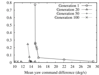
In total, the learning phase lasts for 100 generations, that is 40,000 evaluations. Fig. 3 presents the Pareto fronts ob-tained by taking the best algorithms in all the four islands at different times of the evolution and keeping only non-dominated ones. As said before, the target forward com-mand is almost constant in all the learning set so it is very easy to learn. For the yaw command, we clearly see a pro-gressive improvement from the first generation to the last.
0 0.1 0.2 0.3 0.4 0.5 0.6 0.7 0.8 10 12 14 16 18 20 22 24 26 28 30
Mean forward command difference (m/s)
Mean yaw command difference (deg/s) Generation 1 Generation 20 Generation 50 Generation 100
Figure 3. Pareto fronts of the solutions ob-tained along the generations.
We present on Fig. 4 an example of an evolved algo-rithm. Only a part of it can be presented here because the filter chain contains 29 filters. This high number of filters is partly due to bloating, which means that the evolved pro-grams contain some irrelevant parts that have no significant effect on the final result. The only action we took against bloating is to limit the computation time of the algorithm, but it does not prevent the accumulation of quickly com-puted filters like in this case. Several solutions have been proposed to limit bloating in genetic programming. Among them, the inclusion of program size as an independent cri-terion in a multi-objective evolutionary algorithm has been
shown to produce efficient and small-sized programs (see [4] for instance). As we already use multi-objective opti-mization in our system, we plan to adapt and test this tech-nique in the near future.
The second and more interesting reason for this high number is that the evolution found a way to go past a lim-itation of our system. Indeed, the only available operator to transform an image into a scalar is the windows inte-gral computation described before. This operator is well-adapted for the computation of large features in the image, but not for point or edge features. The evolved algorithm uses a sobel filter that produces an edge corresponding to the separation between the wall and the floor. Most of the subsequent filters just enlarge this edge to allow the win-dows integral computation to produce a value depending on this edge. Of course, this could have been done more easily with a simple dilatation filter and we plan to add morpho-logical filters in our system, but the fact that the evolution found a way to go past this limitation is a good indication of the adaptability of this system.
Figure 4. Example of an evolved algorithm. Fig. 5 illustrates the method used by this evolved algo-rithm to compute the motor command. The red arrow is the command issued by the algorithm, the yellow one is the recorded command. The filter chain highlights and enlarges the boundary between the floor and the wall, as well as the more contrasted zone at the end of the corridor. In the re-sulting image, the wall appears completely white and the boundary is darker. This difference is used by the windows integral computation operator to produce a command that drives the robot away from the wall (the resulting command depends on the difference between the mean pixel value of each red window).
Figure 5. Left: Resulting command from the evolved algorithm on an image from the learn-ing base. Right: The same image trans-formed by the filter chain.
3.2. Generalization Performance
In order to test the robustness and generalization perfor-mance of these evolved controllers, we place the robot at different positions in the corridor and let it move driven by the evolved algorithm. The robot should move to the end of the corridor without hitting the walls. We place the robot so that the direction it faces and the corridor make an angle of approximately30◦. This way, the problem is possible to
solve without being trivial. We made about ten tests with different starting positions. Each time, the robot managed to reach the end of the corridor except once where it turned into one of the openings in the wall. In one test, it even turned at the end of the corridor to go into the smaller corri-dor on the right of the map. Fig. 6 shows an example trajec-tory followed by the robot driven by the evolved algorithm presented before. Note that the two last images correspond to situations that were not included in the learning set.
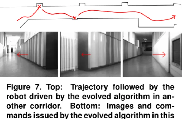
Figure 6. Top: Trajectory followed by the robot when driven by an evolved algorithm. Bottom: Images and commands issued by the algorithm in the generalization tests. We also tested this evolved algorithm in another corridor visually different from the previous one. In one direction the robot reaches the end of the corridor without problem. On the return trip it failed against two obstacles as shown on Fig. 7. The middle and right images correspond to the two obstacles that the robot failed to avoid. Nevertheless
this result is encouraging since this corridor is very different from the one in which the learning base was recorded.
Figure 7. Top: Trajectory followed by the robot driven by the evolved algorithm in an-other corridor. Bottom: Images and com-mands issued by the evolved algorithm in this other corridor.
These experiments prove that our system can produce vi-sion algorithms adapted to a given context to drive a mobile robot in an indoor environment. We now plan to validate it on a wider range of environments. It will also be necessary to give a functional goal to the controllers, like going to a given point or simply exploring the environment as quickly as possible. We have already shown in simulation how to deal with two possibly conflicting goals [2] but we still have to validate these techniques in a real environment.
In real applications, it’s inconceivable to evolve con-trollers for each kind of environment and task the robot may have to face. Our goal is to build a small database of quite generic controllers, to automatically select one depending on the visual context and to adapt it online to improve its performance. We can not use the complete evolution pro-cess online but we could slightly change only the values of the numerical parameters of the algorithm and reward the customized version that drive the robot for the longest time without hitting obstacles for instance. Of course, this would also require a collision detector and a way to move the robot away from the obstacle automatically after the col-lision. But we hope that starting with an evolved algorithm, this adaptation phase could quickly produce efficient algo-rithms and thus make the controllers more adaptable to dif-ferent environments.
4. Conclusion
We presented in this paper a method to automatically generate algorithms adapted to a given environment. We applied it to the obstacle avoidance problem in a real indoor environment. We showed that our system created efficient algorithms, able to drive the robot in a corridor without hit-ting the wall and using only monocular vision. We now plan to design an online system to adapt the vision algorithm de-pending on the context in real-time, in order to have a fully autonomous and adaptive robot.
References
[1] R. Barate and A. Manzanera. Evolving Vision Controllers with a Two-Phase Genetic Programming System Using Im-itation. In From Animals to Animats 10, Proceedings of SAB’08 Conference, pages 73–82, 2008.
[2] R. Barate and A. Manzanera. Generalization Performance of Vision Based Controllers for Mobile Robots Evolved with Genetic Programming. In Proceedings of GECCO
Confer-ence, 2008. To appear.
[3] J. Barron, D. Fleet, and S. Beauchemin. Performance of optical flow techniques. International Journal of Computer Vision, 12(1):43–77, 1994.
[4] S. Bleuler, M. Brack, L. Thiele, and E. Zitzler. Multiobjec-tive Genetic Programming: Reducing Bloat Using SPEA2. In Proceedings of the 2001 Congress on Evolutionary Com-putation, volume 1, pages 536–543, 2001.
[5] K. Deb, A. Pratap, S. Agarwal, and T. Meyarivan. A fast and elitist multiobjective genetic algorithm: NSGA-II. IEEE Transactions on Evolutionary Computation, 6(2):182–197, 2002.
[6] D. Marocco and D. Floreano. Active vision and feature se-lection in evolutionary behavioral systems. In From Animals to Animats 7, Proceedings of SAB’02 Conference, pages 247–255, 2002.
[7] M. Martin. Evolving visual sonar: Depth from monocu-lar images. Pattern Recognition Letters, 27(11):1174–1180, 2006.
[8] J. Michels, A. Saxena, and A. Ng. High speed obstacle avoidance using monocular vision and reinforcement learn-ing. In Proceedings of the 22nd international conference on Machine learning, pages 593–600, 2005.
[9] L. Muratet, S. Doncieux, Y. Bri`ere, and J.-A. Meyer. A contribution to vision-based autonomous helicopter flight in
urban environments. Robotics and Autonomous Systems,
50(4):195–209, 2005.
[10] O. Pauplin, J. Louchet, E. Lutton, and A. De La Fortelle. Evolutionary Optimisation for Obstacle Detection and
Avoidance in Mobile Robotics. Journal of Advanced
Computational Intelligence and Intelligent Informatics, 9(6):622–629, 2005.
[11] A. Saxena, S. Chung, and A. Ng. 3-D Depth Reconstruction from a Single Still Image. International Journal of Com-puter Vision, 76(1):53–69, 2008.
[12] L. Trujillo and G. Olague. Synthesis of interest point
de-tectors through genetic programming. In Proceedings of
GECCO Conference, pages 887–894, 2006.
[13] I. Ulrich and I. Nourbakhsh. Appearance-based obstacle de-tection with monocular color vision. In Proceedings of AAAI Conference, pages 866–871, 2000.
[14] J. Walker, S. Garrett, and M. Wilson. Evolving controllers for real robots: A survey of the literature. Adaptive
Behav-ior, 11(3):179–203, 2003.
[15] P. Whigham. Grammatically-based genetic programming. In Proceedings of the Workshop on Genetic Programming: From Theory to Real-World Applications, pages 33–41, 1995.