HAL Id: hal-01462352
https://hal.archives-ouvertes.fr/hal-01462352
Submitted on 6 Jun 2020
HAL is a multi-disciplinary open access
archive for the deposit and dissemination of sci-entific research documents, whether they are pub-lished or not. The documents may come from teaching and research institutions in France or
L’archive ouverte pluridisciplinaire HAL, est destinée au dépôt et à la diffusion de documents scientifiques de niveau recherche, publiés ou non, émanant des établissements d’enseignement et de recherche français ou étrangers, des laboratoires
a simulation analysis
Daniel Thiel, Vincent Hovelaque, Thi Le Hoa Vo
To cite this version:
Daniel Thiel, Vincent Hovelaque, Thi Le Hoa Vo. Impact of inventory inaccuracy on service level quality: a simulation analysis. [University works] auto-saisine. 2009, 26 p. �hal-01462352�
Impact of inventory inaccuracy on service-level quality:
A simulation analysis
Daniel THIEL, Vincent HOVELAQUE, Thi Le Hoa VO
Working Paper SMART – LERECO N°09-01
January 2009
Impact of inventory inaccuracy on service-level quality:
A simulation analysis
Daniel THIEL
LEM, University of Nantes, France ENITIA, Nantes, France
Vincent HOVELAQUE
Agrocampus Ouest, UMR1302, F-35000 Rennes, France INRA, UMR1302, F-35000 Rennes, France
Thi Le Hoa, VO
LEM, University of Nantes, France
Auteur pour la correspondance / Corresponding author Vincent HOVELAQUE
UMR SMART – Agrocampus Ouest 65 rue de Saint-Brieuc, CS 84215 35042 Rennes cedex, France
Email: [email protected] Téléphone / Phone: +33 (0)2 23 48 54 19
Impact of inventory inaccuracy on service-level quality: A simulation analysis
Abstract
This article discusses the impact of inventory inaccuracy on service-level quality in (Q,R) continuous review, lost-sales inventory models. A simulation model is built to study the behavior of this kind of model exposed to an inaccuracy in inventory records as well as demand variability. We have observed an unusual result which goes against certain empirical practices in the SMEs that consist in hiking the inventory level proportionally to the data inaccuracy rate. A non-monotone function shows that at the outset, the service-level quality is lowered as the inaccuracy rate increases but when the inaccuracy rate becomes much higher this quality is conversely enhanced. This relation can equally be observed given that stocktaking commences as soon as the threshold of decline in the service-level rate has been reached and when demand consequently dwindles. Finally, another noteworthy result also shows the same phenomenon between the function involving a level of safety stock defined by the simulation and the function between the service-level quality and the inventory inaccuracy. These different observed results are discussed in terms of both contribution to the (Q,R) inventory management policies in SMEs and of the limitations to this study.
Keywords: Continuous review inventory system, inventory inaccuracy, continuous model,
discrete-time simulation
Impact des erreurs de stock sur la qualité de service : Une analyse par la simulation
Résumé
Cet article s’intéresse à l'impact de l'erreur d'inventaire sur le taux de qualité de service par le développement et l’analyse d’un modèle de simulation. Ainsi, il est observé un résultat inhabituel qui va à l'encontre de certaines pratiques empiriques dans les PME, qui positionnent le niveau d'inventaire au prorata du taux d'inexactitude des données. Une fonction non-monotone montre que la qualité de service peut augmenter quand le taux d'erreur devient très important. Un autre résultat montre également le même phénomène avec la fonction du niveau de stock de sécurité défini par simulation. Ces différents résultats observés sont discutés en termes de contribution à la théorie liée aux politiques de commande pour les modèles de gestion de stock de type (Q, R).
Mots-clefs : Gestion des stocks, erreur d’inventaire, simulation discrète
Impact of inventory inaccuracy on service-level quality: A simulation analysis
1. Introduction
Inventory record inaccuracy, the discrepancy between the recorded inventory quantity and the actual inventory quantity physically present on the shelf, is a recurring occurrence of often considerable proportions, particularly in the small and medium enterprises (SMEs) (see a literature review proposed by Schrady, 1970). Various observations have recorded the inventory inaccuracy rates amounting to more than 50%. For example, DeHoratius and Raman (2008) examine nearly 370,000 inventory records from 37 stores of one retailer in the USA and find 65% to be inaccurate. According to the authors, the existence of inventory inaccuracy is due to replenishment errors, employee pilfering, shoplifting, improper handling of damaged merchandise, imperfect inventory audits, and incorrect recording of sales. In addition, Kök and Shang (2004) show that the percentage of inventory records that were inaccurate totaled 1.6% of the total inventory value ($10 million worth of inventory) of the Beta enterprise in 2004. The authors justify such divergences between inventory records and physical inventory with stock loss, transaction errors, and misplaced products, all very difficult to rectify, particularly in SMEs. They also state that the direct effect of inventory record inaccuracy is losses resulting from an ineffective inventory order decision. In fact, Iglehart and Morey (1972) already supposed that such divergences may be introduced due to time lags between flows of information and material, pilferage, incorrect units of issue, inaccurate physical inventory counts, etc. For them, the primary impact of these inaccuracies is that the system fails to order when it should, resulting in so-called “warehouse denials”.
As an example, let us consider a biscuit manufacturer that often sends from warehouse to factory the raw materials for which the quantity can correspond to a consumption that is ten-times bigger than the real customer orders or production lots (full sacks of flour, big barrels or sacks, etc.). Therefore, the inventory level is inaccurate because each related lot reduces the flour inventory level with a quantity that does not correspond to the real quantity shipped from the warehouse to the factory. These food companies rarely have a computer-controlled manufacturing process, so the ingredients cannot be measured in real time. In addition, reducing the volume of the bags or
setting up the precise quantity for each lot would increase the handling costs and any automation of such operations would require a high investment that often cannot be financially borne by SMEs.
Nowadays, in order to address the economic consequences of the inventory inaccuracy, the experts propose an improvement in data quality for inventory management technologies based on advanced information such as the Radio Frequency Identification (RFID). In the SMEs, certain business process improvements might be achieved with RFID technology such as cutting inventory costs, labor costs, stock losses when filling more orders, branding and consumer information, etc. Active and semi-passive RFID tags are useful for tracking high-value goods that need to be scanned over long ranges, but are still too expensive to put on low value items such as food products. Most companies limit the tags on the product packages which limit inaccuracy in warehouses but not, for example, for the unit product on the store shelves. Additionally, even with the advanced information systems of regular inventory, the intensity of computerization in various SMEs is still insufficient. What is more, these SMEs have neither the availability of a sufficient workforce and budget to enhance performance nor the capacity to invest in such kind of equipment. In case of inaccuracy in measuring inventory levels, stock management is carried out on the basis of incorrect data resulting in a shortage issue. Hence, simultaneously facing this inventory inaccuracy problem and a plethora of uncertainties, SMEs usually react by estimating an empirical level of safety stock.
From a theoretical point of view, many papers consider such problems with inventory policy approaches and/or management of information in various and numerous assumptions. Some researchers lay emphasis on optimizing the counting or information systems, or on the required buffer size to minimize shortage risk and costs. To our knowledge, the works on optimizing safety stock (e.g. Shin, 1999; Ross, 2002; Atali et al., 2005; Tan et al., 2007) never take into consideration the risk induced by inventory inaccuracy.
Most researchers do indeed introduce the fluctuation of demand and shipment delay, but few of them take inventory inaccuracy into account. Their research usually focuses on (Q,R) system optimization models under uncertainties in lead-times, demand, supply, machine breakdown, etc., but it rarely appraises the effect of inventory inaccuracy upon service-level quality. For example, Sahin et al. (2008) propose a newsvendor type model which analytically derives the optimal
policy in the presence of records errors of evenly distributed inventory and demand in the supply chain. Rekik et al. (2008) have also developed an analytical model of a single-period store inventory model subject to misplacement errors and compare it to a RFID implemented inventory system. Another analysis focuses on the inventory inaccuracy reduction aspect of RFID technology and on the problem of finding the optimal investment levels that maximize profit by decreasing inventory inaccuracy (Uçkun et al., 2008).
Therefore, we recognize that the impact of inventory inaccuracy on service quality in (Q,R) continuous review, lost-sales inventory models has not attained the acceptable levels as of yet. Such is the reason why we attempt to study such an important issue in this paper.
Firstly, we introduce a literature review in order to show that there exists little research which deals with the impact of inventory inaccuracy on service-level quality subjected to demand fluctuations. Secondly, we describe the simulation model based on a (Q,R) policy taking into account inaccuracies in inventory records. Thirdly, we discuss the simulation results showing a non-monotone function between the quality of service and the inventory inaccuracy rate. The fourth section involves our analysis of the influence of inventory counting as well as demand degradation in the case of poor quality of service. Finally, we conclude our study by showing that the results could contribute to the process of determining a new safety stock policy relating to inaccuracy in inventory records.
2. Literature review
Research on inventory record inaccuracy has been taking place since the 1960s with the report by Rinehart (1960) on a case study of a Federal government supply facility. The author stated that this inaccuracy produces a “deleterious effect” on operational performance. Following this, Iglehart and Morey (1972) reported that this divergence between stock record and physical stock results in “warehouse denials”. Their research took into consideration the frequency and depth of inventory counts and stocking policy to minimize total cost per time unit. Studying a similar problem, Kök and Shang (2004) have suggested implementing a cycle count program and carefully adjusting base-stock levels across periods to minimize total inventory and inspection costs. Moreover, focusing on the significance of measuring inventory record inaccuracy, DeHoratius and Raman (2008) show that inventory counts may not impact record inaccuracy and
additional buffer stock may not be equally necessary across all items in all stores. They also suggest that inventory density and product variety have substantial implications for identifying and eliminating the source of inventory record inaccuracy. However, their study is only based on the retail stores of one firm and does not include all factors that might impact variation in inventory record inaccuracy from one store to the next.
In fact, safety stock in the continuous-review lost-sales inventory models is one of the effective inventory management policies for mitigating long run total cost. Ritchken and Sankar (1984) used a regression-based method to adjust the size of the stock by incorporating an additional safety stock requirement in order to estimate the risk in inventory problems. Persona et al. (2007) have suggested that by introducing a safety stock of pre-assembled modules or components, one can reduce the occurrence of stock-outs. On considering the continuous-review lost-sales inventory models with Poisson demand, Hill (2007) shows that a base stock policy is “economically” optimal, and that computing the optimal base stock and its corresponding cost is quite simple for a backorder model. However, for a lost-sales model, this policy is not optimal but the size of the state space means that determining the optimal policy is unfeasible. Hence, the author proposes three alternative policies. Two of these involve modifying the optimal base stock policy by imposing a delay between the placements of successive orders. The third policy is to place orders at pre-determined fixed and regular intervals. However, these policies require a lot of complex calculations for lead times under demand uncertainty.
Moreover, among the few works appraising record inaccuracy in inventory management policies, the research by Kang and Gershwin (2004) is the most closely related to our research. The authors use analytical and simulation modeling to investigate the problems caused by information inaccuracy in inventory systems. By applying the (Q,R) policy, they suggest that a small rate of stock loss can disrupt the replenishment process and create severe shortages of stock. Their simulation obtains 1% and 2.4% inventory inaccuracy in out-of-stock levels at 17% and 50% respectively. Their results also reveal that the harmful effect of stock loss is greater in lean environments with short lead times as well as with small amounts of orders. According to these authors, the inventory inaccuracy problem can be effectively controlled if the stochastic behavior of the stock loss is known. In addition, Kumar and Arora (1992) have already applied quantitative measures and find that the quality of service-level declines in a continuous review (Q,R) inventory policy when there are inventory miscounts and variations in lead time.
Even though most of the current research focusing on (Q,R) policy often proposes models of operational research, simulation modeling is becoming an effective and timely tool and is capturing the cause and effect relationship in this field (e.g. the previously mentioned research by Kang and Gershwin (2004)). Moreover, Fleisch and Tellkamp (2005) use simulation and variance analysis to study the individual impacts of different types of inaccuracies on the performance measurements of cost, system inventory inaccuracy and out-of-stock percentages of a three-echelon supply chain.
In summary, among all these papers which tackle record inaccuracy in inventory management policies, there is only one published paper primarily studying the impact of inaccurate inventory on quality of service (Fleisch and Tellkamp, 2005). Albeit so, the relationship between the inventory inaccuracy and the service-level quality, as well as the stock-out opinion were not considered in this study. Therefore, in this paper we will attempt to extend the previous research and fill this gap in the literature by exploring the impact of inventory inaccuracy on service-level quality under the variation of demand and different inventory management policies.
3. Model description
We will now describe the structure of a simulation model taking into account inventory record inaccuracy. Beforehand, let us refer to the principles and the objectives of the (Q,R) models.
The (Q,R) policy is a generalization of the EOQ model in which the inventory is managed by a fixed order quantity Q and a fixed reorder level R subject to an uncertain demand (Nahmias, 2001). The demand is a continuous random variable with probability density function f(δ) and cumulative distribution function F(δ). The optimal policy is defined by the minimization of the total cost function G(Q,R):
∫
∞ − = + + − + = R d f R R n R n Q p Q k L R Q h R Q G µ ) µ µ ( ) with ( ) (δ ) (δ) δ 2 ( ) , (where h, k and p are respectively holding, ordering and shortage costs. L is the order lead time and µ the expected unit time average demand. The optimal solution is obtained by solving the two equations:
µ µ p hQ R F h R pn k Q= 2 ( + ( )) and 1− ( )=
In reality, SMEs have difficulties in approximating the different costs h, k and p. Moreover, the stock-out cost is complex to evaluate because it includes intangible parameters such as loss of branding, referencing, etc. As a result, most enterprises drive their inventory with empirical policies. In accordance with this established fact, we propose a (Q,R) model described below.
Let us consider a warehouse which holds stock and a retailer who follows a continuous review (Q, R) policy. Following Kang and Gershwin (2004), we consider that the inventory records X1,
X2,… suffer from inaccuracy information which would lead to shortages. For each period k, the
demand δk is assumed to be independent and normally distributed with mean µ and standard
deviationσd. At the beginning of a period k, the real inventory level is equal to Xk. If a supply is
delivered during this period k, the on-hand stock is Xk+Q. Thus, the demand δk is compared either
to Xk or to (δk + Q) depending on an order placed at period k-L with L = shipment time. The
inventory evolution can be described by the following relationship:
{
,0}
min 1 k k k k X Q S X + = + × −δ with − = otherwise 0 at placed order was an if 1 k L SkThe manufacturer faces shortage if: δk >(Xk +Q×Sk).
We have now to include the supply decision process. We make the assumption that the manager has an approximate knowledge of the stock levelX . A supply order is placed if the on-hand k
estimated stock Xk
~
is less than R and if there is no inventory on-order (that is, there is no supply delivered between k and k+L). Then the supply order process is defined as follows:
= < =
∑
− − = − otherwise 0 0 and ~ if 1 1 k L k j j L k k S R X SFinally, this model is based on two inventory level comparisons: demand and the real inventory levels, and the approximate inventory with the reorder point levels.
The objective of this paper is not to define an optimal policy for inventory management but to analyze the service-level evolution under different model parameters.
In this lost-sales case, the service-level is defined by cumulating the number of inventory shortages and the total quantity of loss-sales during a definite period of time (there is no order backlog). To consider an inaccuracy in the inventory level, we define εk as an error of inventory
estimation at each period k. Inventory inaccuracy is a continuous random variable which is independently and identically distributed with mean 0 and standard deviationσε . Thus, the sequence at each period is assumed to be as follows:
• The real component inventory of X is adjusted: Xk + SkQ (with Sk defined previously).
• The demand is revealed by δk. The demand is totally satisfied (if Xk+SkQ < δk or not
(loss-sales of δk -Xk + SkQ).
• The inventory level is approximated by X~k = Xk +εkand a supply order is placed ifXk <R
~
.
This analytical formulation of the problem will now been translated into a continuous model with discrete-time simulation as follows:
Model constants:
Demand: δ = 300 per hour Delivery time: L = 18 hours
Reorder point: R = δ L
Order quantity inventory coverage time: z = 64 hours
Model parameters:
Simulation time: T = 32,000 hours
Time step : dt = 1 hour
Inventory inacuracy standard deviation σε = 150 Model equations:
Xt =
∫
T 0 dt . ) X' -.z (δ X0 = δ . z If Xt < δ then Xt’= Xt else Xt’ = δInaccurate inventory record X~t = Xt + N (0 ,σε)
Q order launching
When order launching then: Q’ = Q after L = 18 hours delivery time
IF Q’ > 0 then Q = 0 else IF ( X~t < R) then Q = δ.z else Q = 0
Number of products out-of-stock during time T = 32,000 hours
Krt =
∫
Θ T 0 dt . Kr0 = 0 If Xt = 0 then Θ = 1 else 0This model has been simulated using Euler integration and for each inventory imprecision rate the simulation was run 100 times, with different seeds and during a run-in period of 1,000 hours followed by a recording period of T = 32,000 hours. The simulations were also tested with different values of Q and R. Because we observed that these variables bear no influence on the simulation main results, we finally do not include cost parameters in our model.
For each running time, the service-level quality is evaluated by recording the value of Krt
according to each value of the inventory inaccuracy rate defined by: IR = σε/ R.
4. Impact of the inventory record inaccuracy on the quality of service
Figure 1 shows a non-monotone relationship between the number of shortages Kr cumulated after
a total simulation time of 32,000 hours and the inventory inaccuracy rate IR. A peak is observed for the values of IR featured from 5 % to 15%; and there is a decrease in Kr when IR increases
more. As we can see in Figure 1, when the IR is below 12%, an increase in IR will speedily increase the number of shortages Kr, but it drops sharply as the IR continues to increase until the
IR attains 20%. After that, the number of shortages Kr decreases slightly while the IR continues to
progress.
Figure 1: Variation of Kr with IR (constant demand)
0 2000 4000 6000 8000 10000 12000 14000 16000 0% 10% 20% 30% 40% 50% 60% 70%
IR : Inventory inaccuracy rate
K r : N u m b er o f sh o rt a g es d u ri n g 3 2 0 0 0 h o u rs
The curve on Figure 1 was observed using a constant demand. In the case of a Normal distributed demand, we consider that SMEs’ deciders choose to empirically increase the reorder point level R according to the demand fluctuations to avoid shortages whenσε is high. Taking this hypothesis, we observe the same peak in Kr = f( IR).
We will now try to analytically explain the reason for such phenomena showing no monotony of the service-level quality according to the inventory inaccuracy rate.
First of all, it is necessary to describe the inventory evolution over time in order to explain this peak. Thus, we assume that the system does not encounter any shortages until instant i, the inventory equations at the beginning of the period i being described as follows:
1 1 0 1 1 1 − − − − − Π + ∆ − = × + − = i i i i i i X S Q X X δ where :
∑
− = − = ∆ 1 1 1 i j ji δ (cumulative demands during [1, i-1]), and
∑
− = − = × Π 1 1 1 i j j i Q S
(replenishments lumping during [1, i-1]).
Therefore, we can consider that there is enough inventory input to ensure no shortages during the period of [1, i-1], which means that: M =X0 +Πi−1 ≥∆i−1
Moreover, the demand follows a Normal distribution(µ,σd), independently over time with different random values withδj. Thus, the cumulated demand during the period of [1, j], with
1
2≤ j≤i− follows a Normal distribution((j−1)µ, j−1σd).
Secondly the estimated stock level at the beginning of the period i is defined as: Xi = Xi +εj
~
,
with εj following a Normal distribution (0,σε). In this case, with a hypothesis of no shortage
during [1, i], the estimated stockX~j follows a Normal distribution ((j−1)µ, (j−1)σd2 +σε2) with 2≤ j≤i−1.
We will now study the case where the estimated level of stock at time i is higher than the reorder point R while the real level of stock is lower than R. According to the simulation result, this phenomenon will generate a risk of shortage throughout the period of [i, i+l], with L = shipment time. Therefore, this shortage risk is recorded by following three conditions:
1 and one least at for 1 1 and all for ~ − + ≤ ≤ < − ≤ ≤ > < − L i k i k X i j j R X R X k k j i i δ
Using the above descriptions of random variables Xj Xj
~
et and on condition that these variables are associated with the statistic laws, we obtain:
1 and one least at for 1 ) Pr( 1 1 and all for ) ( ) ( ) ~ Pr( ) 1 ( ) 1 ( 1 ) Pr( 2 2 2 2 − + ≤ ≤ − − = < − ≤ ≤ + − − − − = > − − − − − = < − L i k i k k k M d X i j j j i j i R M R X i i R M R X d k k d j i d i σ µ φ σ σ µ φ σ µ φ ε
with φ(a)=Pr(Z<a) where Z follows a standard normal law.
These combined conditions reveal the possible risk of shortages at time i: a stock overestimation dissimulating a need for carrying a refilling. Mathematically, the associated function is concave withσε, which corroborates the obtained simulation results.
This finding is illustrated in Figure 2 showing the expression ) Pr( ) ~ Pr( ) ~ Pr( ) ~ Pr( )
Pr(Xi <R × Xi−1 >R × Xi−2 >R × Xi−3 >R × Xk <δk in comparison with the
previous simulations results Kr = f( IR) showed in Figure 1.
Figure 2: Comparison between simulation and analytical models
0% 1% 2% 3% 4% 5% 6% 7% 8% 9% 0 3% 6% 10% 14% 19% 28% 37% 46% 70%
Ir : Inventory inaccuracy rate
P r o b a b il it ie s o f sh o r ta g e s 0 2000 4000 6000 8000 10000 12000 14000 16000 K r : N u m b e r o f sh o r ta g e s d u r in g 3 2 ,0 0 0 h o u r s Analytical Model Simulation model
The noteworthy result from this observation is that the shapes of both these curves showed in Figure 2 are almost similar, demonstrating a peak of the non-monotony between the service-level
quality and the inventory inaccuracy. Nevertheless, these two models deal with different indicators. In fact, the analytical model deals with shortage probabilities and the simulation model focuses on cumulative shortages during a fixed time period of simulation.
4.2. Problem extensions
4.2.1. Relationship between safety stock level and inventory inaccuracy
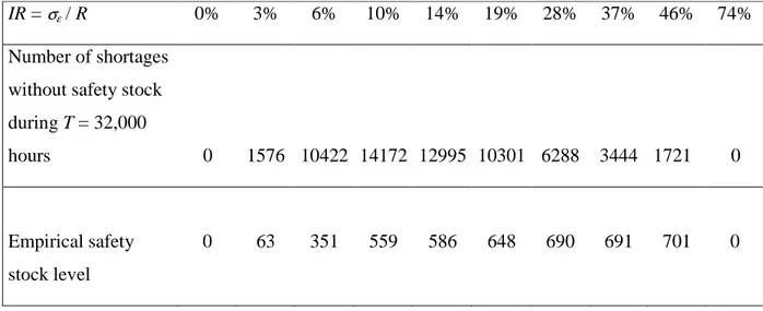
For each inventory inaccuracy rate IR, we simulate 100 times the previous model with constant demand and we define a level of safety stock which avoids any shortages for T = 32,000 hours with a high probability. Once this value is defined, we then add this safety stock value to the value of the reorder point level R and run the model with these new values. Finally, we compare the level of safety stock to the cumulated number of shortages according to the inaccuracy rate IR (see Table 1 and Figure 3).
Table 1: Level of safety stock empirically defined vs. inventory inaccuracy rate IR
IR = σε / R 0% 3% 6% 10% 14% 19% 28% 37% 46% 74%
Number of shortages without safety stock during T = 32,000 hours 0 1576 10422 14172 12995 10301 6288 3444 1721 0 Empirical safety stock level 0 63 351 559 586 648 690 691 701 0
Figure 3: Evolution of safety stock level and service-level quality with inventory inaccuracy rate (with σd = 0 + ) 0 2000 4000 6000 8000 10000 12000 14000 16000 0% 3% 6% 10% 14% 19% 28% 37% 46% 70%
IR : Inventory inaccuracy rate
K r: N u m b e r o f sh o r ta g e s d u r in g 3 2 ,0 0 0 h o u r s 0 100 200 300 400 500 600 700 800 E m p ir ic a l le v e l o f sa fe ty s to c k Number of shortages Safety Stock Level
We can see that the curve of safety stock level vs. inventory inaccuracy rate IR in Figure 3 has a peak which is out of phase with the peak observed in Figure 1 in the curve Kr according to IR.
These results confirm a non-monotone function between the service-level quality as well as a safety stock level and the inventory inaccuracy rate in the simulation model.
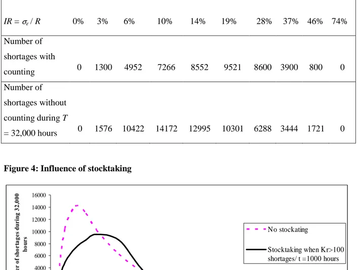
4.2.2. Impact of inventory counting
We now assume that if the number of cumulative shortages is greater than a fixed threshold, the company will decide to launch stocktaking as a way for correcting these inventory measurement errors.
Let us consider that inventory counting begins after 100 consecutive shortages. After stocktaking, the inventory will be readjusted as follows: between time t0 of stocktaking and time (t0+τ) with τ
equal to 1,000 hours, we assume that the inventory inaccuracy rate will increase from 0 to εj
following a sigmoid curve.
Table 2: Influence of stocktaking IR = σε / R 0% 3% 6% 10% 14% 19% 28% 37% 46% 74% Number of shortages with counting 0 1300 4952 7266 8552 9521 8600 3900 800 0 Number of shortages without counting during T = 32,000 hours 0 1576 10422 14172 12995 10301 6288 3444 1721 0
Figure 4: Influence of stocktaking
0 2000 4000 6000 8000 10000 12000 14000 16000 0% 10% 20% 30% 40% 50% 60% 70%
IR : Inventory inaccuracy rate
K r: N u m b e r o f sh o r ta g e s d u r in g 3 2 ,0 0 0 h o u r s No stockating Stocktaking when Kr>100 shortages/ t =1000 hours
Figure 4 compares the case of non stocktaking and the case with inventory counting. It shows that when there is no stocktaking, there is a non-monotone relationship between the number of shortages Kr cumulated and the inventory inaccuracy rate IR as shown in the previous section
with a high shortages peak of 14,172 units for 10% of inventory inaccuracy. On the other hand, when inventory counting is carried out, the number of cumulative shortages Kr is considerably
19%. This confirms that it is possible to use stocktaking to mitigate the quantity of cumulative shortages in the event of inventory inaccuracy.
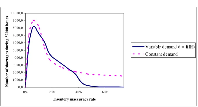
4.2.3. Case of demand rate decreasing when quality of service decreases
We now consider that the demand δ decreases according to the cumulative number of out of stock products. We assume that the demand follows an S-shaped curve corresponding to a slow decrease in the sales when the number of shortage increases and then a quick decrease to finally stabilize demand.
Given a third order exponential function between δ and Kr, the reorder point R is re-calculated
during simulation according to the demand fluctuations without safety stock. For such a scenario, the same peak is observed (see Table 3 and Figure 5) which also confirms our global observations about the type of relationship between the quality of service and the inventory inaccuracy rate.
Table 3: Demand varying according to Kr
IR = σε / R 0% 3% 6% 10% 14% 19% 28% 37% 46% 74%
Number of shortages during T = 32,000 hours
Figure 5: Influence of variable demand δδδδ = f(IR) 0,0 1000,0 2000,0 3000,0 4000,0 5000,0 6000,0 7000,0 8000,0 9000,0 10000,0 0% 20% 40% 60%
Inventory inaccuracy rate
N u m b e r o f sh o r ta g e s d u r in g 3 2 0 0 0 h o u r s
Variable demand d = f(IR) Constant demand
As we can observe in Figure 5, the global shape of K = f(IR) is quite similar but in the case of a demand decrease resulting from high number of stock-outs, the service-level quality only gets perfect when IR > 50%.
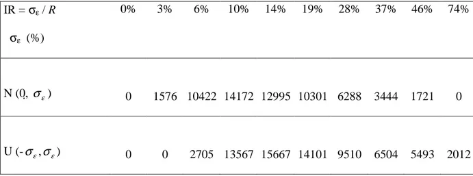
4.2.4. Impact of inventory inaccuracy error distribution function
Finally, we also test our main observations by comparing two inaccuracy rate distribution functions:
- a Normal distribution N(0, σε) with σε = standard deviation and mean 0.
- a Uniform distribution U(-σε,σε) with the following probability density function :
> − < ≤ ≤ = ε ε ε ε ε σ σ σ σ σ x x x x f or for 0 -for 2 1 ) (
Table 4: Inventory inaccuracy rate with Normal and Uniform error distribution IR = σε / R σε (%) 0% 3% 6% 10% 14% 19% 28% 37% 46% 74% N (0, σε) 0 1576 10422 14172 12995 10301 6288 3444 1721 0 U (-σε,σε) 0 0 2705 13567 15667 14101 9510 6504 5493 2012
We can observe in Figure 6 the same phenomenon in both cases with a peak in the case of a Uniform distribution which corresponds to a larger “bell curve” than in the Normal error distribution. This can be explained by the fact that the probability density function of a Uniform function covers a wider area with equiprobability between -σε and σεwhile a Normal function is a bell curve centered on its mean 0.
Figure 6: Influence of error distribution functions
0 2000 4000 6000 8000 10000 12000 14000 16000 18000 0% 10% 20% 30% 40% 50% 60% 70%
IR : Inventory inaccuracy rate
K r: N u m b e r o f sh o r ta g e s d u r in g 3 2 ,0 0 0 h o u r s Normal Distribution N(0,s) Uniform Distribution U(-s,s)
5. Discussions and research outlooks
In the first place, by using simulation this research has shown an original non-monotone function between the service-level quality and the inventory inaccuracy rate. The relationship between these two variables is quite complex. In fact, the service-level initially declines as the inaccuracy rate increases and then it improves at or after a threshold. We have validated this observation even in cases where the stocktaking was performed and demand dropped when the service-level quality declined. We have also analytically studied the problem by trying to demonstrate this surprising phenomenon.
Secondly, our results could be empirically meaningful. In fact, the service-level rate improves given that the inaccuracy rate is considerable. This can be explained by the fact that when σεis high the measured values are found not to be higher than the threshold of replenishment rate R (real risk of shortage) but also below R which in this case, induces an anticipated setting-off of the order Q. The fact that this frequency is strong will cause the shortage risk to diminish.
Even though the results in this study are based on simulation modeling, we have attempted to theoretically justify the observed phenomenon by defining the shortage probabilities in the case that the real stock level is below the replenishment threshold and also the measured inventory exceeds the same threshold. A discrete state, continuous parameter Markov process approach should be equally worth developing by considering a state space representing the product inventory level and the transitions corresponding to the probabilities of consumption and ordering. However, the difficulty in using this method would be in integrating the stochastic characteristic of the measuring inaccuracy of these states into a discrete state space.
Thirdly, we make every effort to study our observations more thoroughly by determining an optimal safety stock level according to the inventory inaccuracy rate. The expression
) Pr( ) ~ Pr( ) ~ Pr( ) ~ Pr( ) Pr(Xi <R × Xi−1 >R × Xi−2 >R × Xi−3 >R × Xk <δk described in Section 4.1
could be derived in order to find the maximum number of shortage probabilities.
In the fourth place, as shown in Figure 3, we would like to further understand the observed gap between an empirically defined safety stock and simulated service quality in terms of an inaccuracy rate. According to the simulation results, the variation of the safety stock level is contrary to that of service-level quality. This confirms the study of Morey (1985) that the
maintenance of additional safety stock is one of the management mechanisms for improving service-level when one is faced with inventory record inaccuracy. Moreover, this research enables a decision-maker to establish a sufficient safety stock if the average inventory inaccuracy rate is found in a given interval. Beyond this interval, no safety stock is necessary for either small or high values of the inventory inaccuracy rate.
Finally, the degradation of the service-level quality due to inventory inaccuracy consequently results in unexpected costs and affects the enterprises’ profit margin or worsens their performance. Accordingly, we will be further using our model to measure the extra costs and marginal profit of inventory inaccuracy effects and studying how the inventory policies offered in this paper could help managers to moderate these costs and improve their performance.
References
Atali, A., Lee, H., Ozer, O. (2005). If the inventory manager knew: Value of RFID under imperfect inventory information. Technical Report, Graduate School of Business, Stanford University.
DeHoratius, N., A. Raman. (2008). Inventory record inaccuracy: an empirical analysis. Management Science, 54(4): 627-641.
Fleisch, E., Tellkamp, C. (2005). Inventory inaccuracy and supply chain performance: a simulation study of a retail supply chain. International Journal of Production Economics, 95(3): 373-385.
Hill, R.M. (2007). Continuous-review, lost-sales inventory models with Poisson demand, a fixed lead time and no fixed order cost. European Journal of Operational Research, 176 (2): 956-963.
Iglehart, D., Morey, R.C. (1972). Inventory systems with imperfect asset information; Management Science, 18(8): 388-394.
Kang, Y., Gershwin, S. B. (2004). Information inaccuracy in inventory systems - stock loss and stock-out. IIE Transactions, 37: 843–859.
Kök, A. G., Shang, K., H. (2004). Replenishment and inspection policies for systems with inventory record inaccuracy. Technical Report, Fuqua School of Business, Duke University.
Kumar, S., Arora, S. (1992). Effects of Inventory miscount and non inclusion of the lead time variability on inventory system performance, IIE Transactions, 24(2): 96-103.
Morey, R. C. (1985). Estimating Service Level Impacts from Changes in Cycle Count, Buffer Stock, or Corrective Action. Journal of Operations Management, 5: 411-418.
Nahmias, S. (2001). Production and operations analysis. 4th edition. McGraw-Hill/Irwin, Boston.
Persona, A., Battini, D., Manzini, R., Pareschi, A. (2007). Optimal safety stock levels of subassemblies and manufacturing components. International Journal of Production Economics, 110(1-2): 147-159.
Rekik, Y., Sahin, E., Dallery, Y. (2008). Analysis of the impact of the RFID technology on reducing product misplacement errors at retail stores. International Journal of Production Economics, 112(1): 264 - 278.
Rinehart, R.F. (1960). Effects and Causes of Discrepancies in Supply Operations.Operations Research. 8(4): 543-564.
Ritchken, P., Sankar, R. (1984). The effect of estimation risk in establishing safety stock levels in an inventory model. Journal of Operational Research Society, 35(12): 1091-1099.
Ross, A. (2002). A multi-dimensional empirical exploration of technology investment, coordination and firm performance. International Journal of Physical Distribution & Logistics Management, 32(7): 591-609.
Sahin E., Buzacott J., Dallery Y. (2008). Analysis of a newsvendor which has errors in inventory data records. European Journal of Operational Research, 188(2): 370-389.
Schrady D.A. (1970). Operational definitions of inventory record accuracy. Naval Research Logistics Quarterly,17 (1): 133-142.
Shin, N. (1999). Does information technology improve coordination? An empirical analysis. Logistics Information Management, 12(1/2): 138-144.
Tan, T., Güllüb, R., Erkip, N. (2007). Modelling imperfect advance demand information and analysis of optimal inventory policies. European Journal of Operational Research, 177(2): 897-923.
Uçkun C., Karaesmen F., Savaş, S. (2008). Investment in improved inventory accuracy in a decentralized supply chain. International Journal of Production Economics, 113(2): 546-566.
Les Working Papers SMART – LERECO sont produits par l’UMR SMART et l’UR LERECO
• UMR SMART
L’Unité Mixte de Recherche (UMR 1302) Structures et Marchés Agricoles, Ressources et Territoires comprend l’unité de recherche d’Economie et Sociologie Rurales de l’INRA de Rennes et le département d’Economie Rurale et Gestion d’Agrocampus Ouest.
Adresse :
UMR SMART - INRA, 4 allée Bobierre, CS 61103, 35011 Rennes cedex
UMR SMART - Agrocampus, 65 rue de Saint Brieuc, CS 84215, 35042 Rennes cedex
http://www.rennes.inra.fr/smart • LERECO
Unité de Recherche Laboratoire d’Etudes et de Recherches en Economie Adresse :
LERECO, INRA, Rue de la Géraudière, BP 71627 44316 Nantes Cedex 03
http://www.nantes.inra.fr/le_centre_inra_angers_nantes/inra_angers_nantes_le_site_de_nantes/les_unites/et udes_et_recherches_economiques_lereco
Liste complète des Working Papers SMART – LERECO :
http://www.rennes.inra.fr/smart/publications/working_papers
The Working Papers SMART – LERECO are produced by UMR SMART and UR LERECO
• UMR SMART
The « Mixed Unit of Research » (UMR1302) Structures and Markets in Agriculture, Resources and Territories, is composed of the research unit of Rural Economics and Sociology of INRA Rennes and of the Department of Rural Economics and Management of Agrocampus Ouest.
Address:
UMR SMART - INRA, 4 allée Bobierre, CS 61103, 35011 Rennes cedex, France
UMR SMART - Agrocampus, 65 rue de Saint Brieuc, CS 84215, 35042 Rennes cedex, France
http://www.rennes.inra.fr/smart_eng/ • LERECO
Research Unit Economic Studies and Research Lab Address:
LERECO, INRA, Rue de la Géraudière, BP 71627 44316 Nantes Cedex 03, France
http://www.nantes.inra.fr/nantes_eng/le_centre_inra_angers_nantes/inra_angers_nantes_le_site_de_nantes/l es_unites/etudes_et_recherches_economiques_lereco
Full list of the Working Papers SMART – LERECO:
http://www.rennes.inra.fr/smart_eng/publications/working_papers
Contact
Working Papers SMART – LERECO INRA, UMR SMART
4 allée Adolphe Bobierre, CS 61103 35011 Rennes cedex, France
2009
Working Papers SMART – LERECO
UMR INRA-Agrocampus Ouest SMART (Structures et Marchés Agricoles, Ressources et Territoires) UR INRA LERECO (Laboratoires d’Etudes et de Recherches Economiques)