Combinatorics related to the totally nonnegative Grassmannian

Combinatorics related to the Totally Nonnegative

Grassmannian

by

SuHo Oh

Submitted to the Department of Mathematics

in partial fulfillment of the requirements for the degree of

Doctor of Applied Mathematics

at the

MASSACHUSETTS INSTITUTE OF TECHNOLOGY

MASSACHUSETTS INSTITUTE OF TECHNOLOGY

SEP 2

2 2011

LiBRARIES

ARCHIVES

September 2011

©

Massachusetts Institute of Technology 2011. All rights reserved.

Author ...

...

Department of Mathematics

June 09, 2011

A

Af~)

.

I

Certified by...

Alexander Postnikov

Associate Professor

Thesis Supervisor

Accepted by ...

Michel Goemans

Chairman, Department Committee on Graduate Theses

Combinatorics related to the Totally Nonnegative

Grassmannian

by

SuHo Oh

Submitted to the Department of Mathematics on June 09, 2011, in partial fulfillment of the

requirements for the degree of Doctor of Applied Mathematics

Abstract

In this thesis we study the combinatorial objects that appear in the study of non-negative part of the Grassmannian. The classical theory of total positivity studies matrices such that all minors are nonnegative. Lustzig extended this theory to arbi-trary reductive groups and flag varieties. Postnikov studied the nonnegative part of the Grassmannian, showed that it has a nice cell decomposition using matroid strata, and introduced several combinatorial objects that encode such cells. In this thesis, we focus on the combinatorial aspects of such associated objects.

In chapter 1, we review the definition of the cells in the totally nonnegative part of the Grassmannian, and the associated combinatorial objects. Each cell corresponds to a certain matroid called positroid. There are numerous combinatorial objects that can represent a positroid, such as a J-diagram, a Grassmann necklace or a decorated permutation. We will go over the definitions of such objects and check some of their properties. And for decorated permutations, there are certain planar graphs called plabic graphs, that plays the role of wiring diagrams for permutations, and this would serve as the main tool for our result in chapter 3.

In chapter 2, we prove a conjecture by Postnikov, that allows us to give a purely combinatorial definition of positroids without relying on its realizability. We will show that positroids can be defined as certain collections that satisfy some cyclic inequalities. In other words, we express positroids using cyclically shifted Schubert matroids. Postnikov showed that each positroid cell is an intersection of the totally nonnegative Grassmannian and cyclically shifted Schubert cells. Combinatorially, this result implies that each positroid is included in an intersection of cyclically shifted Schubert matroids. We extend this result: each positroid is exactly an intersection of certain cyclically shifted Schubert niatroids.

In chapter 3, we study maximal weakly separated collections. Weak separation is a condition on pair of sets that first appeared in Leclerc and Zelevinsky's work describing quasicommuting families of quantum minors. They conjectured that all maximal by inclusion weakly separated collections of minors have the same cardinality (the purity conjecture), and that they can be related to each other by a sequence

of mutations. We link the study of weak separation with the totally nonnegative Grassmannian, by extending the notion of weak separation to positroids. By using plabic graphs, we generalize the results and conjectures of Leclerc and Zelevinsky, and prove them in this more general setup. This part of the thesis is based on joint work with Alexander Postnikov and David Speyer.

In chapter 4, we prove a property on h-vector of positroids. The h-vector of a matroid is an interesting Tutte polynomial evaluation, which is originally defined as the h-vector of the corresponding independent complex of a matroid. Stanley conjectured that h-vector of any matroid is a pure O-sequence, which is a sequence coming froi a Hilbert function of a monomial Artinian level algebra. We show that the conjecture holds for positroids: that is, the h-vector of a positroid is a pure O-sequence.

Thesis Supervisor: Alexander Postnikov Title: Associate Professor

Contents

totally nonnegative Grassmannian

Matroid strata of the Grassmannian . . . . Cells in the totally nonnegative Grassmannian . . . . Le-diagrams and Le-graphs . . . . Plabic graphs . . . . 2 Positroids and Schubert matroids

2.1 Introduction . . . . 2.2 Connections between a J-diagram and a Grassmann necklace

2.3 Proof of the main theorem . . . .

2.4 Decorated pcrmutations and the Upper Grassmann necklace

2.5 Further Remark . . . .

3 Maximal weakly separated collections and Plabic graphs 3.1 Introduction . . . .

3.2 Weakly separated collections . . . . 3.3 Decomposition into connected components . . . .

3.4 Plabic graphs and weakly separated sets . . . .

3.5 Plabic tilings . . . . 3.6 Proof of Lemma 3.6.1 . . . . 3.7 Proof of the Purity Conjecture . . . . 3.8 Connection with w-chamber sets of Leclerc and Zelevinsky

31 . . . . 31 . . . . 33 . . . . 36 . . . . 40 . . . . 44 . . . . 55 . . . . 61 . . . . 65

4 The h-vector of a Positroid is a pure O-sequence. 69

4.1 Introduction . . . . 69

4.2 The h-vector of a positroid is a pure O-sequence. . . . . 70

4.3 Exam ple . . . . 75

Chapter 1

The totally nonnegative

Grassmannian

This chapter focuses on introducing basic terminology and essential tools in [9] that we will be using throughout the thesis. We start out with how a positroid comes from the stratification of the totally nonnegative Grassmannian. Then we look at the combinatorial objects that are in bijection with positroids: Grassmann necklaces, decorated permutations and J-diagrams. We also review plabic graphs, which are planar bicolored graphs that encodes various information of positroid cells.

1.1

Matroid strata of the Grassmannian

In this section, we review the definition of the matroid and the Grassmannian. We will also review the inatroid stratification of the Grassinannian.

A matroid of rank k on the set [n] is a nonempty collection M

(n)

[n),

I, J E M and i E I, there exists

j

{j}

let A be a k-by-n matrix. For each k-clcmcnt subset I of [n], lot A. denote the

k-by-k submatrix of A in the column set I, and let AI(A) := det(AI) denote the

corresponding maximal minor of A. Then the collection of I's such that AI(A) is nonempty, forms a matroid. For example, if we have

0 1 0 0 1

0)

A= 0 0 1 0 0 0

0O 0 0 0 1 1j

then exactly A2 35(A), A2 36(A), A3 56(A) are nonzero. So {235, 236, 356} is a inatroid.

Now let us recall the definition of the Grassmannian. An element in the Grass-mannian Grk., can be understood as a collection of n vectors vi... , vn E R' spanning

the space Rk modulo the simultaneous action of GLk on the vectors. The vectors vi are the columns of a k x n-matrix A that represents the element of the Grassmannian. Then an element V E Grk,, represented by A gives the inatroid My whose bases are the k-subsets I C [n] such that A₁(A)

#

Then Grk,n has a subdivision into matroid strata SM labeled by some matroids

M:

SM := {V E Grk,n|Mv = M}.

The elements of the stratum SM are represented by matrices A such that AI(A) 4 0 if and only if I E M.

For example. if V

C Gr

example, V is inside the stratum S{235,236,356l.

1.2

Cells in the totally nonnegative Grassmannian

Let us dofine the totally nonnegative Grassmannian, its cells and positroids.

Definition 1.2.1. [9, Definition 3.1] The totally nonnegative Grassmannian

Gr tn"

c

k x n-matrices A of rank k with nonnegative maximal minors A, (A) > 0 and GL' is

the group of k x k-matrices with positive determinant.

Definition 1.2.2. [9, Definition 3.2] The totally nonnegative Grassmann cells Sn" in Gri" is defined as S," :=

S

Note that from above definitions, we get

"= {GL -A E Gr IAi(A) > 0 for I E M, AI(A) = 0 for I (M}.

Moreover, although SM are not cells in general, Sg"' are cells.

Theorem 1.2.3. [9, Theorem 3.5] Each positroid cell St" is homeomorphic to an open ball of appropriate dimension.

There are several combinatorial objects which can be used to index positroids. We will use three of these - Grassmann necklaces, decorated permutations,

and

J-diagrams.

Definition 1.2.4. [9, Definition 16.1] A Grassmann necklace is a sequence I

(11,...,

g

Ii+1 = Ii.

In other words, Ii+1 is obtained from i by deleting i and adding another element, or 1i+1 = Ii. Note that, in the latter case Ii+1 = hi, either i belongs to all elements Ij

of the Grassmann necklace, or i does not belong to any element Ij of the necklace. Here is an example of a Grassmann necklace: 1= {1, 3,5}, I2 {2,3, 5}, 13 =

{3,4,5}, 14= {4, 5,1}, 15= {51,3}.

We define the linear order <i on [n] to be the following total order:

i <i i + 1 <i -.-. <i n <i 1 <i -.-. <i i - 1.

We extend <i to k element sets, as follows. For I = {ii,..., i} and J = {ji, ... ,jk} with i1 <i i2 <i --- <i ik and

ji

j2

par-tial order

I <i J if and only if i1 < ji,..., ik i jk.

In other words, <i is the cyclically shifted termwise partial order on ).

Lemma 1.2.5. [9, Lemma 16.3, Proposition 16.4] For a matroid M C

(])

k on the set [n], let IM = (I1,..., I) be the sequence of subsets such that i is the minimal member of M with respect to <;. Then IM is a Grassmann necklace. And

such correspondence gives a bijection between positroids and Grassmann necklaces. Now we will study decorated permutations, which can also be used to index positroids.

Definition 1.2.6. [9, Definition 13.3] A decorated permutation 7r: = (7r, col) is a permutation 7 E Sn together with a coloring function col from the set of fixed points

{i

I

There is a simple bijection between decorated permutations and Grassmann neck-laces. To go from a Grassmann necklace 1 to a decorated permutation 7r: = (7r. col),

we set 7r(i) =

j

j.

is a fixed point of color col(i) = 1. Finally, if i E i = Ii+1 then r(i) = i is a fixed

point of color col(i) = -1.

To go from a decorated permutation 7r: = (wr, col) to a Grassmann necklace I, we set

I =

{j

I

For example, the decorated permutation ir= = (7r, col) with -r = 24135 and col(5) =

-1 corresponds to the Grassmann necklace (I, ... ,I 5) with 11 = {1, 3,5}, 12 =

{2,3, 5}, 13 = {3,4,5}, 14 ={4.511, 15= {5, 1, 3}.

Just like the usual permutations, we can define the length of a decorated permu-tation.

Definition 1.2.7. [9, Section 17] For i,

j

j}

j

defined to be k(n - k) - A(7r) where A(7r) is the number of alignments in 7r. We define f(I) to be f(7r:) where 7r: is the associated decorated permutation of I.

Proposition 1.2.8. [9, Proposition 17.10] Let M be a positroid and let ,r: be the associated decorated permutation. Then f(,r) is the dimension of S ".

1.3

Le-diagrams and Le-graphs

J-diagrams are in bijection with positroids. A F-graph is an oriented graph obtained from a J-diagram, and we will be using them to prove a key property of positroids in

Chapter 2.

Definition 1.3.1. Fix a partition A that fits inside the rectangle (n - k)k. The

boundary of the Young diagram of A gives the lattice path of length n from the upper right corner to the lower left corner of the rectangle (n - k)k. Let us denote this path

as the boundary path. Label each edge in the path by 1,... , n as we go downwards and to the left. Define I(A) as the set of labels of k vertical steps in the path.

Each column and row corresponds to exactly one labeled edge. Let us index the columns and rows with those labels. We will say that a box is at (i,

j)

i and column

j.

filled with a dot.

Definition 1.3.2 ([9], Definition 6.1). For a partition A, let us define a J-diagram L of shape A as a filling of boxes of the Young diagram of shape A such that, for any three boxes indexed (i, j), (i', j), (i,

j'),

j'

j.

(i',

j)

j')

j)

Fix a J-diagram L of shape A. For each box (i.j) of L, we define the

NW-region of it as the collection {(i',

j')|i'

j'

j}.

j')

minimizes i - i' and

j'

j

(i',

j')

j)

j')

j).

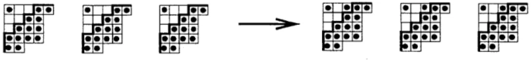
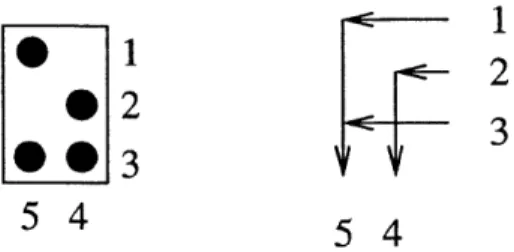
Definition 1.3.3 ([9], Definition 6.3). A F-graph is obtained from a J-diagram in

the following way. Place a vertex at the middle of each step in the boundary path

Figure 1-1: Example of a J-diagram and a F-graph

the boundary vertices. Now for each dot inside the J-diagram, draw a horizontal line to its right, and vertical line to its bottom until it reaches the boundary of the diagram. Then orient all vertical edges downward and horizontal edges to the left.

The source set of the F-graph is given by I(A) and the sink set is given by [n] \I(A).

Definition 1.3.4. A path in a F-graph is a directed path that starts at some

bound-ary vertex and ends at some boundbound-ary vertex. Given a path p. we denote its starting point and end point by p" and pe. A VD-family is a family of paths where no pair of paths share a vertex.

A dot at (i,

j)

j)

j

j)

Given a VD-family of paths {p1,..., pt}, we say that this family represents J

I(A)

\

The following proposition follows as a corollary from ([9]. Theorem 6.5).

Proposition 1.3.5 ([9], Theorem 6.5). Given a i-diagram L, let ML be the set that consists of J's such that J is represented by a VD-family in the F-graph of L. Then ML is a positroid, and this correspondence gives a bijection between J-diagrams and positroids.

IL1

F

n

Figure 1-2: Rules of the road for F-graphs

The following theorem described how to recover a decorated permutation from a J-diagram.

Theorem 1.3.6 ([9], Corollary 20.1). Define a map x that sends a J-diagram L to a decorated permutation 7r: = (r, col) according to the following rules: Inside the 17-graph of L, whenever we start at a boundary vertex i and reach

j

j.

edge, col(i) = 1 if otherwise. Then x is a bijection between i-diagrams and decorated

permutations.

For example, let us look at the J-diagram and F-graph of Figure 1-1. If we start at the boundary vertex 3, we end up at 10 by following the rules of the road. So we get 7r(3) = 10. If we repeat the procedure for all boundary vertices, we get

r = [2, 6, 10, 7, 3, 9,4, 1, 5,8].

1.4

Plabic graphs

In this section, we will review plabic graphs. Just like the fact that wiring diagrams represent a permutation, plabic graphs represent a decorated permutation. and hence positroids. Later in chapter 3, we will use these graphs to represent some special

collections called weakly separated collections.

Definition 1.4.1. A planar bicolored graph, or simply a plabic graph is a

planar undirected graph G drawn inside a disk. The vertices on the boundary are called boundary vertices, and are labeled in clockwise order by [n]. All vertices in the graph are colored either white or black. The boundary vertices have degree 1.

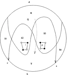
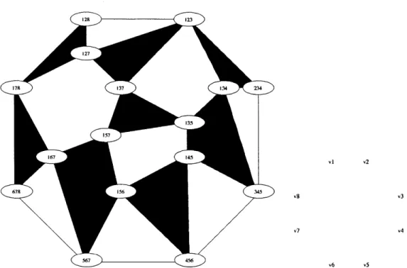
Figure 1-3: Labeling faces of a plabic graph

strands, within the disc D, each starting from and ending at a boundary vertex of

G.

Definition 1.4.2. The construction in this definition is depicted in Figure 1-3; the numeric labels in that figure will be explained below. The strands are drawn as follows: For each edge of G, draw two strand segments. If the ends of the segment are the same color, then the two strands should be parallel to the edge without crossing, and should run in opposite directions. If the two ends are different colors, then the two strands should cross, with one running towards each endpoint. Around each vertex, connect up the ends of the strands so that they turn right at each black vertex and left at each white vertex. We will have n strands leading from the boundary vertices to themselves., plus possibly some loops in the interior of G.

For most purposes, since contracting an edge whose vertices are colored in the same manner does not change the topology of the strands, we can reduce to the case that G is bipartite.

A plabic graph is called reduced [9, Section 131 if the following holds:

1. The strands cannot be closed loops in the interior of the graph.

2. No strand passes through itself. The only exception is that we allow simple loops that start and end at a boundary vertex i.

3. For any two strands a and

#,

#

B, then one strand, say a, is directed from A to B, and the other strand , is

directed from B to A. (That is the crossings of a and ,B occur in opposite orders in the two strands.)

The strand which ends at the boundary vertex i is called strand i.

Definition 1.4.3. [9, Section 13] For a reduced plabic graph G. let -KG E S, be

the permutation such that the strand that starts at the boundary vertex i ends at the boundary vertex 7G(i). A fixed point WG(i) = i corresponds to simple loop at

the boundary vertex i. We color a fixed point i of wG as follows: col(i) = 1 if the corresponding loop is counter-clockwise; and col(i) = -1 if the loop is clockwise. In this way, we assign the decorated strand perrmutation ir (7G, col) to each reduced plabic graph G.

There is a way to label the faces of a reduced plabic graph with subsets of [n]; this idea was first published in [12]. By condition 2 each strand divides the disk into two parts. For each face F we label that F with the set of those i

E

When we pass from one face F of G to a neighboring one F', we cross two strands. For one of these strands, F lies on its left and F' on the right; for the other F lie on the right and F' on the left. So every face is labeled by the same number of strands as every other. We define this number to be thc rank of the graph.

We define the boundary face at i to be the face touching the part of the disk between boundary vertices i - 1 and i in clockwise order. Let Ii be the label of that

is obtained from I by deleting i and adding in 7r (i); we deduce that (11. ... , I) is the

Grassmann necklace I(r).

We now describe how to see mutations in the context of plabic graphs. We have following 3 moves on plabic graphs.

(Ml) Pick a square with vertices alternating in colors, such that all vertices have degree 3. We can switch the colors of all the vertices. See Figure 1-4.

Figure 1-4: (M1) Square move (M2) For two adjoint vertices of

vertex. See Figure 1-5.

the same color, we can contract them into one

Figure 1-5: (M2) Unicolored edge contraction

(M3) We can insert or remove a vertex inside any edge. See Figure 1-6.

0

Figure 1-6: (M3) Middle vertex insertion/removal

The moves do not change the associated decorated permutation of the plabic graph, and do not change whether or not the graph is reduced. The power of these moves is reflected in the next Theorem:

Theorem 1.4.4. [9, Theorem 13.4] Let G and G' be two reduced plabic graphs with the same number of boundary vertices. Then the following claims are equivalent:

" G can be obtained from G' by moves (Ml)-(M).

Moves (M2) and (M3) do not change F(G), while move (M1) changes F(G) by a mutation.

Notice also that the moves (M1)-(M3) do not change the number of faces of the plabic graph. So all reduced plabic graphs for a given decorated permutation have the same number of faces. This number is given by the following theorem:

Theorem 1.4.5. Let G be a reduced plabic graph with decorated permutation 1r. Then G has ffr:) + 1 faces.

Proof. By [9, Theorem 12.7], S" is isomorphic to RIF(G)-1. And by

Chapter 2

Positroids and Schubert matroids

In this chapter, we give a purely combinatorial definition of a positroid. Recall that positroids are defined as matroids that can be realized by matrices that have non-negative maximal minors. We will show that positroids can be defined without using matrices: they can be defined as some collections satisfying certain cyclic inequalities. This part is based on [6].

2.1

Introduction

Let [n] {1, n} and let

(n])

some t E [n]. We define the ordering <t on [n] by the total order t <t t + 1 <t ... <t

n <t 1 <t -.. <tt-1. For I,JE ([]), where

I1 = {ii, . .. , i i}, ii <t i2 <t - - - <t ik

and

J= {1,. - - -, jk),ji <t j2 <t ... <t ik,

we set

For each I E

(1)

as

SMt:=

{J

E

|I <

J}.

For example, SMiJ in

(1)

Theorem 2.1.1 ([9], Theorem 17.2). Let St" be a nonnegative Grassmann cell, and let IM = (1,. In) be the Grassmann necklace corresponding to M. Then

n

Smt"

Qi

where Q'} _{is the cyclically shifted Schubert cell, which is the set of elements V G Grkn}

such that I is the lexicographically minimal base of My with respect to ordering <j on [n].

This result implies that:

Corollary 2.1.2. Let M be a positroid and let IM = (I1,.. In) be the associated Grassmann necklace. Then

n

M ; SMi, .

i=1

So the bases of a positroid are included in an intersection of cyclically shifted Schubert matroids. But we do not yet know if they are actually equal. Postnikov therefore conjectured that each positroid is exactly the intersection of cyclically shifted Schubert matroids. This is what we are going to prove in this chapter:

Theorem 2.1.3. M is a positroid if and only if for some Grassmann necklace

(1,) . .. , In),

n

M = SM .

i=1

In other words, M is a positroid if and only if the following holds : H E M if and only if H >t It for all t r [n].

3 2 4 5 8 7 6

10 9

Figure 2-1: Labeling the boxes inside the boundary strip

2.2

Connections between a J-diagram and a

Grass-mann necklace

Recall that each J-diagram corresponds to a positroid, and hence a Grassmann neck-lace. Given a J-diagram L, let us try to find out its corresponding Grassnann necklace

I= (11, . .. , I,) directly from the diagram. It is obvious that 1 = I(A).

For each box (x, y) in L, we can get a maximal chain (xt, yt) < -- (xi, yi) such that (xi, y1) is the unique dot in {(ij)Ji < xj > y} that minimizes x - i and

j

collection of hook paths at (X,, yr) for 1 < r < t is a VD-family. So we get J,) :=

I, \ 1 -x--, xt} U {yi, ... yt} E ML- In Figure 1-1, chain rooted at (5,9) is given by

(1, 10) < (5,9). A chain rooted at (3, 9) is given by (1, 10).

We define the boundary strip of a Young diagram to be the collection of boxes that touches the boundary path of the diagram. Look at the box that is uppermost and rightmost among the boxes in the strip. This box is adjacent to a vertical boundary path, and if that path is labeled with

j,

j

increase the label as we go downwards and to the left. In other words, if

j

j

j

j

j,

j

In the following proposition, we will show that a chain rooted at box labeled

j

Proposition 2.2.1. Fix a i-diagram L of shape A and let I = (I1, .... I,) be the

Grassmann necklace of ML. Let (x,y) be the box labeled

j

j,

Proof. Let F be a VD-fanily that represents Ij. Then F only contains paths that satisfy pS <

j <

any path p E F has to pass through a dot in the region

{(i,)

<

Let the chain rooted at (x, y) be (it,jt)<-

.

, ji).

hook path at (ir, jr) by pr. Then F must contain pi. If not, then Ij g, I(A)\{ii}U{j1}

because pS < iIp' > ji for all p E F. If pi,*. . p,. E F, then we also have pr+1 E F because if not, we get

hI

for any path p E F \

{pi,..

get F = {pi, ... ,pt} and Ih = J(xy).

In the case where there is no box labeled with

j,

_j

p'. This implies that I is represented by an empty family, so

we have Ij = I(A). 0

Let us look at an example. In the J-diagram of Figure 1-1, 14 is given by J(₃.6).

Chain rooted at (3,6) is given by (1,10) < (3,6). So 14 = 11 \ {1, 3} U {10,6} = {4, 5, 6, 8. 10}. 19 is given by Js,9). Chain rooted at (8,9) is given by (5, 10) < (8,9).

So 19 = 11 \ {5, 8} U {9, 10} = {1, 3, 4.9, 10}.

2.3

Proof of the main theorem

In this section, we will prove the main theorem by showing that for each Grassmann necklace I = (I1,..,I), we have

fl

that each J E

fl

In order to accomplish this, we will start from a full-J-diagram and use induction by increasing the number of empty boxes.

SMIJ()-*

@0

1 00 1

Figure 2-2: How the middle path is defined inside a J-diagram.

Proof. We need to show that for all J E SM(Ap), we have J E ML. Due to the definition of 1, there is a unique bijection

#

any a, b E I(A) \ J, the two intervals [a,

#(a)]

#(b))

\

(a,

#(a)).

Given any i-diagram L_ with associated Grassmann necklace I =

(1....,

|I1 \

Ia'|

$

Let us first assume that there exists an empty box in the boundary strip of L1.

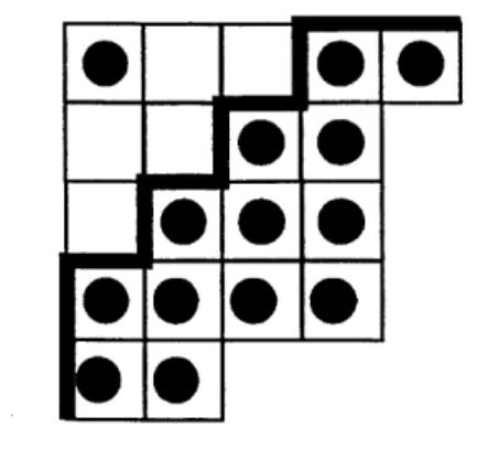
Consider an empty box b in the strip such that there is no empty box to its right or bottom. Then adding a dot to this box b will change exactly one element of the Grassmann necklace, since among the chains rooted at one of the boxes in the boundary strip, only the chain rooted at b is changed. So we only need to consider the case when all the boxes of the boundary strip are filled. We define the middle

path of LI to be a lattice path inside the diagram such that:

1. all boxes between the middle path and the boundary path are filled with dots,

2. the corner boxes of the upper region is empty. Upper region is the diagram obtained by looking at the boxes above or left of the middle path. A box is a

corner box of a diagram if there is are no boxes to its right and below.

Example of a middle path is given as a thick line in Figure 2-2.

Now., putting a dot into any corner box of the upper region will work. The reason for this is similar as the previous case, since exactly one chain among the chains

Figure 2-3: How the rooted chains change after a new dot is added.

rooted at boxes in the boundary strip is going to change, which implies that only one element of the Grassmann necklace is going to be affected by the newly added dot. This phenomenon is illustrated in Figure 2-3.

Proposition 2.3.2. Given any Grassmann necklace I= (I, .... In), we have M1

fl"

Proof. We will prove the proposition by induction on m, the number of empty boxes inside the J-diagram L1 of Mz. When m = 0, this is the full J-diagram case. So

assume for the sake of induction that we know the result for J-diagrams having < m empty boxes.

Use the construction above to obtain L-,, where

T

a

E [n]

Ia'|

tells us that

Mr,

fl>

Let (wq+r, zq+r) < .. < (Wq, zq) < ... < (wi, zi) _{be the chain representing I' in L11,}

such that (wq, zq) is the newly added dot going from L1 to L1,. In Lrv, we have dots

at (Wa, Zb) for 1 < a, b < _{q. Any VD-family Fj representing some J}

c

should contain a path in which (Wq, Zq) is a NW-corner.

In Fj, denote the path going through (wq, zq) by P. If there is no path in FT that

passes (wq-1, _{zq_1), we can pcrturb the path Pg to go through the points (wq, zq-1),} (Wq1. zq_1), (Wq, Zq) instead of going through (wq, Zq). So there must be a path Pq-1

E

is also a NW-corner of Pq-1. Repeating this argument, we getpg ... pi E FT each having (wq, zq), ... , (wi, zi) as a NW-corner.

Let (Xt, Yt) < . < (xi, yi) be the chain rooted at (wq, zq) in L1. Then

represents Ih in L₁. We have t > r due to the J-property. We want to show that

J g0 I0.

If p <, y1 or p" >a x1. then we have J I, and we are done. So let us assume,

Pe a y1 and p,5 a xi. If there is no path going through (xi, y1) in Fj, the path Pq

can be slightly changed so it goes through (xi, yi) and this path cannot have (wq, zq)

as its NW-corner. So there must be a path Pq+1 in Fj that passes through (x1, yi).

Due to similar reasons, we only need to consider the case when p1+1 >a Y2 and

p+ a x2. If there is no path going through (X2, y2) in Fj, the path Pq+1 can be

slightly changed so it goes through (x2, y2). This path cannot pass (Xi, yi), since we have X2 <0 x1 and Y2 >o Yi1 So there must be a path Pq+2 E .Fj that passes through

(x2, Y2). Repeating this argument, we get Pq+1. Pq+t c Ti. Then {p'+t, ...

PI}

So we have shown M1v \ Mx C SMy, \ SM., and we are finished. 0

Let us look at an example on using the main theorem. Let M be a positroid such that its Grassmann necklace is given by:

I1 = {1, 2,4},12 = {2,4,5},13 {3,4,5},1 4 = {4.5,2}, 15 = {5,1,2}.

Our main theorem tells us that:

M =

>1 11, H

...

H

= {{1,2,4},{1, 2, 5},{13, 4},{1,3,5},{2,4,5},{3,4,5}}.

2.4

Decorated permutations and the Upper

Grass-mann necklace

In the previous section, we have shown that a positroid is a collection given by setting cyclic lower boundaries. In this section, we will show that we can instead set cyclic

upper boundaries to get the same collection. Dual Schubert matroids will play the role of setting upper boundaries, just as Schubert matroids played the role of setting the lower boundaries. In other words, in this section, we will show that a positroid is also an intersection of cyclically shifted dual Schubert matroids.

Definition 2.4.1 ([9], Definition 13.3). A decorated permutation 7r: = (7r, col) is a

permutation 7r C S,, together with a coloring function col from the set of fixed points

{il7r(i)

points colored in two colors.

It is easy to see the bijection between necklaces and decorated permutations. To go from a Grassmann necklace I to a decorated permutation r: = (wr cot),

" if i+1 = (I\{i}) U {j}.

j

/

j,

* if 1

i+1 = i and i V Ii then 7r(i) = i, col(i) = 1.

* if Ii+1 =Ij and i

E I then gr(i) =i,col(i)

To go from a decorated permutation 7r = (7r, col) to a Grassmann necklace I,

Ii = {j E [nij <j 7r~1(j) or (7r (j) =

j

Let us look at an example. Given a Grassmann necklace I1 =

{1,

{2, 4, 5, 13 = {3, 4, 5}, 14 {4 5, 2}, I5= {5, 1. 2}, the associated decorated permu-tation is 7r = 53214.

Definition 2.4.2. For I = (i i....i) E

),

Schu-bert matroid SMi consists of bases H = (j1 .... ,jA) such that I >j H.

Fix a decorated permutation 7r: = (Ir, col). Let I,: = (I1,... , I,,) be the

corre-sponding Grassmann necklace and M,: the correcorre-sponding positroid.

Proof. In this proof, we will show that for any H E M,:, we have H

<1

proof for other inequalities is similar. Denote 1i = {ii, i} where i1 ... ,ik are

labeled in a way that satisfies r-1(ii) < ---<

Denote elements of H by hi < - < hk. Let j be the biggest element of [k] such

that:

1. ht ; 7r-

'(it)

2. hj > 7r-'(ij).

Since hj E (7r-1 (ij),r-1_(ij+

1)], we have we have {ii,...,i } C Ih. We get

IH n

n

The collection (J1 := r-1(I1),..., J, := r1 (In)) forms a necklace in the sense

that Ji+1 = Ji \ {7r-'(i)} U {i} except for i such that ir(i) = i. We will call this the

upper Grassmann necklace of ir.

To go from a decorated permutation i: (7r, col) to an upper Grassmann necklace

J, = {i E [n]|7r(i) <r i or (7r(i) = i and col(i) = -1)}.

Define

M:

n

.Sr: = S~.

=1

Lemma 2.4.3 tells us that M,:

c

Lemma 2.4.4. For any H E M,:, we have H >j 7r(J) = Ii for all i C [n].

As a consequence of this lemma we obtain the following result:

Theorem 2.4.5. Pick a decorated pernutation 7r: = (7r, col). Let I = (I1 .. ... In) and 3 = (J1, ... , J,) be the corresponding Grassmann necklace and the upper Grassmann

necklace. Then Ji = gr-1(Ii) for all i E [n]. We also have the equality:

n n

flSMi

SM .

i=1 i=1

For example, let us look at the positroid

M = {{1, 2,4}{1, 2, 5},{1,3,4},{13,5},{2,4 5},{3,4,5}},

whose associated Grassmann necklace is 11 = {1, 2, 4}, 2 = {2, 4, 5},13 = {3, 4, 5}, 14 = {4, 5, 2}, 15 = {5, 1, 2} and the decorated permutation is ir = 53214. Using Ji =

we get J1 = {3, 4, 5}, J2 = {3,5,1},J3 = {5,1,2},J4 = {5,1,3},J5 =

{1, 3,4}. Theorem 2.4.5 tells us that M = {HIH <1 J1,..., H 5 J5}.

2.5

Further Remark

Positroids correspond to the matroid strata of the nonnegative part of the Grassman-nian. Flag matroids correspond to the matroid strata of a flag variety.

Definition 2.5.1. A flag F is a strictly increasing sequence

F cF 2 _{C -.. c Fm}

of finite sets. Denote by ki the cardinality of the set F. We write F = (F',... Fm). The set F' is called the i-th constituent of F.

Theorem 2.5.2 ([2]). A collection F of flags of rank (ki,..., km) is a flag matroid if and only if:

1. For all i

E

E

2. For every w

.E

3. Every flag

B1 c -.. c Bm

Definition 2.5.3. A flag positroid is a flag matroid in which all constituents are

positroids.

It would be interesting to check what is the necessary condition for two decorated permutations, so that the corresponding positroids are concordant.

Chapter 3

Maximal weakly separated

collections and Plabic graphs

In this chapter, we study maximal weakly separated collections. Weak separation is a condition on pair of sets that first appeared in Leclerc and Zelevinsky's work describing quasicommuting families of quantum minors. They conjectured that all maximal by inclusion weakly separated collections of minors have the same cardinality (the purity conjecture), and that they can be related to each other by a sequence of mutations. We link the study of weak separation with total positivity on the Grassmannian, by extending the notion of weak separation to positroids. By using plabic graphs, we generalize the results and conjectures of Leclerc and Zelevinsky, and prove them in this more general setup. This part of my thesis is based on joint work with Alexander Postnikov and David Speyer [8].

3.1

Introduction

Leclerc and Zelevinsky [4], in their study of quasicommuting families of quantum minors, introduced the notion of weakly separated sets.

Let I and J be two subsets of [n]. Leclerc and Zelevinsky defined I and J to be weakly separated if either

I -< J \ I -< 12, or

2. |Jj 5

111

U

J1 -<I \ J -< J2,

where A -< B indicates that every element of A is less than every element of B. Leclerc and Zelevinsky proved that, for any collection C of pairwise weakly sepa-rated subsets of [n], one has

ICI

(')

Purity Conjecture.

Conjecture 3.1.1. [4] If C is a collection of subsets of [n], each of which are pairwise weakly separated from each other, and such that C is not contained in any larger

collection with this property, then |C| =

(n)

The above notion of weak separation is related to the study of the Pl6cker co-ordinates on the flag manifold, see [4]. Similarly, Scott [11] proved that, for any collection C C

([]) of pairwise weakly separated k element subsets on [n], one has

|CI < k(n - k)

+

coordinates on the Grassmannian. When

III

IJI,

becomes invariant under cyclic shifts of [n]. Indeed, in this case I and J are weakly separated if and only if after an appropriate cyclic shift (I \ J) -< (J \ I).

Moreover, Scott made the following conjecture.

Conjecture 3.1.2. /11] If C

c

([I)

ICI

We present a stronger statement, which implies both Conjectures 3.1.1 and 3.1.2.

Theorem 3.1.3. Let I, M and 7r be a Grassmann necklace, positroid and decorated permutation corresponding to each other. Let C C

(

ICI

(7r).

We will call collections C satisfying the conditions of this theorem maximal weakly separated collections inside

M.

This result implies Conjectures 3.1.1 and 3.1.2, and also the w-chamber conjecture of Leclerc and Zelevinsky [4], and their conjectures on mutations.

In particular, Scott's Conjecture 3.1.2 is the special case of our main result in the case where we look study the largest cell in the totally nonnegative part of the

Grassmannian.

We also prove the following result on mutation-connectedness, whose special cases

were conjectured in [4] and [11].

Theorem 3.1.4. Fix a positroid M. Any two maximal weakly separated collections inside M can be obtained from each other by a sequence of mutations of the following forr: C i-* (C

\{Sac})

a, b, c, d in [n] \S, C contains Sab, Sbc, Scd, Sda and Sac. (Here Sab is a shorthand

for S U {a, b}, etc.)

Our main tool is by showing that weakly separated collections and reduced plabic graphs are in a bijective correspondence.

Theorem 3.1.5. Fix a positroid M and the corresponding Grassmann necklace I. For a reduced plabic graph G associated with M, let F(G) C

(')

of labels of faces of G. Then the map G '-+ T(G) is a bijection between reduced

plabic graphs for the positroid M and maximal weakly separated collections C such that I C C C M.

Theorems 3.1.3 and 3.1.4 follow from the correspondence in Theorem 3.1.5 and the properties of plabic graphs from [9].

3.2

Weakly separated collections

In this section, we define weak separation for collections of k element subsets and discuss the k subset analogue of Leclerc and Zelevinsky's conjectures. The relation

of this approach to the original definitions and conjectures from [4] will be discussed in section 3.8. We will also define weakly separated collections inside positroids.

Lot us fix two nonnegativc integers k < n.

Definition 3.2.1. For two k element subsets I and J of [n], we say that I and J are weakly separated if there do not exist a, b, a'. b', cyclically ordered, with a, a' e I

\

We write I || J to indicate that I and J are weakly separated.

We call a subset C of

(n)

c

We define a maximal weakly separated collection to be a weakly separated collection which is not contained in any other weakly separated collection.

Following Leclerc and Zelevinsky

[4],

Proposition 3.2.2. [11], cf. [41 Let S E ("_) and let a, b, c, d be cyclically ordered elements of [n] \ S. Suppose that a maximal weakly separated collection C contains

Sab, Sbc, Scd, Sda and Sac. Then C' := (C \ {Sac}) U {Sbd} is also a maximal weakly separated collection.

We define C and C' to be mutations of each other if they are linked as in Proposi-tion 3.2.2.

We now define the notion of a maximal weakly separated collection inside a positroid.

Definition 3.2.3. Fix a Grassmann necklace I (I1. In), with corresponding

positroid MI. Then C is called a weakly separated collection inside MI if C is a weakly separated collection and I C C C Mr. We call C a maximal weakly separated

collection inside MI if it is maximal among weakly separated collections inside M. The following lemma guarantees us that there exists a maximal weakly separated collection for any positroid.

Lemma 3.2.4. For any Grassmann necklace I, we have I C ME, and I is weakly separated.

Proof. For every i and

j

iI

By the definition, Ir+1 is obtained from I, by deleting r and adding another element, or Ir+1 = 1r. As we do the changes I, -+ 12 -+ - - - -+ In -+ 1, we delete

each r E [n] at most once (in the transformation 1, -+ Ir+1). This implies that we

add each r at most once.

Let us show that Ij \ i J [ji). Suppose that this is not true and there exists r E

(Ih \

ii)

n

j).

Grassmann necklace, or r does not belong to all elements of the necklace.) Consider

the sequence of changes I -+ 1 +

j -+ - - -r -* r+1 -+ - - --+ Ij. We should have

r I Ii, r E I., r V Ir+1, r E Ij. Thus r should be added twice, as we go from i to Ir

and as we go from Ir+1 to 1. We get a contradiction.

Thus Ij \ i 9 [j, i) and, similarly, I \ Ij 9 [i, j). We conclude that Li i Ii and

i

Then our main result can be described as:

Theorem 3.2.5. Fix any Grassmann necklace I. Every maximal weakly separated collection inside M₁ has cardinality f(I) + 1. Any two maximal weakly separated collections inside

M

The above result follows naturally from the following claim, that establishes a correspondence between maximal weakly separated collections in a positroid and re-duced plabic graphs. It describes maximal weakly separated collections as labeled sets F(G) of reduced plabic graphs.

Theorem 3.2.6. For a decorated permutation 7f and the corresponding Grassmann necklace 1 = I(,r), a collection C is a maximal weakly separated collection inside the positroid Mz if and only if it has the form C = F(G) for a reduced plabic graph with

strand permutation r: .

In particular, a maximal weakly separated collection C in

('])

3.3

Decomposition into connected components

M

The connected components of 7r:, I, and

M

Example 3.3.1. Take the decorated permutation 7r: where ir is given by 31254. Then the connected components are 123 and 45.

Definition 3.3.2. Let [n] = S1 U S2 U ... U Sr be a partition of [n] into disjoint

subsets. We say that [n] is noncrossing if, for any circularly ordered (a, b. c, d), we have {a. c} 9 Si and {b.d} Sj then i = j.

Since common refinement of two noncrossing partitions is noncrossing, we can define the following:

Definition 3.3.3. Let 7r: be a decorated permutation. Let [n] = [_ Si be the finest noncrossing partition of [n] such that, if i E S then wr(i) E Sj.

Let 7r be the restriction of 7r: to the set Si, and let I() be the associated Grass-mann necklace on the ground set Sj, for

j

We call 7r the connected components of 7r=, and I j) the connected components

of I.

We say that 7r: and I are connected if they have exactly one connected component.

Lemma 3.3.4. The decorated permutation ir: is disconnected if and only if there are two circular intervals [i, j) and [j, i) such that 7r takes [i,

i)

preserved by 7r. So there is a nontrivial noncrossing partition preserved by r and r is not connected. Conversely, any nontrivial noncrossing permutation can be coarsened

to a pair of intervals of this form so, if 7r is disconnected, then there is a pair of

intervals of this form. 0

Note that each fixed point of 7r: (of either color) forms a connected component.

Lemma 3.3.5. A Grassiann necklace I = (11, .. ., ) is connected if and only if the

sets I1,..., In are all distinct.

Proof. If ir: is disconnected then let [i, j) and [j, i) be as in Lemma 3.3.4. As we change from Is to Ii+1 to Ii+2 to ... to I1, each element of [i,

j)

Conversely, suppose that I = Ij. As we change from i to I+1 to 'i+2 to ... to Ij,

each element of [i.

j)

j)

In this section, we will explain how to reduce computations about positroids to the connected case.

So, for the rest of this section, suppose that 1i = Ij for some i / j. Set 11:=

[i,

j) n

[j,

i)

n

Ii;

1121.

I[i,j)|

and n

_i)

Proposition 3.3.6. For every J E M, we have |Jf

[i.j)|

(in

[j,i)|

Proof. Since Ii is the <j minimal element of M, we have

|[ij)

nil

|[i,j)

n

ii|

for all J E M. But also, similarly,

|[j,i)

ni

J|

l [ji) n-i

Ig|

k2

Adding these inequalities together, we see that