Modelling and Linear Control of a Buoyancy-Driven Airship

HAL Id: hal-00405211

https://hal.archives-ouvertes.fr/hal-00405211

Submitted on 20 Jul 2009

HAL is a multi-disciplinary open access

archive for the deposit and dissemination of

sci-entific research documents, whether they are

pub-lished or not. The documents may come from

teaching and research institutions in France or

abroad, or from public or private research centers.

L’archive ouverte pluridisciplinaire HAL, est

destinée au dépôt et à la diffusion de documents

scientifiques de niveau recherche, publiés ou non,

émanant des établissements d’enseignement et de

recherche français ou étrangers, des laboratoires

publics ou privés.

Modelling and Linear Control of a Buoyancy-Driven

Airship

Xiaotao Wu, Claude Moog, Yueming Hu

To cite this version:

Xiaotao Wu, Claude Moog, Yueming Hu. Modelling and Linear Control of a Buoyancy-Driven Airship.

The 7th Asian Control Conference, Aug 2009, Hong Kong, China. pp.6. �hal-00405211�

Modelling and Linear Control of a Buoyancy-Driven Airship

Xiaotao WU Claude H. MOOG and Yueming HU

Abstract— We describe the modelling and control of a new-kind airship which is propelled by buoyancy. Based on the Newton-Euler equations and Kirchhoff equations, and referred to the models of underwater gliders and aircraft, a 6DOF nonlinear mathematical model of a buoyancy-driven airship is derived, with features distributed internal mass, and no thrust, elevators and rudders. The attitudes are controlled by the motion of internal mass. The performances of the airship are studied in the vertical plane. A linear feedback controller is derived for the nonlinear model. The results of simulation display robustness properties of the controllers to disturbances.

I. INTRODUCTION

Stratospheric platforms or high altitude platforms, which locate 17-22 km above the ground, and keep quasi-geostationary positions, attract an increasing research interest for these recent ten years. Such a platform has the potential capability to serve as a wireless communication relay station and as a high resolution observing station [1], [2], [3].

A high altitude unmanned airship as this platform has the following features; driven by solar power makes it long-endurance in high altitude, and generally this platform can take 1000 kg to 3000 kg payload which is a low cast methods to carry out similar functions of satellites. A conventional airship is driven forward by propulsors along the hull, the attitude is controlled by elevators and rudders or vector-propulsors. O e1 e2 e3 G i j k b R Helium Ballonet Ballonet Exhaust Valve Blower Ballast

Fig. 1. Structure of Buoyancy-Driven Airship

Buoyancy-driven airships move forward by a cyclic change of the net buoyancy of the craft and of the position of ballast. This concept of airship comes from underwater gliders who replace traditional thrust propulsion by a cyclic

This work was supported by CSC

X. WU is with Institut de Recherche en Communications et Cybern´etique de Nantes, 1 rue de la No¨e, 44321, Nantes, France, and South China

University of [email protected]

C. H. MOOG is with Institut de Recherche en Communications et

Cy-bern´etique de Nantes,[email protected]

Y. HU is with South China University of Technology,

[email protected]

change of the net buoyancy and of the position of the centroid, which has been proved to be efficient in water [4]. Underwater gliders cruise for long distances consumed little power. The structure of this new-kind airship see Figure 1. The blower is used to fill an impermeable inner bladder with ambient air, and the valve is used to release the inner air. The ballast can move in the horizontal plane.

V o (G) i e1 θ ξ α e3

Fig. 2. Ascent of the Buoyancy-Driven Airship

The mechanism of operating this kind of airship is as follows. When releasing air from ballonets, the mass of the airship reduces, the lift becomes positive. Accompanying the ballast moves to the tail, the airship gets a positive pitch angle θ, and moves upward and forward, see Figure 2. Oppositely, when pumping air into ballonets, the airship mass increases, the lift decreases and becomes minus. Accompanying the ballast moving to the head, the airship gets a negative pitch angle θ, and moves downward and forward, see Figure 3. If the ballast is moving to side, then the airship will roll. Due to the coupling of roll and rotation moments, the airship flies to the right or the left.

o

Fig. 3. Descent of the Buoyancy-Driven Airship

The environment of high altitude is quite different from underwater. Comparing with incompressible water, air is compressible. The density, temperature, and pressure of atmosphere is changing with the change of altitude. All of this make high altitude airship have some differences from underwater gliders, and more difficult to control.

At present, most research on airship control is based on airships with actuators-thrusts and elevators [5]-[8]. Almost no paper discusses the possibility of airship driven by buoyancy, just as underwater gliders. The only monograph available on buoyancy-driven airship is the doctoral

disserta-tion [9]. This pioneering study includes the effect of various atmospheric conditions. However, the complete mathematical model of 6DOF is not given, and the control method also needs to be improved.

The contributes in the rest of this paper are as follows. The complete equations of 6DOF motion are given for the first time for a high altitude airship only driven by buoyancy. It includes the modelling of the ballast and the ballonets. This full model is derived from the model of the underwater glider. Dynamic performances have been studied, and a linear controller have been tested.

In section II, the mathematical model of a high altitude buoyancy-driven airship is derived. In section III, the model is specialized to the vertical plane. Then the nonlinear model has been linearized, the static stability and controllability has been analysed. In section IV, a LQR controller has been derived for the nonlinear system and the simulations are presented.

II. AIRSHIPDYNAMICMODELLING

A. Kinematics

Figure 1 shows the assignment of the two frames. The body frame {O, e1, e2, e3} is assigned with the reference point O at the center of hull, overlapped with the center of buoyancy CB. The inertial {G, i, j, k} frame is fixed to the earth, with the axis k along the direction of gravity [8]. To reduce the drag of the body, the hull of airship is designed to have a high volume/surf ace − area ratio. The shape comes from revolving of an airfoil profile. The airfoil profile can be chosen from NACA series of US. A ellipsoid has been used to represent that special shape for simple in this paper, and given that the equatorial radii and the polar radius are 7 m, 3 m and 3 m respectively.

The rotation matrix between the body frame and the inertial frame is represented by R1 which is composed by the pitch angle θ, the yaw angle ψ and the roll angle φ The position of the airship in the inertial frame is represented by vector b = (x, y, z)T _{∈ <}3_{, see Figure 1. R}

1∈ SO(3),

SO(3) is 3×3 special orthogonal matrix, defined as follows: SO(3) = {R1∈ <3×3|RRT = I, detR = 1} here I denotes a 3×3 identity matrix. The attitude and posi-tion of the airship is decided by (R1, b). So the configuration space of the system is defined as:

SE(3) = {(b, R1)|b ∈ <3, R1∈ SO(3)} = <3× SO(3)

SE(3) can be represented by homogeneous coordinates, as

follows: µ

R1 b

0 1

¶

∈ SE(3)

SE(3) is a rotation matrix group. For example, if G ∈ SE(3), then G is a transformation matrix of the rigid body from body frame to the inertial frame [10].

Let V = (v1, v2, v3)T and Ω = (Ω1, Ω2, Ω3) denote the velocity and the angular velocity in the body frame respectively. So the position and the attitude of the airship

can be described by the Lie algebra of SE(3), denoted as the group se(3). It is as follows:

µ ˆ Ω V 0 0 ¶ ∈ se(3)

Define the operator ∧ for a vector x = (x1, x2, x3)T ∈ <3, ˆ x =   _x0₃ −x₀3 _−xx2₁ −x2 x1 0  

and ˆx ∈ so(3), where so(3)is the Lie algebra of SO(3). The kinematics of the airship are given by

µ _˙ R1 ˙b 0 0 ¶ = µ R1 b 0 1 ¶ µ ˆ Ω V 0 0 ¶ (1) B. Mass Distribution and Definition

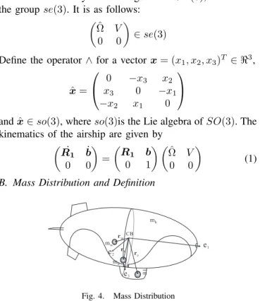
CB m rp mw r_w mb mh e1 e3 e2 rb

Fig. 4. Mass Distribution

The airship described in this paper is driven by the buoyancy and the ballast, just like some underwater gliders [11]. To set up the mathematical model, The entire mass of airship have to be splited into several terms. Let mh denote the uniformly distributed hull mass, mb is the variable mass of ballonets, ¯m is the mass of the inside movable ballast,

and mw denotes other inside fixed masses whose centroid offset from CB. rp = (rp1, rp2, rp3)T, rb and rw are the vectors from CB to the mass points of ballast, the ballonet and mw, see Figure 4.

The mass msis the total stationary mass, thus ms= mh+

mb+ mw. The total mass of the vehicle is mv, so we have:

mv = ms+ ¯m = mh+ mb+ mw+ ¯m. Let m = ρa∇ is the buoyancy of the airship with volume ∇. Thus, the net buoyancy of the airship is m0= mv−m. In this paper, mh= 269 kg, ¯m = 30 kg, and mw, rb and rw are neglected.

C. Fluid Inertia Forces and Added Mass

The inertia of airships with a large V olume/M ass ratio is much more significant in comparison with conventional airplanes. So, fluid inertial forces should be considered.

In the case of the motion of a rigid body in an ideal fluid with velocity vi in the direction i, the force acted on the rigid body by the fluid in the direction j is Rj = −mij˙vi and the parameter mijis called the added mass. There are 36 added masses for a rigid body in motion; the matrix Madd including those added masses is called the inertia matrix [5].

Madd= µ

Mf ∗

∗ Jf

¶

Mf is the symmetric 3 × 3 added mass matrix; Jf is the added inertia matrix; and the other two blocks are added

cross terms which are neglected. Here, It is supposed that the airship is centrosymmetric, so only elements on the diagonal are nonzero, other elements are zero because of symmetry. So, Mf = diag{m11 m22 m33} and Jf = diag{m44 m55 m66}. In this paper, m11 = 0.8mh, m33 =

mh and m55= 1.3Jyy. Jyy is the moment of inertia of the

airship around y axis, and approximately, Jyy = m(a2 + b2_{)/5 ≈ 3500 kg · m}2_.

In an ideal fluid, the kinetic energy Tadd of fluid

distur-bances is Tadd= 1 2 6 X i=1 6 X j=1 mijζiζj= 1 2(m11v 2 1+ m22v22 +m33v23+ m44Ω21+ m55Ω22+ m66Ω23) here ζ1 = v1, ζ2 = v2, ζ3 = v3, ζ4 = Ω1, ζ5 = Ω2, ζ6 = Ω3. The momenta B = (B1, B2, B3)T and moments of momentum K = (B4, B5, B6)T of fluid disturbances are related to the kinetic energy Tadd:

Bi= ∂Tadd ∂ζi (i = 1, 2, · · · , 6) So, B = Mfv K = JfΩ

So, the inertial forces FI and moments MI acting on the

airship are as follows

FI = −dB dt = −( d ˜B dt + Ω × B) = −Mf˙v + Mfv × Ω (2) MI = −dK dt = −( d ˜K dt + Ω × K + v × B) = −JfΩ + J˙ fΩ × Ω + Mfv × v (3) here, dB

dt, dKdt denote the time-derivative of momentum B

and angular momentum K with respect to the inertial frame,

d ˜B

dt and d ˜dtK denote the time-derivative in the body frame. D. Aerodynamic forces and moments

Different pneumatic pressures are distributed on the sur-face of a vehicle flying in the atmosphere. The effect of those pneumatic pressures can be presented by aerodynamic forces Fa and moments Maas follows,

Fa = (Xa, Ya, Za) Ma = (La, Ma, Na)

The aerodynamic forces are contributing by the forces and moments on the hull and fin and act on the center of buoyancy CB. By convention, the decomposed aerodynamic forces lie in the velocity frame (also called the wind frame), and the moments are decomposed in the body frame [6].

Drag : Xa= 1 2ρaV 2_(S hCx1+ SfCx2) Sidef orce : Ya= 1 2ρaV 2_(S hCy1+ SfCy2) Lif t : Za= 1 2ρaV 2_(S hCz1+ SfCz2) Roll moment : La= 1 2ρaV 2_(S hlh1Cl1+ Sflf 1Cl2) P itch moment : Ma= 1 2ρaV 2_(S hlh2Cm1+ Sflf 2Cm2) Y aw moment : Na= 1 2ρaV 2_(S hlh3Cn1+ Sflf 3Cn2)

here, ρa is the density of ambient air, Sh and Sf are the

reference areas of hull and fin, lh1, lh2, lh3 and lf 1, lf 2, lf 3

are the distances from the CB to the aerodynamic center of the hull and fin. The Ci’s are the aerodynamic coefficients

which are computed from wind tunnel experiments. Those coefficients do mainly depend on the angle of attack α and the sideslip angle β.

Since Fa is respected to the velocity frame, Fais

trans-ferred to the body frame, which denotes by Fat. Fat=



cos α cos β_{− sin β} cos α sin β_{cos β} − sin α₀ sin α cos β sin α sin β cos α



 Fa= R2Fa

(4) where R2 is the transfer matrix from the velocity frame to the body frame. Ma is respected to the body frame, so,

Mat= Ma (5)

E. Gravity and Buoyancy

In the inertial frame, the composite effect of gravity and buoyancy along the axis of inertial frame is denoted by FGB

as follows,

FGB = m0gk

where, k is a unit vector pointing in the direction of gravity. FGB is transferred to the body frame as follows,

FGBt= RT1FGB = m0gRT1k (6)

It is assumed that the centroid of the stationary mass ms

is on CB. So there is no moment which is caused by msand

the buoyancy of the airship. Only the ballast have moments since rp is not zero. In the inertial frame, the moment is

MGB = m0grs× k

which is transferred to the body frame as follows,

MGBt= RT₁MGB = m0gRT₁rs× k (7) F. Dynamics of the Ballast

Let rp be the position of the ballast in the body frame.

If the airship is rotating with angular velocity Ω. According to the relation between the absolute velocity and the relative velocity, the absolute velocity of the ballast in the body frame vp is as follows,

Let Bp = (Bp1, Bp2, Bp3)T denote the momentum of the

ballast, and u = (u1, u2, u3)T denote the total external force acting on the ballast. Both Bpand u are with respect to the

body frame. So that,

Bp = mv¯ p= ¯m(v + ˙rp+ Ω × rp) (8)

˙

Bp = u (9)

From (8), one gets, ˙rp= 1

¯

mBp− v − Ω × rp (10)

G. Model

Let Btotal and Ktotal be the total momentum and the

total moment of momentum of the airship. one gets,

Btotal = msv + Bp (11)

Ktotal = JsΩ + rp× Bp (12)

here Jsis the matrix of the moment of inertia of the airship.

Let Ftotaland Mtotal be the total external force and the

total moment of the airship. From equation (2) to (7), Ftotal

and Mtotal be computed as follows,

Ftotal= FI+ Fat+ FGBt (13)

= −Mf˙v + Mfv × Ω + +m0gRT1k + Fat

Mtotal= MI+ Mat+ MGBt (14)

= −JfΩ+ J˙ fΩ × Ω+ Mfv × v + m0gRT1rs× k + Mat

Similar to equation (2) and (3), Ftotal and Mtotal are

derived from (11) and (12) as follows, Ftotal=dBtotal dt = d ˜Btotal dt + Ω × Btotal Mtotal=dKtotal dt = d ˜Ktotal dt + Ω × Ktotal+ v × Btotal Substituted (9), (11) and (12) into above equations, then,

Ftotal= ms˙v + u + msΩ × v + Ω × Bp (15) Mtotal= JsΩ + ˙r˙ p× Bp+ rp× u − JsΩ × Ω

− msv × v + Ω × (rp× Bp) + v × Bp (16)

Substituted (10) into (16), then gets,

Mtotal = JsΩ − Ω × r˙ p× Bp+ rp× u − JsΩ × Ω

−msv × v − rp× Bp× Ω (17)

˙v is derived from (13) and (15) as follows, ˙v = M−1¡_{(M v + B}

p) × Ω + m0gRT1k + R2Fa− u

¢ (18) where, M = msI + Mf = diag(m1, m2, m3). I is the 3 × 3 identity matrix.

Similarly, ˙Ω is derived from (14) and (17) as follows, ˙

Ω = J−1_{((JΩ + r}

p× Bp) × Ω + Ω × rp× Bp

+ M v × v + ¯mgrp× RT₁k + Ma− rp× u) (19)

where, J = Js+ Jf = diag(J1, J2, J3).

As the airship is driven by change of buoyancy, it is necessary to control the mass of ballonets, through the input u4, as

˙

mb = u4 (20)

Combining with equations (1), (18), (19), (10), (9) and (20) , the mathematical model of a buoyancy-driven airship is obtained as           ˙ R1 ˙b ˙v ˙ Ω ˙rp ˙ Bp ˙ mb           =           R1Ωˆ R1v M−1_F¯ J−1_M¯ 1 ¯ mBp− v − Ω × rp u u4           (21)

where, ¯M is a moment matrix, and ¯F is a force matrix. The values of ¯M and ¯F is as follows,

¯

M = (JΩ + rp× Bp) × Ω + Ω × rp× Bp

+M v × v + ¯mgrp× RT₁k + Ma− rp× u

¯

F = (M v + Bp) × Ω + m0gRT1k + R2Fa− u

III. A SPECIAL CASE OF THE AIRSHIP DYNAMICS

A. Dynamics in the Vertical Plane

This mathematical model (21) has many complex cou-plings, which make it difficult to analyse by conventional ways as decoupling of the longitudinal plane and the lateral plane through decoupling [5]. Thus, we restrict the airship in the vertical plane.

The airship has to be driven by a periodic change of net buoyancy. The airship moves in a saw-tooth pattern path. So the most ideal and simplest condition is that the airship only moves in the vertical plane e1− e3 and it is assumed not to be disturbed by the wind and the atmosphere. Thus, it is assumed that there is no wind, and the density, pressure, temperature of atmosphere are constant; the vertical plane of the body frame and the inertial frame do coincide.

Since the airship only flies in the vertical plane, some states are set to zero. Thus, attitude angles ψ = φ = 0, position y = 0, velocity v2 = 0, angular velocities Ω1 = Ω2= 0. And we also suppose the ballast only move in the vertical plane, so rp2= 0, Bp2= 0 and u2= 0.

Substituting the above restricted conditions into the math-ematical model (21), the motion equations in the vertical

plane reduce to, ˙θ =Ω2 (22) ˙Ω2=1 J2((m3− m1) v1v3− (rp1Bp1+ rp3Bp3)Ω2+ Ma − ¯mg(rp1cos θ + rp3sin θ) + rp1u3− rp3u1) (23) ˙v1= 1 m1(−m3v3Ω2− Bp3Ω2− m0g sin θ + Xacos α − Zasin α − u1) (24) ˙v3= 1 m3 (m1v1Ω2+ Bp1Ω2+ m0g cos θ + Xasin α + Zacos α − u3) (25) ˙rp1=1 ¯ mBp1− v1− rp3Ω2 (26) ˙rp3=1 ¯ mBp3− v3+ rp1Ω2 (27) ˙ Bp1=u1 (28) ˙ Bp3=u3 (29) ˙ mb=u4 (30)

Here, the drag, lift and pitch moment in the vertical plane are simplified as follows,

Xa= 1 2ρa∇ 2/3_v2_(C x0+ Cxαα2) Za= 1 2ρa∇ 2/3_v2_(C z0+ Czαα) Ma= 1 2ρa∇v 2_(C m0+ Cmαα) B. A Nonlinear Feedback Controller

To keep control of the attitude and velocity of the airship, let new control input ˜u = (˜u1, ˜u2, ˜u3)T. Differentiating (22), with (24) and (25), then gives

  ¨ θ ˙v1 ˙v3   =  u_u˜_˜1₃ ˜ u4   = −P + C  u_u1₃ u4   ₍₃₁₎

Form differentiating (22), (24) and (25), matrices P and C can be derived. Thus, we can get nonlinear state feedback from (31),  u_u1₃ u4   = C−1    u_u˜_˜1₃ ˜ u4   + P   ₍₃₂₎

which linearizes ¨θ, ˙v1 and ˙v3 with respect to the new input ˜

u.

Substitute (32) into (24)-(30), and get the motion equations of the airship with a nonlinear states controller in the vertical plane. Results of (31) will be published elsewhere.

C. Static Stability Analysis

As Figure 5, the airship driven by buoyancy flies along an oblique line with angle ξe during equilibrium cruise. At

a time t, the airship is at the position (x, z) in the vertical plane with respect to the inertial frame, and (x0, z0) in the coordinate i0 − G − k0.

G

_i

ξ

Desired Flying Angle

ξ

x

z _z’

Fig. 5. Flying Sketch

According to the rotation matrix, the distance from the airship to the desired path is as follows, see Figure 6,

z0 = − sin ξex + cos ξez (33)

Differentiating (33) and substituting v1, v3 and θ into it. The perpendicular velocity to desired path is

˙z0 = − sin ξe(v1cos θ + v3sin θ)

+ cos ξe(−v1sin θ + v3cos θ) (34) During the equilibrium cruise, equations (24)-(30) and (33) are all equal to zero. Through those equations, the equilibrium states xe =

(θe, Ω2e, v1e, v3e, rp1e, rp3e, Bp1e, Bp3e, mbe, z 0

e)T and

input ue = (u1e, u2e, u3e)T during cruise under desired path angle ξe and speed Vecan be got.

The nonlinear model (22)-(30) can be simulated directly in MATLAB through the principle of digital integration, but the relation between parameters and performances of the system can not be clear revealed from the nonliear model. Thus, as conventional [5], small disturbance method is used to linearize the mathematical model around the equilibrium. The static stability of the airship around the equilibrium can be studied through the linearized model.

The motion of airship can be splited into two motions, the benchmark motion xe and ue which are the values on the

equilibrium, and the disturbing motion ∆x and ∆u which are the values away from the equilibrium. Substituting x = xe+ ∆x and u = ue+ ∆u into (22)-(30) and (34), the

result only keep the first-order of ∆x and ∆u, neglected high-order terms. Then, the linearized model is as follows,

∆ ˙x = A∆x + B∆u (35)

where, A is a 12 × 12 constant system matrix, and B is a 12 × 3 input matrix.

Given that the airship is desired to fly with the angler ξe= 15◦ and the volecity Ve= 10 m/s. After computered

the values of states on that equilibrium and linearization, the values of matrix A and B can be got. The eigenvalues of the system are not totally stable, but the system is controllable.

IV. LQR CONTROLLER OF THEAIRSHIP

In this section, we design a simple linear feedback con-troller for the nonlinear system (22)-(30), and demonstrate the performance of that controlled flying in the vertical plane. This simple linear controller is not good enough with large initial errors, and which need improve.

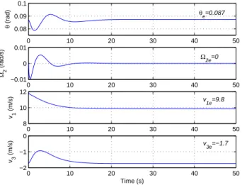
0 10 20 30 40 50 0.08 0.09 0.1 θ (rad) 0 10 20 30 40 50 −0.01 0 0.01 Ω2 (rad/s) 0 10 20 30 40 50 8 10 12 v1 (m/s) 0 10 20 30 40 50 −2 −1 0 v3 (m/s) Time (s) θ_e=0.087 Ω_2e=0 v 1e=9.8 v_3e=−1.7

Fig. 6. Simulation Result

The linear quadratic regulator (LQR) is a well-known design technique that provides practical feedback gains. It is assumed that all the 10 states ∆x are available for the controller. The infinite horizon cost function is defined as,

J = Z _∞

0 ¡

∆xT_{Q∆x + ∆u}T_R∆u¢_dt

The weight matrices Q and R are tuning parame-ters and their choice will decide about the performance of the closed loop system. In this simulation, Q = (2, 1, 2, 2, 1, 1, 1, 1, 0.5, 1)T_{, R = (0.1, 0.1, 0.1)}T_.

The feedback gain is a matrix K, implemented as, ∆u = −K(x−xdesired) = −K(x−xe) = −K∆x (36)

where, K is easily computed by MATLAB. Substitute the linear feedback controller (36) into nonlinear equations in the vertical plane (22)-(30). Given ξe = 15◦ and the

volecity Ve = 10 m/s, so αe = −10◦, v1 = 9.8 m/s and

v3= −1.7 m/s. If there is a abrupt wind led up to +2 m/s offset of v1. Figure 6 is the simulation of the nonlinear system with controller (36) under that initial errors, and Figure 7 is the flying path of the airship in this situation. The system can converge to the equilibrium after 15 seconds with that LQR controller. But the system will be unstable with larger initial errors.

V. CONCLUSION

In this paper, A novel airship has been studied, which is driven by a cyclic changing the net buoyancy of the airship, and the attitude is controlled by moving the internal ballast. There are not conventional thrusts, elevators and rudders.

Referred to the model of underwater glider, a full 6DOF nonlinear model of the airship has been derived with the ballast and the ballonet being considered separately. The mathematic model is similar to the model of underwater sliders, but it is derived by a general aerial way [8], [11]. The dynamics in the vertical plane has been derived. A

0 200 400 600 800 1000 0 50 100 150 200 250 300 x (m) z (m) Desired Path Flying Path

Fig. 7. Flying Path

nonlinear controller is designed. The nonlinear model in the vertical plane has been linearized, and the static stability and controllability of the airship have been studied. A LQR linear feedback controller also has been designed and simulated.

Compared to most of the prevalent high-altitude airship researches, this paper give out a novel concept of the high-altitude airship. Compared to the conventional engine-driven airship, the new kind airship is driven by buoyancy. This driving method aims at making the airship cruise long distant with consuming little energy.

Future research perspectives include the effects of the various atmospheric density, temperatures and pressure with the change of altitude based on this model, and the design of a better performance nonlinear controller. The dynamics in the lateral plane also need be considered.

REFERENCES

[1] A. Elfes and S. Bueno, Project AURORA: development of an

au-tonomous unmanned remote Monitoring Robotic Airship, J. Braz.

Comp. Soc. Vol. 4 no. 3, pp70-78, Apr.1998.

[2] T. C. Tozer and D. Grace, High-altitude platforms for wireless

commu-nications, IEE Electron. Commun. Eng. J., vol. 13, no. 3, pp. 127137,

Jun. 2001.

[3] Naval Research Advisory Committee, Lighter Than Air Systems for

Future Naval Missions Briefing: Flag Officers and Senior Executive

Service, The Pentagon Auditorium, Washington D.C., October, 2005. [4] Nonlinear gliding stability and control for vehicles with hydrodynamic

forcing, Automatica, 44, pp. 1240-1250, 2008.

[5] L. Beji and A. Abichou, Position and attitude control of an

under-actuated autonomous airship, International Journal of Differential

Equations and Applications, Volume 8, No. 3, pp. 231-255, 2003. [6] J. Mueller and M. Paluszek, Development of an aerodynamic model

and control law design for a high altitude airship, AIAA Unmanned

Unlimited Conference, No. AIAA-6479, Chicago, IL, 2004. [7] J. Ouyang, Research on modeling and control of an unmanned airship,

Dissertation for the Doctor Degree, Shanghai Jiaotong University, 2003.

[8] B. Gomes and J. G. Ramos, Airship dynamic modeling for autonomous

operation, IEEE Int. Conf. on Robotics and Automation, pp.

3462-3467, 1998.

[9] R. Purandare, A buoyancy-propelled airship, Dissertation for the Doctor Degree of Philosophy, New Mexico State University, 2007 [10] N. Leonard, Stability of a bottom-heavy underwater vehicle,

Automat-ica, Vol. 33, No. 3, pp. 331-346, 1997

[11] N. Leonard and J. Graver, Model-based feedback control of

au-tonomous underwater gliders, IEEE Journal of Oceanic Engineering,