NEAR DETERMINISTIC SIGNAL PROCESSING USING GPU, DPDK, AND MKL
ROYA ALIZADEH
D´EPARTEMENT DE G´ENIE ´ELECTRIQUE ´
ECOLE POLYTECHNIQUE DE MONTR´EAL
M ´EMOIRE PR´ESENT´E EN VUE DE L’OBTENTION DU DIPL ˆOME DE MAˆITRISE `ES SCIENCES APPLIQU´EES
(G ´ENIE ´ELECTRIQUE) JUIN 2015
´
ECOLE POLYTECHNIQUE DE MONTR´EAL
Ce m´emoire intitul´e :
NEAR DETERMINISTIC SIGNAL PROCESSING USING GPU, DPDK, AND MKL
pr´esent´e par : ALIZADEH Roya
en vue de l’obtention du diplˆome de : Maˆıtrise `es sciences appliqu´ees a ´et´e dˆument accept´e par le jury d’examen constitu´e de :
M. ZHU Guchuan, Doctorat, pr´esident
M. SAVARIA Yvon, Ph.D., membre et directeur de recherche M. FRIGON Jean-Fran¸cois, Ph.D., membre
ACKNOWLEDGEMENTS
I would like to express my sincere gratitude to my supervisor, Prof. Yvon Savaria for his unwavering support and guidance. I appreciate his patience and positive attitude which has helped me overcome difficult challenges during my studies. I thank him for providing me with excellent conditions to do my master studies at Ecole Polytechnique of Montreal.
I must thank Dr. Normand B´elanger for his professional advice and feedback during my research work. Our productive discussions helped me elevate the quality of my research work and improve my writing skills. I should also thank him for helping me with French translations in this thesis.
I owe a great debt of gratitude to Prof. Jean-Fran¸cois Frigon for his valuable comments for the completion of this thesis. I would like to thank Prof. Guchuan Zhu for having productive discussions during my research work. I must thank Prof. Michael Corinthios because of his offering of graduate courses which helped me strengthen my academic skills.
I would like to thank all of my great friends in Montreal for accompanying me and supporting me during my studies.
Last but not the least, my greatest and deepest gratitude goes to my family who have made many sacrifices in their lives for me.
R´ESUM´E
En radio d´efinie par logiciel, le traitement num´erique du signal impose le traitement en temps r´eel des donn´es et des signaux. En outre, dans le d´eveloppement de syst`emes de communication sans fil bas´es sur la norme dite Long Term Evolution (LTE), le temps r´eel et une faible latence des processus de calcul sont essentiels pour obtenir une bonne exp´erience utilisateur. De plus, la latence des calculs est une cl´e essentielle dans le traitement LTE, nous voulons explorer si des unit´es de traitement graphique (GPU) peuvent ˆetre utilis´ees pour acc´el´erer le traitement LTE. Dans ce but, nous explorons la technologie GPU de NVIDIA en utilisant le mod`ele de programmation Compute Unified Device Architecture (CUDA) pour r´eduire le temps de calcul associ´e au traitement LTE. Nous pr´esentons bri`evement l’architecture CUDA et le traitement parall`ele avec GPU sous Matlab, puis nous comparons les temps de calculs avec Matlab et CUDA. Nous concluons que CUDA et Matlab acc´el`erent le temps de calcul des fonctions qui sont bas´ees sur des algorithmes de traitement en parall`ele et qui ont le mˆeme type de donn´ees, mais que cette acc´el´eration est fortement variable en fonction de l’algorithme implant´e.
Intel a propos´e une boite `a outil pour le d´eveloppement de plan de donn´ees (DPDK) pour faciliter le d´eveloppement des logiciels de haute performance pour le traitement des fonctionnalit´es de t´el´ecommunication. Dans ce projet, nous explorons son utilisation ainsi que celle de l’isolation du syst`eme d’exploitation pour r´eduire la variabilit´e des temps de calcul des processus de LTE. Plus pr´ecis´ement, nous utilisons DPDK avec la Math Kernel Library (MKL) pour calculer la transform´ee de Fourier rapide (FFT) associ´ee avec le processus LTE et nous mesurons leur temps de calcul. Nous ´evaluons quatre cas : 1) code FFT dans le cœur esclave sans isolation du CPU, 2) code FFT dans le cœur esclave avec l’isolation du CPU, 3) code FFT utilisant MKL sans DPDK et 4) code FFT de base. Nous combinons DPDK et MKL pour les cas 1 et 2 et ´evaluons quel cas est plus d´eterministe et r´eduit le plus la latence des processus LTE. Nous montrons que le temps de calcul moyen pour la FFT de base est environ 100 fois plus grand alors que l’´ecart-type est environ 20 fois plus ´elev´e. On constate que MKL offre d’excellentes performances, mais comme il n’est pas extensible par lui-mˆeme dans le domaine infonuagique, le combiner avec DPDK est une alternative tr`es prometteuse. DPDK permet d’am´eliorer la performance, la gestion de la m´emoire et rend MKL ´evolutif.
ABSTRACT
In software defined radio, digital signal processing requires strict real time processing of data and signals. Specifically, in the development of the Long Term Evolution (LTE) standard, real time and low latency of computation processes are essential to obtain good user experience. As low latency computation is critical in real time processing of LTE, we explore the possibility of using Graphics Processing Units (GPUs) to accelerate its functions. As the first contribution of this thesis, we adopt NVIDIA GPU technology using the Compute Unified Device Architecture (CUDA) programming model in order to reduce the computation times of LTE. Furthermore, we investigate the efficiency of using MATLAB for parallel computing on GPUs. This allows us to evaluate MATLAB and CUDA programming paradigms and provide a comprehensive comparison between them for parallel computing of LTE processes on GPUs. We conclude that CUDA and Matlab accelerate processing of structured basic algorithms but that acceleration is variable and depends which algorithm is involved.
Intel has proposed its Data Plane Development Kit (DPDK) as a tool to develop high performance software for processing of telecommunication data. As the second contribution of this thesis, we explore the possibility of using DPDK and isolation of operating system to reduce the variability of the computation times of LTE processes. Specifically, we use DPDK along with the Math Kernel Library (MKL) provided by Intel to calculate Fast Fourier Transforms (FFT) associated with LTE processes and measure their computation times. We study the computation times in different scenarios where FFT calculation is done with and without the isolation of processing units along the use of DPDK. Our experimental analysis shows that when DPDK and MKL are simultaneously used and the processing units are isolated, the resulting processing times of FFT calculation are reduced and have a near-deterministic characteristic. Explicitly, using DPDK and MKL along with the isolation of processing units reduces the mean and standard deviation of processing times for FFT calculation by 100 times and 20 times, respectively. Moreover, we conclude that although MKL reduces the computation time of FFTs, it does not offer a scalable solution but combining it with DPDK is a promising avenue.
TABLE OF CONTENTS ACKNOWLEDGEMENTS . . . iii R´ESUM´E . . . iv ABSTRACT . . . v TABLE OF CONTENTS . . . vi LIST OF TABLES . . . x LIST OF FIGURES . . . xi
LIST OF ACRONYMS AND ABBREVIATIONS . . . xiv
CHAPTER 1 INTRODUCTION . . . 1
1.1 Contributions . . . 2
1.2 Organization . . . 2
CHAPTER 2 LITERATURE REVIEW . . . 4
2.1 Parallel processing to reduce computation time of LTE . . . 4
2.1.1 Summary . . . 7
2.2 Reducing computation time of LTE using DPDK . . . 8
2.3 Summary on literature review . . . 8
3.1 LTE overview . . . 9
3.1.1 Layers of LTE and their main functionalities . . . 12
3.1.2 OFDM in LTE . . . 13
3.1.3 OFDM implementation using FFT and IFFT . . . 16
3.1.4 Turbo decoder . . . 17
3.1.5 MIMO detection . . . 17
3.2 A glance at literature review . . . 18
3.2.1 MIMO detection . . . 18
3.2.2 Turbo decoder . . . 20
3.3 GPU . . . 20
3.3.1 GPU programming model . . . 21
3.3.2 Geforce GTX 660 Ti specifications . . . 23
3.4 Intel Math Kernel Library (MKL) . . . 23
3.5 DPDK . . . 24
3.5.1 DPDK features . . . 24
3.5.2 How to use DPDK . . . 26
CHAPTER 4 FFT, MATRIX INVERSION AND CONVOLUTION ALGORITHMS . 30 4.1 Fast Fourier Transform . . . 30
4.1.1 Discrete Fourier Transform Radix-4 . . . 31
4.1.2 Cooley-Tukey and Stockham formulation of the FFT algorithm . . . . 34
4.1.3 Summary on Fast Fourier Transform . . . 35
4.2.1 Complexity of Gaussian Elimination algorithm . . . 36
4.2.2 Summary on Matrix Inversion . . . 38
4.3 Convolution and Cross-Correlation . . . 38
CHAPTER 5 HARDWARE ACCELERATION USING GPU . . . 39
5.1 Implementation on GPU using CUDA . . . 39
5.1.1 Matrix Multiplication . . . 39
5.1.2 Fast Fourier Transform . . . 42
5.1.3 Matrix Inversion . . . 45
5.1.4 Convolution and Cross-Correlation . . . 47
5.2 Implementation on GPU using Matlab . . . 55
5.2.1 FFT . . . 55
5.2.2 Matrix Inversion . . . 57
5.2.3 Matrix Addition . . . 58
5.2.4 Matrix Multiplication . . . 60
5.3 Summary on hardware acceleration using GPU . . . 61
CHAPTER 6 COMPUTING FFT USING DPDK AND MKL ON CPU . . . 63
6.1 Sources of non-determinism in data centers . . . 63
6.2 DPDK . . . 67
6.2.1 Combining DPDK and MKL . . . 68
6.3 Experimental Results . . . 68
CHAPTER 7 CONCLUSION AND FUTURE WORK . . . 74
7.1 Summary, Contributions and Lessons Learned . . . 74
7.2 Future work . . . 77
7.2.1 GPU work . . . 77
7.2.2 Exploring other capabilities of DPDK . . . 77
LIST OF TABLES
Table 2.1 LTE time consuming tasks. . . 7
Table 3.1 Transmission bandwidth vs. FFT size . . . 16
Table 5.1 Computation time of FFT for different input sizes. . . 43
Table 5.2 Computation times of matrix inversion for different matrix sizes. . . 47
Table 5.3 Conventional procedure for calculating convolution : Right shifted vector a is multiplied by reversed vector b. Then, these multiplications are added in each instant. . . 49
Table 5.4 Convolution procedure using zero padding : After zero-padding, right-shifted vector a is multiplied by reversed vector b. These products then are added in each instant. . . 49
Table 5.5 Computation times of convolution for three different scenarios : Naive approach, zero-padding and zero padding with shared memory. . . 53
Table 6.1 Computer architectural features which cause variable delay. . . 66
LIST OF FIGURES
Figure 3.1 LTE system architecture. . . 10
Figure 3.2 Dynamic nature of the LTE Radio. . . 12
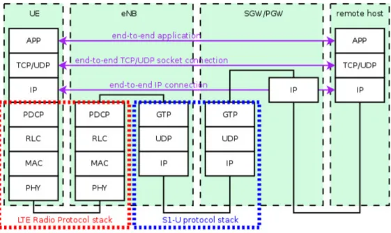
Figure 3.3 LTE-EPC data plane protocol stack. . . 13
Figure 3.4 LTE protocol architecture (downlink) [1]. . . 14
Figure 3.5 LTE physical layer blocks. . . 14
Figure 3.6 LTE OFDM modulation. . . 15
Figure 3.7 Structure of cell-specific reference signal within a pair of resource blocks. 15 Figure 3.8 OFDM modulation by IFFT processing. . . 16
Figure 3.9 Overview of Turbo decoding. . . 18
Figure 3.10 Block diagram of a MIMO-BICM system. . . 19
Figure 3.11 Decoding tree of the FSD algorithm for a 4 × 4 MIMO system with QPSK symbols. . . 19
Figure 3.12 Handle the workload for N codewords by partitioning of threads. . . 20
Figure 3.13 CUDA Memory Model. . . 22
Figure 3.14 Dual Channel DDR Memory. . . 25
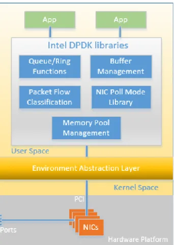
Figure 3.15 Intel Data plane development kit (DPDK) architecture. . . 27
Figure 3.16 EAL initialization in a Linux application environment. . . 28
Figure 4.1 FFT factorization of DFT for N = 8. . . 32
Figure 5.1 Computation time of matrix multiplication vs the matrix size for GPU (Geforce GTX 660 Ti)(with and without shared memory) and multi-core (8-multi-core CPU x86 64). GPU Clock rate and CPU Clock rate are about 1 GHz and 3 GHz, respectively. . . 42 Figure 5.2 One step of a summation reduction based on the first approach :
Assuming 8 entries in cache variable, the variable i is 4. In this case, 4 threads are required to calculate the sum of the entries at the left side with the corresponding ones at the right side. . . 51 Figure 5.3 Tree-based summation reduction : Entries are combined together based
on a tree structure. . . 52 Figure 5.4 CPU/GPU times for (a) GPUArray method (b) gather method in
computation of FFT using Matlab implementation on GPU. . . 56 Figure 5.5 Speedup vs matrix size for Matlab based computation of matrix
inversion on GPUs : (a) including the times of data transfer from RAM to GPU memory and calculation of matrix inverse on GPU (b) including the times of data transfer to and from GPU memory and calculation of matrix inverse on GPU. . . 58 Figure 5.6 Speedup vs matrix size for Matlab based computation of matrix
addition on GPUs : (a) including the times of data transfer from RAM to GPU memory and calculation of matrix addition on GPU (b) including the times of data transfer to and from GPU memory and calculation of matrix addition on GPU. . . 60 Figure 5.7 Speedup vs matrix size for Matlab based computation of matrix
multiplication (Y = A · X) on GPUs : (a) including the times of data transfer from RAM to GPU memory and calculation of matrix multiplication on GPU (b) including the times of data transfer to and from GPU memory and calculation of matrix multiplication on GPU. . 61 Figure 6.1 Architecture of a data center. . . 64 Figure 6.2 Computation times of FFT when running on slave core (a) MKL with
DPDK without core isolation (b) MKL with DPDK and core isolation (c) MKL without DPDK (d) straight C implementation. . . 69
Figure 6.3 Histograms of computation times running on slave core (a) MKL with DPDK without core isolation (b) MKL with DPDK and core isolation (c) MKL without DPDK (d) straight C implementation. . . 70
LIST OF ACRONYMS AND ABBREVIATIONS
3GPP 3rd Generation Partnership Project AM Acknowledged Mode
AS Access Stratum
DL Downlink
DPDK Data Plane Development Kit FE Full Expansion
FEC Forward Error Correction
FPFSD Fixed-complexity sphere decoder GPU Graphics processing unit
LLRs Log-likelihood ratios LTE Long Term Evolution MAC Media Access Control
MIMO Multiple Input Multiple Output MKL Math Kernel Library
MPI Message Passing Interface SDR Software Defined Radio
NMM Network-Integrated Multimedia Middleware PDCP Packet Data Convergence Protocol
PDU Protocol Data Unit PHY Physical layer RLC Radio Link Control RRC Radio Resource Control SDU Service Data Unit SE Single-path search SNR Signal to Noise Ratio
SSFE Selective spanning with fast enumeration TM Transparent Mode
UE User Equipment
UM Unacknowledged Mode
CHAPTER 1
INTRODUCTION
Recent advances in information and communication technology have drawn attention from the telecommunication industry to more efficient implementation of wireless standards. Specifically, a great deal of attention is dedicated to develop a form of Software Defined Radio (SDR) that performs different signal processing tasks over the telecommunication cloud [2]. However, performing the needed complex operations involved in the modern cellular technologies and meeting the real time constrains impose needs for extra computational resources, which may not be available in current telecommunication infrastructure.
The most recently deployed cellular technology, the Long-Term Evolution (LTE) standard, is an example of such complex systems. Real time and low latency computations are critical aspects in cloud-based implementation of LTE, which involves many challenges in practice. Specifically, the design and implementation of real-time and low-latency wireless systems aims at achieving two goals : first reducing the latency by recognizing its time consuming parts ; second proposing solutions to reduce the variability (randomness) in the processing times. In this thesis, we address the following objectives :
1. identifying computational bottlenecks in the LTE ;
2. reducing the computational latency to increase performance ;
3. implementing (near) real-time processing algorithms by reducing variability of computation times ;
4. studying the computational performance of different modules of LTE when implemented on graphics processing units ;
5. studying the computational performance of LTE modules for implementation on central processing units using different implementation tools.
Academia and industry have shown interest in using Graphics Processing Units (GPUs) for accelerated implementation of different applications. Essentially, GPUs are widely used for accelerating computation times because they are offering large number of processing cores and high memory bandwidth. For instance, Geforce GTX 660 Ti offers 7 multi-processors and 192 independent cores for each multi-processor. That is very promising and suggests possible accelerations of 1000 times using GPU implementation. In spite of such large number of
available processing elements, we could never get acceleration larger than 10 and in many case we got no acceleration at all. That is why we looked at other acceleration methods to verify the efficiency. Moreover, Intel has also provided a Data Plane Development Kit (DPDK) [3] and a Math Kernel Library (MKL) [4] for low latency processing of telecommunication tasks over more conventional central processing units.
1.1 Contributions
In this thesis, we study different parts of the LTE standard and identify the time consuming portion which may act as computational bottlenecks in an implementation. Then, we propose different solutions for parallel computing of those computational bottlenecks and discuss their performance. Specifically, we study the implementation of different matrix and vector operations over graphical processing units and central processing units. For each case, we propose different implementation approaches and evaluate their efficiency by comparing their computation times. We use the fast Fourier transform (FFT) as a benchmark for many of our analysis as it is found to be one of the largest computational burdens for LTE. As it was discussed earlier, our primary goal is to achieve near-deterministic and low latency processing times for LTE operations.
This thesis focus on studying different means of performing some complex parts of LTE (specifically the FFT) and its main contributions can be summarized as follows :
– implementation of FFT, convolution, matrix multiplication and inversion using CUDA on GPUs,
– implementation of FFT, matrix multiplication and inversion using MATLAB on GPUs, – analysis of related results and suitability of CPUs for supporting LTE tasks,
– implementation of FFT using Intel MKL on CPUs,
– implementation of FFT using DPDK and MKL on CPUs with and without the aid of isolation of processing units,
– comprehensive analysis of FFT implementation on CPUs in different scenarios.
1.2 Organization
This thesis is organized as follows. In Chapter 2, we present a comprehensive review of the literature on parallel processing. Further, we review the related literature about DPDK as a solution for parallel processing potentially useful in this thesis. In Chapter 3, we
provide a review of the LTE standard, discussing its different layers and its main functions. Specifically, we describe the structure of orthogonal frequency division multiplexing (OFDM) using FFT and inverse FFT operations. Turbo decoding and MIMO (multiple input and multiple output) detection mechanisms are also described in Chapter 3. Further, we describe the GPU programming model for parallel programming. Chapter 3 concludes by introducing MKL and DPDK.
In Chapter 4, we discuss different algorithms for implementation of FFT (including Cooley-Tukey and Stockham algorithms), matrix inversion, convolution and cross-correlation. These algorithms are used in the following chapters for implementation on the hardware devices.
In Chapter 5, we describe parallel implementations of different operations on GPUs. We use MATLAB and CUDA for implementation of dense matrix multiplication, FFT, matrix inversion, convolution and addition. Our experimental results for implementation of these operations on GPUs are also presented in this chapter.
Although GPUs include large number of cores and computation elements, we could not get high percentage of acceleration using them. For that reason, in Chapter 6, we study the feasibility of using DPDK and MKL to achieve near deterministic computation for LTE processes. Our experimental results show different performance in terms of the mean and variance of the computation times when DPDK and MKL libraries are used for isolation of the central processing unit. Our concluding remarks and future directions are presented in Chapter 7.
CHAPTER 2
LITERATURE REVIEW
LTE supports and takes advantage of a new modulation technology based on Orthogonal Frequency Division Multiplexing (OFDM) and Multiple Input Multiple Output (MIMO) data transmission. The benefits of LTE come from increased data rates, improved spectrum efficiency obtained by spatially multiplexing multiple data streams [5], improved coverage, and reduced latency, which makes it efficient for current wireless telecommunication systems. Since MIMO systems increase the complexity of the receiver module, high-throughput practical implementations that are also scalable with the system size are necessary. To reach these goals, we explore two solutions to overcome LTE computation latency, which are parallel processing using GPU and DPDK.
2.1 Parallel processing to reduce computation time of LTE
GPUs have been recently used to develop reconfigurable software-defined-radio platforms [6, 7], high-throughput MIMO detectors [8, 9], and fast low-density parity-check decoders [10]. Although multicore central processing unit (CPU) implementations could also replace traditional use of digital signal processors and field-programmable gate arrays (FPGAs), this option would interfere with the execution of the tasks assigned to the CPU of the computer, possibly causing speed decrease. Since GPUs are more rarely used than CPUs in conventional applications, their use as coprocessors in signal-processing systems needs to be explored. Therefore, systems formed by a multicore computer with one or more GPUs are interesting in this context. In [11], the authors implement signal processing algorithms suitable with parallel processing properties of GPUs to decrease computation time of multiple-input–multiple-output (MIMO) systems. They develop a novel channel matrix preprocessing stage for MIMO systems which is efficiently matched with the multicore architecture.
Work is needed to decrease the run time for those configurations not attaining real-time performance. The use of either more powerful GPUs or more than one GPU in heterogeneous systems may be promising solutions for this purpose. Another interesting
topic for research is to analyze the amount of energy consumed by the proposed GPU implementations. According to [11], channel Matrix preprocessing is well matched with GPU architectures and it reduces the order of computational complexity. According to [12], distributed Multimedia Middleware transparently combines processing components using CPUs, as well as local and remote GPUs for distributed processing. This middleware uses zero-copy to choose the best possible mechanism for exchanging data.
In [13], an effective and flexible N-way MIMO detector is implemented on GPU, two important techniques are used (instead of Maximum likelihood detection) : depth-first algorithms such as depth-first sphere detection and breadth-first algorithms such as the K-best. In depth-first sphere detection algorithm, the number of tree nodes visited vary with the signal to noise ratio (SNR). The K-best detection algorithm has a fixed throughput because it searches a fixed number of tree nodes independent of SNR. Compared to ASIC and FPGA, this implementation is attractive since it can support a wide range of parameters such as modulation order and MIMO configuration. In the second technique, selective spanning with fast enumeration (SSFE) and different permuted antenna-detection order are used in order to be well suited for GPUs. Moreover, modified Gram-Schmidt Orthogonalization to perform QR decomposition is implemented. This implementation performs MIMO detection on many subcarriers in parallel using hundreds of independent thread-blocks to achieve high performance by dividing the available bandwidth into many orthogonal independent subcarriers.
In [14], a 2 × 2 MIMO system using a GPU cluster as the modem processor of an SDR system is implemented for the purpose of exploiting additional parallel processing capabilities over a single GPU system. Moreover, a 3-node GPU cluster using MPI-based distributed signal processing is applied to some modules that need relatively large amounts of computational capacity such as the frame synchronization module, the MIMO decoder, and the Forward Error Correction (FEC) decoder (Viterbi algorithm). It is only applied to WiMAX data. However, the clustered MPI-based signal processing efficiency achieved in the WiMAX system would be applicable to LTE systems. In [14], a Software Defined Radio Base Station (SDR BS) is implemented using two-level parallelism. One level of parallelism is obtained by the distributed processing provided by MPI and the other level of parallelism is the parallel processing performed at each node using a GPU.
Based on [15], it can be concluded that matrix inversion is a bottleneck if MMSE-based MIMO detectors were to be implemented on GPUs. In [15], each matrix of size N × N is mapped to N threads. In this approach, each thread reads N elements in a single matrix
from the shared memory, and N threads process a matrix inversion in parallel. In addition, multiple matrices can be inverted simultaneously in a block. Finally in a grid which is composed of several blocks, many matrices are processed, thus speeding up the algorithm. In this paper, two kinds of data transfers (synchronous and asynchronous) are considered. In the synchronous model, the kernel is executed after the data has been transferred completely. This paper mentions that frame synchronization, MIMO decoding, and Forward Error Correction (FEC) decoding are the most time consuming tasks of LTE. Another time consuming part of frame synchronization is cross-correlation. Frame synchronization on GPU has not been implemented yet. This work applied clustered MPI-based signal processing to WiMAX not to LTE.
The authors in [15] present an MMSE-based MIMO detector on GPU. Optimization strategies have been proposed to compute channel matrix inversion, which is the heaviest computational load in the MMSE detector. A Gaussian elimination approach with complete pivoting is employed to compute the matrix inversion. In [16] the authors mention that to improve coverage and increase data rate, LTE requires a very short latency of less than 1 millisecond across the backhaul network.
The authors in [17] explain that the high data rates of LTE enable interactive multimedia applications over networks. They investigated the performance of 2D and 3D video transmission over LTE by combining bandwidth scalability and admission control strategies in LTE networks.
In [18], the authors argue that minimizing the system and User Equipment (UE) complexities are the main challenges of LTE. It allows flexible spectrum deployment in LTE frequency spectrum as well as enabling co-existence with other 3GPP Radio Access Technologies (RATs). Also, they mention that load imbalance reduces LTE network performance because of non-uniform user deployment distribution. Load balancing techniques are proposed in this paper to improve network performance.
The authors in [8] develop a 3GPP LTE compliant turbo decoder accelerator on GPU. The challenge of implementing a turbo decoder is finding an efficient mapping of the decoder algorithm on GPU, e.g. finding a good way to parallelize workload across cores that allocates and uses fast on-die memory to improve throughput. This paper increases throughput through 1) distributing the decoding workload for a codeword across multiple cores, 2) decoding multiple codewords simultaneously to increase concurrency and 3) employing memory optimization techniques to reduce memory bandwidth requirements. In
addition, it also analyzes how different MAP algorithm approximations affect both throughput and bit error rate (BER) performance of decoders.
For simulation, the host computer first generates random 3GPP LTE Turbo codewords. After BPSK modulation, input symbols are passed through the channel with additive white Gaussian noise (AWGN), the host generates LLR values based on the received symbols which are fed into the Turbo decoder kernel running on a GPU.
2.1.1 Summary
As this study shows, the LTE challenges are : 1) a latency requirements of less than 1ms [16], 2) minimizing the system and User Equipment (UE) complexities, 3) allowing flexible spectrum deployment, 4) increasing capacity, 5) improving QoS, 6) enabling co-existence with other 3GPP Radio Access Technologies (RATs) [18], 7) scalability [17], and load balancing [18]. Since, implementation of LTE functions in data centers requires computing resources in wireless networks, it leads to more advanced algorithms and signal processing as well as load balancing and multi-threading.
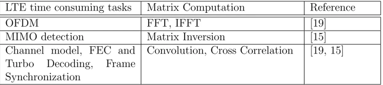
Centralized radio access network needs to leverage massive parallel computing in order to increase data rate and decrease latency. Table 2.1 summarizes reported analysis and means of dealing with LTE time consuming tasks, which include FFT/IFFT in OFDM [19], matrix inversion in MIMO detection [15], convolution and cross correlation in channel model [19, 15].
Table 2.1 LTE time consuming tasks.
LTE time consuming tasks Matrix Computation Reference
OFDM FFT, IFFT [19]
MIMO detection Matrix Inversion [15]
Channel model, FEC and Turbo Decoding, Frame Synchronization
2.2 Reducing computation time of LTE using DPDK
All literature on DPDK that was found, relates to packet forwarding in layers two and three (L2 and L3). There is nothing related to computation and mathematical functions. In [20], the authors apply a combination of programmable hardware, general purpose processors, and Digital Signal Processors (DSPs) into a single die to improve the cost/performance trade off. Authors in [21] suggest to use Cloud infrastructure Radio Access Network (C-RAN) in two kinds of centralization (full and partial) to provide energy efficient wireless networks. The major disadvantage of this architecture is the high bandwidth and low latency requirements between the data center and the remote radio heads. Authors in [2] and [22] mention that SDN requires specific levels of programmability in the data plane and the Intel DPDK is a promising approach to improve performance in cloud computing applications. DPDK is proposed to enhance operating systems running on General Purpose Processors (GPPs) that already have some real-time capability.
Based on [2] DPDK proposes high performance packet processing. The authors in this paper propose Open flow 1.3 to implement the data plane. The authors also mention that the packet I/O overhead, buffering to DRAM, interrupt handling, memory copy and the overhead of kernel structures cause extra costs and delays, while using DPDK overcomes these bottlenecks. DPDK allows efficient transfer of packets between the I/O card and the code running in the user space. Transferring packets directly to L3 cache prevents to use high latency DRAMs. Thus DPDK increases performance.
2.3 Summary on literature review
The literature has shown ways to accelerate LTE with GPUs. It was reported that FFT/IFFT is the main time consuming function of OFDM and matrix inversion is a time consuming task associated with MIMO detection which can be possibly accelerated by GPU parallel processing. In fact the size of matrices for matrix inversion in LTE is small. By contrast, GPUs are more efficient for processing large number of data elements organized in a regular structure. Moreover, DPDK has a high performance packet processing capability. It helps implementing demanding applications on general purpose operating systems which have real-time capabilities.
CHAPTER 3
OVERVIEW OF LTE, GPU, DPDK
In this chapter we explain what is LTE. We describe layers of LTE and their main functionalities supported by the physical-layer processing blocks. As the main blocks of LTE in physical layer, we present OFDM and its implementation using FFT and IFFT. Also, we describe the Turbo decoder and MIMO detection. Since, GPUs are presented as a solution to reduce LTE latency, we describe the GPU programming model, and Geforce GTX 660 Ti specifications. MKL and DPDK features and usage are described as another solution to decrease latency.
3.1 LTE overview
Long term evolution (LTE) is based on the 3GPP standard that provides a downlink speed of up to 100 Mbps and an uplink speed of up to 50 Mbps. LTE brings many technical benefits to cellular networks. Bandwidth is scalable from 1.25 MHz to 20 MHz. This can suit the needs of different network operators that have different bandwidth allocations, and also allows operators to provide different services based on spectrum. LTE is also expected to improve spectral efficiency in 3G networks, allowing carriers to provide more data and voice services over a given bandwidth [1].
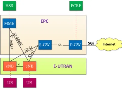
The LTE system architecture is based on the classical open system interconnect layer decomposition as shown in Fig. 3.3 (taken from [24]). Fig. 3.1 (taken from [23]) shows a high-level view of the LTE architecture. E-UTRAN (Evolved Universal Terrestrial Radio Access Network) and EPC (Evolved Packet Core) are two main components of LTE systems [23]. E-UTRAN is responsible for management of radio access and provides user and control plane support to the User Equipments (UEs). The user plane refers to a group of protocols used to support user data transmission, while control plane refers to a group of protocols to control user data transmission and managing the connection between the UE and networks such as handover, service establishment, resource control, etc. The E-UTRAN consists of only eNodeBs (eNBs) which provide user plane (PDCP/RLC/MAC/PHY) and control plane (RRC) protocol terminations toward the user equipment (UE). The eNBs are interconnected
with each other by means of the X2 interface. The eNBs are also connected by means of the S1 interface to the Evolved Packet Core (EPC), more specifically to the Mobility Management Entity (MME) by means of the S1-MME interface and to the Serving Gateway (SGW) by means of the S1-U interface.
EPC is a mobile core network and its main responsibilities include mobility management, policy management and security. The EPC consists of the Mobility Management Entity (MME), the Serving Gateway (S-GW), and the Packet Data Network Gateway (P-GW). The MME is the control node for the LTE access network. It is responsible for user authentication and idle mode User Equipment (UE) paging and tagging procedure including retransmissions. The functions of the S-GW is to establish bearers based on the directives of the MME. The PGW provides Packet Data Network connectivity to E-UTRAN capable UEs using E-UTRAN only over the S5 interface. Both E-UTRAN and EPC are responsible for the quality-of-service (QoS) control in LTE. The x2 interface provides communication among eNBs including handover information, measurement and interface coordination reports, load measurements, eNB configuration setups and forwarding of user data. S1 interface connects the eNBs to the EPC. The interface between eNB and S-GW is called S1-U and is used to transfer user data. The interface between eNB and MME is called S1-MME and is used to transfer control-plane information including mobility support, paging data service management, location services and network management. Home Subscriber Server (HSS) and the Policy Control and Charging Rules Functions (PCRF) are considered to be parts of the LTE core network [23].
PCRF UE UE S-GW S5 P-GW MME eNB eNB S1-U S1-U S1 -M M E S1 -M M E SGi Internet EPC HSS X2 E-UTRAN
Fig. 3.2 (taken from [24]) shows a diagram of the E-UTRAN Protocol Stack. Physical Layer carries all information from the MAC transport channels over the air interface. It takes care of link adaptation (AMC), power control, cell search (for initial synchronization and handover purposes) and other measurements (inside the LTE system and between systems) for the RRC layer. The Media Access Control (MAC) layer is responsible for mapping logical channels to transport channels. Also, it is resposible of Multiplexing the MAC SDUs from one or different logical channels onto transport blocks (TBs) to be delivered to the physical layer on transport channels. Demultiplexing of MAC SDUs from one or different logical channels from transport blocks (TBs) delivered from the physical layer on transport channels is another tasks performed by the MAC. Moreover, it schedules information reporting, corrects error through HARQ, handles priority between UEs by means of dynamic scheduling and between logical channels of one UE. The Radio Link Control (RLC) layer operates in 3 modes of operation : Transparent Mode (TM), Unacknowledged Mode (UM)1, and Acknowledged Mode (AM)2. It is responsible for
transfer of upper layer PDUs3, error correction through ARQ (only for AM data transfer),
concatenation, segmentation and reassembly of RLC SDUs4 (only for UM and AM data
transfer). RLC is also responsible for re-segmentation of RLC data PDUs (only for AM data transfer), reordering of RLC data PDUs (only for UM and AM data transfer), duplicate detection (only for UM and AM data transfer), RLC SDU discard (only for UM and AM data transfer), RLC re-establishment, and protocol error detection (only for AM data transfer). The main services and functions of the Radio Resource Control (RRC) sublayer include broadcast of System Information related to the non-access stratum (NAS)5, broadcast of System Information related to the access stratum (AS)6, paging7,
establishment, maintenance and release of an RRC connection between the UE and E-UTRAN, Security functions including key management, establishment, configuration, maintenance and release of point to point Radio Bearers. NAS protocols support the mobility of the UE and the session management procedures to establish and maintain IP connectivity between the UE and a PDN GW [24].
1. It does not require any reception response from the other party. 2. It requires ACK/NACK from the other party.
3. Protocol Data Unit (PDU) is information that is delivered as a unit among peer entities of a network and that may contain control information, such as address information, or user data.
4. Packets received by a layer are called Service Data Unit (SDU) while the packet output of a layer is referred to by Protocol Data Unit (PDU).
5. NAS is a functional layer in LTE stacks between the core network and user equipment. This layer is used to manage the establishment of communication sessions and for maintaining continuous communications with the user equipment as it moves.
6. AS is a functional layer in LTE protocol stacks between radio network and user equipment. It is responsible for transporting data over the wireless connection and managing radio resources.
Physical Layer (PHY) Media Access Control
(MAC) Radio Link Control
(RLC)
Radio Resource Control (RRC) Physical Channels Transport Channels Logical Channels
C
o
n
tr
o
l a
n
d
M
e
as
u
re
m
e
n
ts
Layer 2
Layer 3
Layer 1
Figure 3.2 Dynamic nature of the LTE Radio.
3.1.1 Layers of LTE and their main functionalities
Fig. 3.3 (taken from [24]) illustrates how the decomposition was done. The authors in [1] describe LTE layers in more details.
Packet Data Convergence Protocol (PDCP) performs IP header compression to minimize the number of bits to send over the radio channel. This compression is based on Robust Header Compression (ROHC). PDCP is also responsible for ciphering and for the control plane, integrity protection of the transmitted data, as well as in-sequence delivery and duplicate removal for handover. At the receiver side, PDCP performs deciphering and decompression operations.
Radio Link Control (RLC) performs segmentation/concatenation, retransmission handling, duplicate detection, and in-sequence delivery to higher layers. The RLC provides services to the PDCP in the form of radio bearers.
Media Access Control (MAC) is responsible for multiplexing of logical channels, hybrid-ARQ retransmission, and uplink and downlink scheduling. The scheduling functionality is located in the eNodeB for both uplink and downlink. The hybrid-ARQ protocol is applied to both transmitting and receiving ends of the MAC protocol. The MAC provides services to the RLC in the form of logical channels.
Figure 3.3 LTE-EPC data plane protocol stack.
multi-antenna mapping, and other typical physical-layer functions. The physical layer offers services to the MAC layer in the form of transport channels. Fig. 3.4 (taken from [1]) and Fig. 3.5 illustrate these functionalities graphically. In this figure, in an antenna and resource mapping block related to the physical layer, the antenna mapping module maps the output of the DFT precoder to antenna ports for subsequent mapping to the physical resource (the OFDM time-frequency module). Each resource block pair includes 14 OFDM symbols (one subframe) in time which follows in OFDM in LTE section.
3.1.2 OFDM in LTE
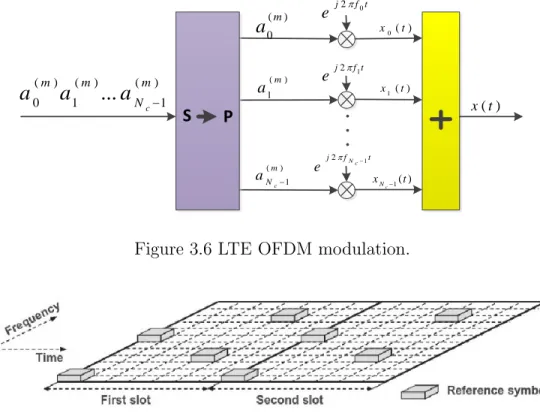
OFDM transmission is a kind of multi-carrier modulation. The basic characteristics of OFDM are : 1) the use of a very large number of narrowband subcarriers, 2) simple rectangular pulse shaping, and 3) tight frequency domain packing of the subcarriers with a subcarrier spacing 4f = 1/Tu. Where Tu is the per-subcarrier modulation symbol time. The subcarrier
spacing is thus equal to the per-subcarrier modulation rate 1/Tu. Fig. 3.6 (taken from [1])
illustrates a basic OFDM modulator. It consists of a bank of Nc complex modulators which
are transmitted in parallel, and each modulator corresponds to one OFDM subcarrier. Figure 3.7 (taken from [1]) illustrates the physical layer frame structure in a frequency-time grid. Time domain is divided into slots with duration of 0.5ms. Each sub-frame includes
Figure 3.4 LTE protocol architecture (downlink) [1].
Turbo
Encoding Scrambling Modulation FFT
IFFT Channel Estimation DFT Demodulation Turbo Decoding eNodeB Downlink Tx Chain
eNodeB Uplink Rx Chain
IQ Samples
IQ Samples
t f j c N e 2 1 t f j e 2 1 t f j e 2 0 ) ( 1 m Nc a ) ( 1 m a ) ( 0 m
a
) ( 1 t x c N ) ( 1 t x ) ( 0 t x P S ) ( 1 ) ( 1 ) ( 0...
m N m m ca
a
a
) ( t xFigure 3.6 LTE OFDM modulation.
Figure 3.7 Structure of cell-specific reference signal within a pair of resource blocks.
2 time slots. In fact, there are 2 × 7 symbols in each sub-frame and there are 10 sub-frames in each frame. Frequency domain consists of sub-carriers. Each sub-carrier spans 15 KHz. There are 12 sub-carriers in each sub-band. Thus, 12 sub-carriers are transmitted in each time slot. An OFDM signal x(t) during the time interval mTu ≤ t < (m + 1)Tu can be expressed
as : x(t) = Nc−1 X k=0 xk(t) = Nc−1 X k=0 a(m)k ej2πk4f t, (3.1)
where xk(t) is the kth modulated subcarrier with frequency fk = k 4 f and a (m)
k is the
complex modulation symbol applied to the kth subcarrier during the mth OFDM symbol
interval [1].
According to [1] the OFDM symbol consists of two major components : the CP and an FFT. As table 3.1 shows, LTE bandwidth varies from 1.25 MHz up to 20 MHz. In the case of 1.25 MHz transmission bandwidth, the FFT size is 128 and it is 2048 for 20MHz bandwidth.
Table 3.1 Transmission bandwidth vs. FFT size
Transmission bandwidth 1.25 MHz 2.5 MHz 5 MHz 10 MHz 15 MHz 20 MHz
FFT size 128 256 512 1024 1536 2048
3.1.3 OFDM implementation using FFT and IFFT
Fig. 3.6 illustrates, the basic principles of OFDM modulation. Choosing subcarrier spacing 4f equal to the per-subcarrier symbol rate 1/Tu, allows to implement an efficient FFT
processing. We assume sampling rate fs multiple of the subcarrier spacing 4f , fs = 1/Ts =
N 4f , the parameter N should be chosen to fulfill the sampling theorem [1]. The discrete-time OFDM signal can be expressed as :
xn= x(nTs) = N −1 X k=0 akej2πnk/N (3.2) where ak= ( a0k 0 ≤ k < Nc 0 Nc≤ k < N , (3.3)
Thus, the sequence xn is Inverse Discrete Fourier Transform (IDFT) of modulation symbols
a0, a1, ..., aNc−1 extended with zeros to length N to have a fixed length. As a result, OFDM modulation can be implemented by an IDFT of size N followed by digital to analog conversion which is shown in Fig. 3.8 [1].
1 c N a 1 a 0 a 1 N x 0 x P S 1 1 0a ...aNc a ) ( t x Size-N IDFT (IFFT) 0 0 P S 1 x D/A conversion
3.1.4 Turbo decoder
Turbo decoding as a forward error correction iterative algorithm achieves error performance near to the channel capacity. A Turbo decoder consists of two component decoders and two interleavers, which is shown in Fig. 3.9 (taken from [8]). It includes multiple passes through the two component decoders. One iteration includes one pass through both decoders. Despite the fact that both decoders perform the same sequence of computations, the decoders produce different log-likelihood ratios (LLRs). The de-interleaved LLRs of second decoder is the inputs of the first decoder and the interleaved LLRs of first decoder and channel are inputs of the second decoder. Each decoder operates a forward trellis traversal to decode a codeword with N information bits. Forward trellis traversal is used to compute N sets of forward state metrics, one α set per trellis stage. It is pursued by a backward trellis traversal which computes N sets of backward state metrics and one β set per trellis stage. Finally, the forward and the backward metrics are combined to compute the output LLRs [8]. Thus, turbo decoders, because of iterative decoding process and bidirectional recursive computing, requires optimal parallelism implementation to achieve high-data rates in telecommunication applications.
3.1.5 MIMO detection
Multiple-input multiple-output (MIMO) detection is the most time consuming task of LTE [15]. Authors in this paper proposed a novel strategy to implement the minimum mean square error for MIMO detection using OFDM. The key is using a massively parallel implementation of the scalable matrix inversion on graphics processing units (GPUs). A MIMO-OFDM system with M transmit antennae and N receive antennae can be expressed as
y = Hx + w (3.4)
where y = [y0, y1, y2, ..., yN −1]T is the N × 1 received data vector, H is the N × M MIMO
channel matrix, x is the M × 1 transmitted data vector and w is an M × 1 white Gaussian noise vector. MIMO detector estimate the transmitted data vector ˆx from the received noisy data y.
ˆ
Decoder 0 Decoder 1 1 Le+Lch La+Lch Le La Lc (Ys) Lc (Yp0) Lc (Yp1)
Figure 3.9 Overview of Turbo decoding.
Where MMSE minimize the mean square error of E{(ˆx − x)H(ˆx − x)} and E{.} is the expectation of random variable. GM M SE is
GM M SE = (HHH + IM/ρ)−1HH = J HH (3.6)
where ρ is the signal to noise ratio [15]. As a result, matrix inversion is the bottleneck of this algorithm.
3.2 A glance at literature review
In this section, we describe more about the contents of literature review. The goal is to demonstrate graphically what the authors did in the literature review and to provide some more descriptions.
3.2.1 MIMO detection
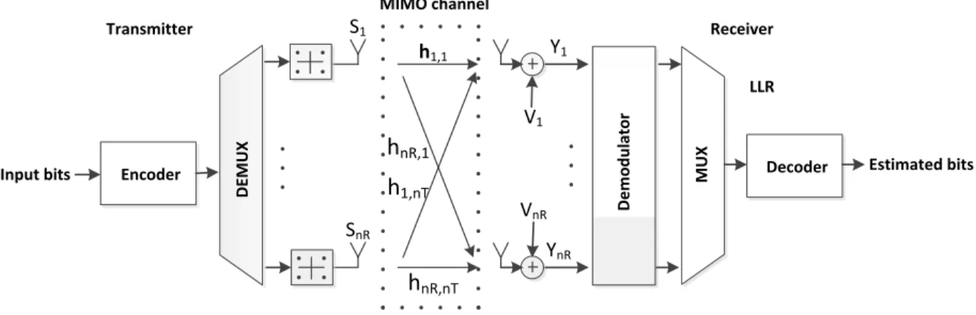
In the literature review chapter of 2, the authors report on how to implement MIMO on GPUs to decrease computation time by developing a novel channel matrix preprocessing stage that enables parallel processing. As Fig. 3.10 (taken from [11]) illustrates, MIMO with bit-interleaved coded modulation (BICM) is applied to implement a fully parallel soft-output fixed-complexity sphere decoder (FSD).
Fig. 3.10 and Fig. 3.11 (taken from [11]) depict how to compute parallel tree search and soft information about the code bits in terms of log-likelihood ratios (LLRs). They
h1,1 hnR,nT hnR,1 h1,nT V1 Y1 VnR YnR D e m o d u la to r M U X
Decoder Estimated bits LLR Receiver D EM U X Encoder Input bits Transmitter MIMO channel S1 SnR
Figure 3.10 Block diagram of a MIMO-BICM system.
also illustrate how a fully parallel fixed-complexity sphere decoder (FPFSD) method can be implemented. The norms of the columns of the channel matrix are obtained (requiring nT products, nT − 1 sums, and one squared root operation each) and sorted in ascending
order (n2
T floating point operations in the worst case). Thus, the complexity of this proposed
ordering is O(n2
T). This can be computed considerably faster if the norms are processed in
parallel. Generally, this ordering leads to more reliable decisions than random ordering, since symbols with the highest signal-to-noise ratio are detected before those with the lowest, thus reducing error propagation.
00
01 10 11
SE FE
Figure 3.11 Decoding tree of the FSD algorithm for a 4 × 4 MIMO system with QPSK symbols.
3.2.2 Turbo decoder
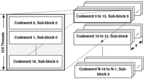
We discussed in literature review that authors in [25] applied turbo decoder on GPU. Their challenges were how to parallelize workload across cores. Fig. 3.12 (taken from [25]) shows how threads are partitioned to handle the workload for N codewords.
Figure 3.12 Handle the workload for N codewords by partitioning of threads.
The authors implemented a parallel Turbo decoder on GPU. As Fig. 3.12 depicts, instead of creating one thread-block per codeword to perform decoding, a codeword is split into P sub-blocks and decoded in parallel using multiple thread blocks. In this section, each thread-block has 128 threads and handles 16 codeword sub-thread-blocks [25].
3.3 GPU
Graphics Processing Units (GPUs) are a computing platform that has recently evolved toward more general purpose computations. This section describes the GPU programming model as viewed by the Nvidia company, which is based on the CUDA (Compute Unified Device Architecture) programming language and SIMD (Single Instruction, Multiple Data) architecture. the Geforce GTX 660 Ti will be used as an example as it was used in experiments.
3.3.1 GPU programming model
GPUs include a massive parallel architecture. They work best when supporting a stream programming model. Stream processing is the programming model used by standard graphics APIs. Stream processing is basically on-the-fly processing, i.e. data is processed as soon as it arrives. The results are sent as soon as they are ready. Thus, data and results are not stored in global (slow) memory to save memory bandwidth. We keep temporary data and results in local memory and registers. A stream is a set of data that require similar computations. Those similar computations execute as kernels in the programming model for GPUs. Since, GPUs can only process independent data elements, kernels are performed completely independently on the data elements of input streams to produce an output stream. Because GPUs are stream processors, processors can operate in parallel by running one kernel on many records in a stream at once. In CUDA, threads are assembled in blocks. Multiple thread-blocks are called a grid. A grid is organized as a 2D array of blocks, while each block is organized as 3D array of threads. At runtime, each grid is distributed over multiprocessors and executed independently [26].
Threads within a thread-block execute in blocks of 32 threads. When 32 threads share the same set of operations, they are assembled in what is called a warp and are processed in parallel in a SIMD fashion. If threads do not share the same instruction, the threads are executed serially [26]. Multiprocessor has control unit and it starts and stops threads on compute engines. Control unit can select which threads run as a warp. Control unit can schedule blocks on the compute engines. The number of threads is higher than the number of compute engines to allow multitasking to improve performance. When we do not have enough threads, we do not have a good occupancy. The occupancy is the time which takes to pass data through the slowest component in the communication path. If we choose proper number of threads per block, we balance processing time with the memory bandwidth.
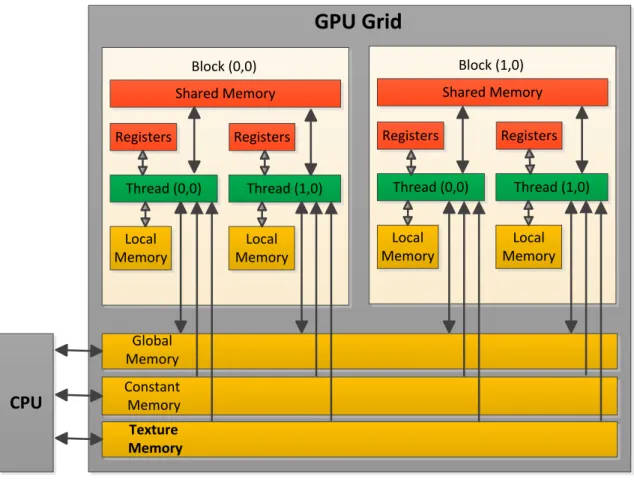
Fig. 3.13 (taken from [27]) illustrates CUDA memory model. As it shows, it consists of registers, local memory, shared memory, global memory, constant memory, and texture memory with the following descriptions.
Scalar variables that are declared in the scope of a kernel function and are not decorated with any attribute are stored in register memory by default. Access of register memory is very fast, but the number of registers that are available per block is limited. Any variable that can’t fit into the register space allowed for the kernel will spill-over into local memory. Shared memory increases computational throughput by keeping data on-chip. It must be declared
GPU Grid
Block (0,0) Shared Memory Registers Registers Thread (0,0) Thread (1,0) Local Memory Local Memory Global Memory Constant Memory Texture Memory Block (1,0) Shared Memory Registers Registers Thread (0,0) Thread (1,0) Local Memory Local MemoryCPU
Figure 3.13 CUDA Memory Model.
within the scope of the kernel function. When execution of kernel is finished, the shared memory in the kernel cannot be accessed. Global memory is declared outside of the scope of the kernel function. The access latency to global memory is very high (100 times slower than shared memory) but there is much more global memory than shared memory. Constant memory is used for data that will not change over the course of a kernel execution and it is cached on chip. Texture memory is read only has an L1 cache optimized for 2D spatial access pattern. In some situations it will provide higher effective bandwidth by reducing memory requests to off-chip DRAM. It is designed for graphics applications where memory access patterns exhibit a great deal of spatial locality [26].
3.3.2 Geforce GTX 660 Ti specifications
Geforce GTX 660 Ti GPU includes 7 multiprocessors, 192 CUDA cores per multiprocessor (compute capability), SIMDWidth (threads per warp) equals to 32, 2G bytes global memory, 1024 Max threads per block, (1024 × 1024 × 64) Max thread dimensions, (2G × 65536 × 65536) Max Grid dimensions and Clock rate is about 1GHz. The number of shared memory per multiprocessor is 49152 while the number of registers per multiprocessor is 65536 [27].
3.4 Intel Math Kernel Library (MKL)
Intel Math Kernel Library (MKL) is a highly optimized Math library. It uses for applications that require maximum performance. Intel MKL can be called from applications written in either C/C++, or in any other language that can reference a C interface. It includes 1) BLAS and LAPACK linear algebra libraries for vector, vector-matrix, and matrix-matrix operations, 2) ScaLAPACK distributed processing linear algebra libraries for Linux and Windows operating systems, as well as the Basic Linear Algebra Communications Subprograms (BLACS) and the Parallel Basic Linear Algebra Subprograms (PBLAS), 3) the PARDISO direct sparse solver, 4) FFT functions in 1D, 2D or 3D, 5) Vector Math Library (VML) routines for optimized mathematical operations on vectors, 6) Vector Statistical Library (VSL) routines, which offer high-performance vectorized random number generators (RNG) for several probability distributions, convolution and correlation routines, and summary statistics functions, 7) Data Fitting Library, which provides capabilities for spline-based approximation of functions, derivatives and integrals of functions, and search, and 8) Extended Eigen solver and a shared memory programming (SMP) version of an eigen solver. For details see the Intel MKL Reference Manual. In this thesis, MKL is used to compute FFT. The results are shown in Chapter 6. Algorithm 3.1 describes the implementation of FFT by MKL.
In this algorithm, lines 6 and 7 allocates the descriptor data structure and initializes it with default configuration values. Line 8 performs all initialization for the actual FFT computation. The DftiComputeForward function accepts the descriptor handle parameter and one or more data parameters. Given a successfully configured and committed descriptor, this function computes the forward FFT. Line 10 frees the memory allocated for a descriptor [28]. Note that we must add 3 libraries (mkl intel ilp64, mkl core and mkl sequential) for compilation.
Algorithm 3.1 Float Complex FFT using MKL[28]
1: #include ”mkl df ti.h”
2: f loat Complex x[N ];
3: DF T I DESCRIP T OR HAN DLE my desc1 handle;
4: M KL LON G status;
5: //...put input data into x[0], ..., x[N − 1];
6: status = Df tiCreateDescriptor
7: (&my desc1 handle, DF T I SIN GLE, DF T I COM P LEX, 1, N );
8: status = Df tiCommitDescriptor(my desc1 handle); 9: status = Df tiComputeF orward(my desc1 handle, x);
10: status = Df tiF reeDescriptor(&my desc1 handle);
11: / ∗ result is x[0], ..., x[N ] ∗ /
3.5 DPDK
DPDK is an optimized data plane software solution developed by Intel for its multi-core processors. It includes high performance packet processing software that combines application processing, control processing, data plane processing, and signal processing tasks onto a single platform. DPDK has a low level layer to improve performance. It has memory management functions, network interface support and libraries for packet classifications.
3.5.1 DPDK features
DPDK is a core application that includes optimized software libraries and Network Interface Card (NIC) drivers to improve packet processing performance by up to ten times on x86 platforms [3]. On the Hardware side, DPDK has the capabilities to support high speed pipelining, low latency transmission, exceptional QoS, determinism, Real time I/O switching. Intel Xeon series with an integrated DDR3 memory controller and an integrated PCI Express controller lead to lower memory latency.
DPDK features are : 1) It does some of the management tasks that are normally done by the operating system (it does those tasks with low overhead), 2) DPDK uses a run-to-completion model and a parallel computation model which runs one lcore followed by another lcore for next processing step, 3) DPDK uses Poll mode (i.e. it does not support interrupts) which is simpler than interrupts, thus it has lower overhead, 4) DPDK allocates memory from kernel at startup. 5) DPDK is pthread based but abstracts the pthread create, join, and provides a wrapper for the worker threads, and 6) DPDK supports Linux Multi-process.
As Fig. 3.14 (taken from [29]) illustrates, Dual Channel DDR memory uses two funnels (and thus two pipes) to feed data to the processor. Thus, it delivers twice the data of the single funnel. To prevent the funnel from being over-filled with data or to reverse the flow of data through the funnel, there is a traffic controller or memory controller that handles all data transfers involving the memory modules and the processor [29].
Figure 3.14 Dual Channel DDR Memory.
Thread is a procedure that runs independently from its main program. Pthread comes from IEEE POSIX 1003.1c standard. In fact it is Posix thread. It is one kind of thread. It is a software which a core executes. Pthread is light weight thread. Managing threads requires fewer system resources than managing processes. The most important functions of Pthread library are pthread create and pthread join. Pthread create is a function to create a new thread. Since, we need to manually terminate all threads before the main thread ends, pthread join does this task. When a parent thread (main thread) creates a child thread, it meets pthread join waits until the child thread’s execution finishes, and safely terminates the child thread.
Moreover, standard Linux operating system can also help to reduce overhead. In particular, using core affinity, disabling interrupts generated by packet I/O, using cache alignment, implementing huge pages to reduce translation look aside buffer (TLB) misses, prefetching, and new instructions save time.
On the computing side, DPDK includes dynamic resource sharing, workload migration, security, OpenAPIs, a developer community, virtualization and power management. Moreover, DPDK uses threads to perform zero-copy packet processing in parallel in order to reach high efficiency. Additionally, in its Buffer Manager, each core is provided a dedicated buffer cache to the memory pools which provides a fast and efficient method for quick access and release of buffers without lock. Fig. 3.15 illustrates Intel’s DPDK architecture. A
Buffer/Memory pool manager in DPDK provides NUMA (Non Uniform Memory Access) pools of objects in memory. Each pool utilizes the huge page table support of modern processors to decrease Translation Lookaside Buffer (TLB) misses and uses a ring (a circular buffer) to store free objects. The memory manager also guarantees that accesses to the objects are distributed across all memory channels. So, DPDK memory management includes NUMA awareness, alignment, and huge page table support which means that the CPU allocates RAM by large chunks. The chunks are pages. Less pages you have, less time it takes to find where the memory is mapped.
DPDK allows user applications to run without interrupts that would prevent deterministic processing. The queue manager uses lockless queues in order to allow different modules to process packets with no waiting times. Flow classification leverages the Intel Streaming SIMD Extensions (SSE) in order to improve efficiency. Also, Intel DPDK includes NIC Poll Mode drivers and libraries for 1 GbE and 10 GbE Ethernet controllers to work with no interrupts, which provides guaranteed performance in pipeline packet processing. DPDK’s Environment Abstraction Layer (EAL) contains the run-time libraries that support DPDK threads [30].
3.5.2 How to use DPDK
To install DPDK, it is important to have kernel version >= 2.6.33. The kernel version can be checked using the command of ”uname − r”. There is an installation guide for DPDK in [31]. To start using DPDK, in example directory of DPDK, there are sample codes such as helloworld and codes for packet forwarding L2 and L3. These codes are explained in [32]. Thus, it is important to know how to run helloworld file of DPDK. As it is in the DPDK documents in [31], to compile the application, you should go to your directory and configure two environmental variables of RT E SDK and RT E T ARGET before compiling the application. The following commands show how those two variables can be set :
cd examples/helloworld Set the path :
export RTE SDK=$HOME/DPDK Set the target :
export RTE TARGET=x86 64-default-linuxapp-gcc Build the application by :
make
Figure 3.15 Intel Data plane development kit (DPDK) architecture. ./build/hellowworld -c f -n 4
I used the following command to run my application (I put MKL FFT function, which I explained it MKL section, in helloworld file) :
./build/helloworld -c 5 -n 1 –no-huge
Where -c is COREMASK. It is an hexadecimal bit mask of the cores to run on. Core numbering can change between platforms and should be determined beforehand. You can monitor your PC cores by system monitor in linux.
-n NUM is number of memory channels per processor socket. and –no-huge means to use no huge page.
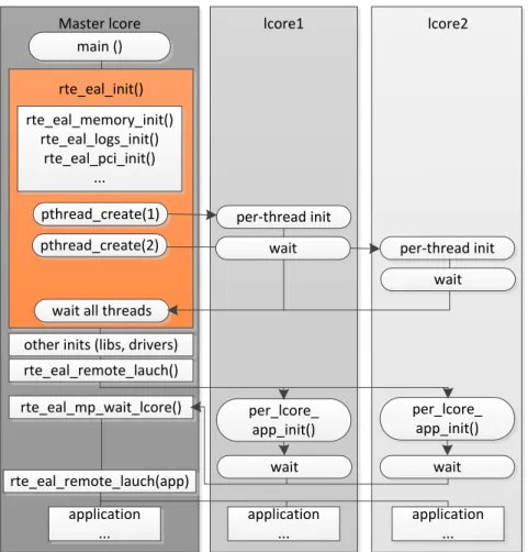
Based on DPDK documents, there are the list of options that can be given to the EAL : ./rte-app -c COREMASK -n NUM [-b <domain :bus :devid.func>] [–socket-mem=MB,...] [-m MB] [-r NUM] [-v] [–file-prefix] [–proc-type <primary|secondary|auto>] [–xen-dom0]. As Fig. 3.16 (taken from [33]) depicts, the first step to write a code using DPDK is to initialize the Environment Abstraction Layer (EAL). It creates worker threads and launch commands to main. This function is rte eal init() in the master lcore. Indeed, Master lcore runs the main function. This function is illustrated in algorithm 3.2. This algorithm finishes
Master lcore rte_eal_init() rte_eal_memory_init() rte_eal_logs_init() rte_eal_pci_init() ... main () pthread_create(1) pthread_create(2)
wait all threads other inits (libs, drivers) rte_eal_remote_lauch() rte_eal_mp_wait_lcore() rte_eal_remote_lauch(app) application ... lcore1 lcore2 per-thread init
wait per-thread init wait wait wait application ... application ... per_lcore_ app_init() per_lcore_ app_init()
Figure 3.16 EAL initialization in a Linux application environment. the initialization steps. Then, it is time to launch a function on an lcore.
An lcore is an abstract view of a core. It corresponds to either the full hardware core when hyper threading is not implemented, or it is hardware thread of a core that has hyper threading. In algorithm 3.3 and 3.4 lcore hello() is called on every available lcore and the code that launches the function on each lcore is demonstrated, respectively.
Algorithm 3.2 EAL Initialization [32]
1: int main(intargc, char ∗ ∗ argv)
2: {
3: ret = rte eal init(argc, argv);
4: if ret < 0 then
5: rte panic(”Can not init EAL”);
Algorithm 3.3 Definition of function to call lcore
1: static int lcore hello( attribute ((unused)) void ∗ arg)
2: {
3: unsigned lcore id;
4: lcore id = rte lcore id();
5: printf (”hello f rom core %u”, lcore id);
6: return 0;
7: }
Algorithm 3.4 Launch the function on each lcore
1: / ∗ call lcore hello() on every slave lcore ∗ / 2: RT E LCORE F OREACH SLAV E(lcore id)
3: {
4: rte eal remote launch(lcore hello, N U LL, lcore id);
5: }
6: / ∗ call it on master lcore too ∗ /
7: lcore hello(N U LL);
Those algorithms exist in Helloworld example. To explain it clearly, I divided that code to several parts. Then I put my FFT MKL function (in MKL section) in that code. Replace your function with lcore hello function. The function of lcore hello just write hello at the output. A function of rte eal remote launch() sends a message to each thread telling what function to run. Rte eal mp wait lcore() waits for thread functions to complete and rte lcore id() returns core id. Pthread create is a function to create a new thread. Wait all treads means to wait all threads finish their tasks. More explanations are in [32]. In chapter 6, we explain the usage of MKL and further discuss its advantages. To do isolcpus, modify grub file such as below (it depends on the operating system).
GRUB CMDLINE LINUX=”isolcpus = 4,5,6,7” in /etc/default/grub file. Perform grub-mkconfig -o /boot/grub/grub.cfg.
CHAPTER 4
FFT, MATRIX INVERSION AND CONVOLUTION ALGORITHMS
Since Fast Fourier Transform (FFT), matrix inversion and convolution are our benchmark in this thesis, the aim of this chapter is to describe in more details their algorithms in order to know if they have a potential for parallel implementation. We explain FFT and Discrete Fourier Transform (DFT) Radix-4. Then we perform radix-4 FFT using Matlab. Also, we present FFT Cooley-Tukey and Stockham algorithms to be familiar with different FFT algorithms. Finally, we show Gaussian Elimination algorithm for matrix inversion as well as introducing convolution and cross-correlation. We describe computational complexity order of all these functions. In the next chapter we will see how to accelerate the computation of these algorithms.
4.1 Fast Fourier Transform
This section describes DFT, that is, a Fourier transform as applied to a discrete complex valued series. For a continuous function of one variable x(t), the Fourier Transform X(f) is defined as :
X(f ) = Z ∞
−∞
x(t)e−j2πf tdt (4.1)
and the inverse transform as
x(t) = Z ∞
−∞
X(f )ej2πf tdf (4.2)
where j is the square root of −1. Consider a complex series x(k) with N samples x0, x1, x2, · · ·
, xN −1. Where x is a complex number. Further, assume that the series outside the range 0,
N − 1 is extended N -periodic. So that xk = xk+N for all k. The following equation represents
the DFT in matrix form with input vector x with dimension of N and output vector X[k] (see[34]). X[k] = N −1 X n=0 x[n]e−j2πnk/N (4.3)
where n ∈ [0; N − 1] and k ∈ [0; N − 1]. The sequence x[n] is referred to as the time domain and X[k] as the frequency domain. The DFT can be written in the matrix form as X = FNx
where FN is an N × N matrix given by
[FN]rs= wrs (4.4)
where
w = e−j2π/N. (4.5)
The inverse equation is given by :
x = 1 N F
∗
NX. (4.6)
Where ∗ means complex conjugate. Figure 4.1 (taken from [34]) illustrates FFT computation for N = 8 graphically. The output of this figure is the vector X in reverse bit order. As this figure shows, there is a potential to perform parallelism in this algorithm. In the next chapter, we show how to leverage parallelism to reduce computational time of FFT. For a value N = 2n, the FFT factorization includes log
2N = n iterations, each containing N/2
operations for a total of (N/2)log2N operations. This factorization is a base-2 factorization
applicable if N = 2n.
4.1.1 Discrete Fourier Transform Radix-4
In this section we show that how to compute Discrete Fourier Transform Radix-4 and how the computational load of radix-4 is lower. The sth sample of time series calculated by
sampling of f (t) in a duration T . DFT of N samples is derived by [35]
Fr = 1 N N −1 X s=0 ej2πrs/Nfs (4.7)
where Fr is the rth Fourier coefficient and j =
√
−1. We define TN as :
(TN)rs= ej2πrs/N (4.8)
x 0 x 1 x 2 x 3 x 4 x 5 x 6 x 7 X 7 X 3 X 5 X 1 X 6 X 2 X 4 X 0 + -+ -+ -+ -+ -+ -+ -+ -+ -+ -+ -+ -v0 v1 v2 v3 v4 v5 v6 v7 l7 l6 l5 l4 l3 l2 l1 l0 W 2 W 2 W 2 W 3 W 1 W 0 h0 h1 h2 h3 h7 g2 g1 g0 g7
Figure 4.1 FFT factorization of DFT for N = 8. where
w = ej2π/N (4.10)
Equation (4.7) can be written in the form of
F = (1/N )TNf. (4.11)
If N = rn, n is integer and r is basis, we can write TN = P (r) N T 0 N (4.12) TN0 = PN0(r)TN (4.13) and PN0(r) = {PN(r)}−1 (4.14)
Where PN(r) is a permutation matrix specific to the basis r. Thus Equation (4.12) expressed that we can show matrix TN based on its transpose matrix T
0
N using permutation matrix P (r) N .
Matrix TN0 is partitioned into r × r square sub-matrices with dimension of N/r × N/r. TN/r
is expressed in terms of TN/r2. This process is iteratively applied. The symbol × is Kronecker product of matrices. The ith iteration is represented as :
TN/k = PN/kr (TN/rk× Ir)D (r)
![Figure 3.4 LTE protocol architecture (downlink) [1].](https://thumb-eu.123doks.com/thumbv2/123doknet/2322818.29475/28.918.110.728.113.636/figure-lte-protocol-architecture-downlink.webp)