Phonon Transport Analysis of Thermal Conductivity in Particulate Nanocomposites

ARASH BEHRANG

D´EPARTEMENT DE G´ENIE CHIMIQUE ´

ECOLE POLYTECHNIQUE DE MONTR´EAL

M´EMOIRE PR´ESENT´E EN VUE DE L’OBTENTION DU DIPL ˆOME DE MAˆITRISE `ES SCIENCES APPLIQU´EES

(G´ENIE CHIMIQUE) AO ˆUT 2012

c

´

ECOLE POLYTECHNIQUE DE MONTR´EAL

Ce m´emoire intitul´e:

PHONON TRANSPORT ANALYSIS OF THERMAL CONDUCTIVITY IN PARTICULATE NANOCOMPOSITES

pr´esent´e par: BEHRANG Arash

en vue de l’obtention du diplˆome de: Maˆıtrise `es Sciences Appliqu´ees a ´et´e dˆument accept´e par le jury d’examen constitu´e de:

M. LEGROS Robert, Ph.D., pr´esident

M. LAFLEUR Pierre, Ph.D., membre et directeur de recherche M. GRMELA Miroslav, Ph.D., membre et codirecteur de recherche M. DUBOIS Charles, Ph.D., membre et codirecteur de recherche M. FAVIS Basil, Ph.D., membre

I dedicate this dissertation to my family. You are my life, my love and my reason for being. It is dedicated to my lovely wife, Sara with love. I am truly grateful for her immense love and patience throughout my graduate career. A special feeling of gratitude to my father and mother who have never left my side and supported me spiritually and materially since I was born.

Acknowledgement

First and foremost, I would like to express my unyielding gratitude to my supervisors, Professor Miroslav Grmela, Professor Charles Dubois and Professor Pierre Lafleur for their unselfish guidance, expertise, and friendship. They always took the time to guide me, to challenge me, and to help me develop my skills as a scientist and as a person.

Les mod`eles th´eoriques ont ´et´e pr´esent´es pour la pr´ediction de la conductivit´e thermique de composites constitu´es de particules sph´eriques. Parmi ces mod`eles, seuls quelques-uns d’entre eux sont en mesure de pr´edire correctement la conductivit´e thermique de nanocomposites. La difficult´e `a mod´eliser correctement cette propri´et´e physique origine de la diff´erence entre la conductivit´e de la matrice et des particules `a l’´etat pur par rapport `a leurs valeurs respectives dans le composite. En cons´equence, la r´esistance thermique `a l’interface entre la matrice et les particules devient une variable importante de la conductivit´e thermique des mat´eriaux nanocomposites. Dans ce projet, l’analyse de l’´echange des phonons thermiques dans les milieux h´etrog´enes est r´ealis´ee et une formule g´en´erale de la conductivit´e thermique effective de nanocomposites est pr´esent´ee.

Dans la premire ´etape du travail, le transport de phonons `a l’interface entre la matrice et des nanoparticules est ´etudi´e. Cette investigation vise pr´esenter la r´esistance thermique sous une nouvelle forme. Les deux types de transport de phonons sur l’interface particule-matrice, soient diffus et sp´eculaire, sont pris en compte dans le calcul de la conductivit´e thermique effective pour les nanocomposites particulaires.

Dans un deuxi`eme temps, le mod`ele propos´e est ´evalu´e en regard de r´esultats num´eriques et exp´erimentaux disponibles dans la litt´erature. Cette ´evaluation tend `a prouver que le mod`ele propos´e est capable de pr´edire la conductivit´e thermique effective pour un large ´eventail de fractions volumiques et de tailles de particules.

Abstract

Theoretical models have been presented for predicting the thermal conductivity of com-posites consisting of spherical particles. Among these models, only a few of them are able to predict the thermal conductivity of nanocomposites. This is because the matrix and particle thermal conductivities in nanocomposites are not equal to their bulk values due to increased interface scattering. The boundary scattering becomes important when the characteristic length of the media is smaller than the bulk mean free path of phonons. The thermal boundary resistance at the interface between matrix and suspended parti-cles is affected on the thermal conductivity of nanocomposites. In this work, the phonon viewpoint of heat transport in heterogeneous media is investigated and a general formula for the effective thermal conductivity of particulate nanocomposites is presented.

In the first step of this project, the phonon scattering at the interface between matrix and nanoparticles is investigated. This study aims to present the thermal boundary re-sistance in a new form. Both diffuse and specular types of scattering of phonons on the particle-matrix interface are taken into account in the derivation of the effective thermal conductivity for the particulate nanocomposites.

In the next step, the proposed model is evaluated with numerical and experimental results available in literature. This evaluation is done to prove that the proposed model is able to predict the effective thermal conductivity in a wide range of the volume fractions and particle sizes.

Dedication . . . iii

Acknowledgement . . . iv

R´esum´e . . . v

Abstract . . . vi

Table of Contents . . . vii

List of Tables . . . ix List of Figures . . . x Chapter 1 Introduction . . . 1 Chapter 2 Background . . . 4 2.1 Heat Transfer . . . 5 2.2 Phonons . . . 6 2.3 Phonon Dispersion . . . 7

2.3.1 The vibration of crystal with a mono-atomic basis . . . 8

2.3.2 First Brillouin zone . . . 9

2.3.3 The vibration of crystal with a diatomic basis . . . 10

2.4 Macro and micro heat conduction . . . 12

2.4.1 Mean Free Path . . . 13

2.4.2 Scattering mechanisms . . . 13

2.5 Boltzmann Transport Equation . . . 15

2.5.1 Fourier’s law . . . 16

2.5.2 Hyperbolic heat equation (Cattaneo equation) . . . 19

2.5.4 The equation of phonon radiative transfer (EPRT) . . . 24

2.6 Thermal boundary resistance . . . 27

2.6.1 Diffuse mismatch model . . . 28

2.6.2 Acoustic mismatch model . . . 29

2.7 Thermal conductivity of an inhomogeneous media using the generalized self consistent method . . . 33

Chapter 3 Details about the modeling process . . . 37

3.1 Effective Thermal conductivity of the matrix . . . 38

3.2 Effective thermal conductivity of the suspended particles . . . 42

3.3 Effective thermal conductivity of the thin films . . . 43

3.4 Generic formula for the thermal conductivity in particulate nanocomposites 47 3.4.1 Minnich-Chen formula . . . 48

3.4.2 Novel formula . . . 49

Chapter 4 Discussion . . . 50

Chapter 5 Conclusion . . . 58

5.1 Conclusion . . . 59

5.2 Recommendation for future works . . . 59

Table 2.1 : Heat transfer based on Knudsen number [11]. . . 13 Table 2.2 : thermal boundary resistance based on acoustic and diffuse mismatch

models. . . 33 Table 3.1 : Derived transmission lengths for different boundary resistances. . . 40 Table 4.1 : Material parameters used in calculations. . . 53

List of Figures

Figure 2.1 : Schematic illustration of heat transfer under diffuse and ballistic

regimes [2]. . . 6

Figure 2.2 : Ball-spring model for introducing of the speed of phonon propa-gation [10]. . . 8

Figure 2.3 : Mono-atomic vibration of an atom chain [9]. . . 9

Figure 2.4 : (a)Phonon dispersion curve of a one-dimensional mono-atomic lattice chain, (b)Group velocity of a one-dimensional mono-atomic lattice chain. . . 10

Figure 2.5 : A chain of two atoms with different masses linked by springs with different constants [9]. . . 11

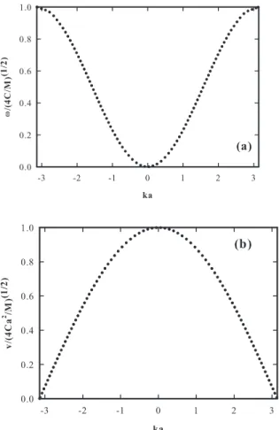
Figure 2.6 : (a)Phonon dispersion curve of a one-dimensional diatomic lattice chain, (b)Group velocity of a one-dimensional diatomic lattice chain. . . . 12

Figure 2.7 : Different phonon scattering mechanisms that reduce the thermal conductivity of the medium [14]. . . 14

Figure 2.8 : Thermal conductivity of CoSb3 as a function of temperature. The dots and solid lines represent the experimental and theoretical results [8]. . 15

Figure 2.9 : Schematic diagram qualitatively showing the temperature profiles under diffusive and ballistic phonon transport in steady sate condition [5]. 17 Figure 2.10 : Temperature profile at the steady state condition in macroscopic domain. . . 22

Figure 2.11 : Temperature profile at η = 10 in macroscopic domain. . . 23

Figure 2.12 : Temperature profile at η = 1 in macroscopic domain. . . 24

Figure 2.13 : Temperature profile at η = 1 for Kn = 1. . . 25

Figure 2.14 : Temperature profile at η = 1 for Kn = 10. . . 26

Figure 2.15 : Schematic of many possibilities of a phonon incident at the interface between two dissimilar materials [24]. . . 30

Figure 2.16 : Equilibrium and emitted phonon temperature at interface be-tween two dissimilar materials [4]. . . 32

Figure 4.1 : The totally specular and totally diffuse scaling factors plotted as a function of the volume fraction for various particle sizes. . . 51 Figure 4.2 : Interfacial specularity dependency of the thermal conductivity of

the matrix phase in different particle sizes when φ = 0.1. . . 52 Figure 4.3 : Interfacial specularity dependency of the thermal conductivity of

suspended particles in different particle sizes. . . 53 Figure 4.4 : Thermal conductivity of a SiGe nanocomposite as a function of

the particle diameter and the volume fraction. Proposed model is compared with Hashin’s model and obtained results from Monte Carlo simulations. . 54 Figure 4.5 : Thermal conductivity of a SiGe nanocomposite as a function of

the particle diameter and the volume fraction. Proposed model is compared with Hashin’s model, Nan’s model and obtained results from Monte Carlo simulations. . . 55 Figure 4.6 : Effective thermal conductivity of a SiGe nanocomposite comprising

spherical Si particles with the radius: (a) ap = 5nm, (b) ap = 25nm and

(c) ap = 100nm as a function of the particle volume fraction φ. . . 56

Figure 4.7 : Experimental and calculated values of the effective thermal con-ductivity as a function of the volume fractions φ of SiO2 and AlN

Chapter 1

Introduction

conduction cannot be directly applied. Furthermore, the heat transport becomes ballistic rather than diffusive. For the ballistic regime, temperature jumps occur at the boundaries of the media.

Boltzmann transport equation is the most commonly used method to study the heat trans-fer of the nanostructures. Various techniques have been developed to solve the Boltzmann transport equation in different geometries and conditions in order to provide more precise results.

Particle size and shape, volume fraction, orientation and the thermal conductance at the interface between two dissimilar materials are affected by the thermal conductivity of the inhomogeneous systems. For a heterogeneous media, such as nanocomposites and supperlattices, interfacial effects are very important. Phonon scattering at the interface forms a resistance against the motion of phonons and, consequently, decreases the phonon mean free path. This reduction in the phonon mean free path finally leads to a reduction in the effective thermal conductivity. While this term (i.e., interfacial effects ) would be neglected in macrostructures, when a heterogeneous media is under investigation, a better understanding of the behaviour of phonons at the interface between dissimilar materials is required. The interface can behave diffusely or specularly. Due to confinement of the phonon transport in the diffuse boundary scattering, the diffuse thermal conductivity is smaller than the specular thermal conductivity.

The main objective of this Master’s project is to introduce a new model to study the effective thermal conductivity of an inhomogeneous (suspended spherical particles in ma-trix) media by including the additional analysis details of the complex physics involved in the phonon scattering on the particle-matrix interface. To meet this goal, the following specific objectives have been considered:

(i). Modeling the thermal conductivity of composite using the generalized self-consistent method.

present a new term for the thermal boundary resistance.

(iii). Study the effects of particle size, volume fraction of particles, and specular prob-ability on the effective thermal conductivity of the nanocomposite and compare results with experimental data and previous numerical results.

In the scope of these specific objectives, by using the definition of the equilibrium thermal boundary resistance and the thermal conductivity based on the kinetic theory, the thermal boundary resistance is presented in the form of the mean free path. Then, both diffuse and specular types of phonon scattering on the particle-matrix interface are studied in the derivation of the totally diffuse, totally specular, and partially diffuse-partially specular thermal boundary resistance mean free paths. Finally, a generic model is introduced to study the thermal conductivity of the nanocomposite comprising spherical particles.

2.1

Heat Transfer

The energy transport process is a consequence of temperature difference known as heat transfer. Heat transfer phenomena are commonly seen in our everyday life and play a significant role in many industries and applications. Depending on the nature of the medium, three types of heat carriers are defined. Heat carriers convey heat from one side or arbitrary point to the other. Electrons, phonons, and photons are the most important heat carriers under different conditions. In a radiation mechanism, heat is carried by pho-tons while in conductors and semiconductors, heat is carried by electrons and phonons, respectively. According to the principle of quantum mechanics, both the wave and par-ticle natures of phonons would be studied in the heat transfer. The scattering among the phonons causes them to thermalize their energy and transfer heat from one point to another. Adequate scattering of the phonons establishes the local thermal equilibrium state where the temperature gradient can be defined [1, 2]. Although heat transfer is in-herently a non-equilibrium concept, the local thermal equilibrium is established where the deviation from equilibrium state is negligible. It is remarked that the classic irreversible thermodynamics (CIT) provides sufficient concepts to describe the equilibrium state. The classic irreversible thermodynamics breaks down under non-equilibrium conditions where basic physical quantities, such as temperature and mass, are not the only function of place (size and time dependency become effective) [3, 4]. In the macro-scale, the thermal conductivity coefficient is defined as a ratio between the heat flux (q) and the temperature gradient (∇T ) in the form of the well-known Fourier’s law.

Figure 2.1: Schematic illustration of heat transfer under diffuse and ballistic regimes [2].

By k, we denote the thermal conductivity of the media. Fourier’s law is a famous approach in the formulation of the macroscopic heat conduction, where the dependence of size and time on the heat transport is not important [5]. The diffuse collision (i.e., experiencing many collisions between phonons) and infinite heat propagation velocity are important features of the Fourier heat conduction. It is experimentally observed and physically supposed that even the smallest change in the temperature gradient is sensed after relaxation time. On the other hand, any temperature disturbance propagates at the finite velocity. In micro and nano-scales where time and size dependence are important, the validity of Fourier heat conduction is questioned. The qualitative behaviour of the thermal transport under diffuse and ballistic regimes has been illustrated in Figure (2.1).

2.2

Phonons

In crystalline solids, atoms are structured in periodical arrays known as lattice. Lattice vibrations contribute to thermal conductivity. In non-metal solids, heat is transferred by phonons. If two atoms in a solid body are far apart, an attractive force exists between the atoms, while the interaction force becomes repulsive (because of the overlap of electronic orbits in the atoms), if two atoms are close to each other. The minimum potential defines the equilibrium positions of the atoms where the repulsive and attractive forces balance each other. Atoms in a solid body vibrate about their equilibrium position. The vibration of each atom is constrained by its neighbouring atoms through the interatomic potential. A mass-spring system is a simplified picture of the interatomic interaction in crystalline solids. In such a system, the vibration of the atoms is not independent of each other and can cause the vibration of the whole system by creating a lattice wave in the system.

Clearly, the atoms near the hot side of the solid have larger vibrational amplitudes, which will be felt by atoms of the other side of the solid through the propagation and interaction of the lattice waves.

According to the principle of quantum mechanics, the energy of each lattice wave is dis-crete and must be a multiple of energy (hω), where h is the Planck’s constant and ω is the frequency. The minimum energy of hω, a quantized lattice wave, is called phonon. At a specific frequency and wavelength, phonon is a wave that travels through the entire crystal. Phonons can be considered as particles as long as they are much smaller than the crystal size. In this condition, the mass-spring picture of the crystal can be replaced by a box of phonon particles with random movement in the phase space.

Phonon dispersion curves are used to approximate how phonons are affected by the ther-mal conductivity of the media [4]. The phonon dispersion curves are usually divided into acoustic and optical branches. Low frequency acoustic phonon contributes significantly to thermal conductivity due to its large mean free paths. Although the optical phonon often does not contribute to heat transfer due to its small mean free path, it could be important when the characteristic length of the media is reduced [6–8].

2.3

Phonon Dispersion

The heat transfer in a solid is due to lattice vibration. This vibration is called thermal motion. Based on the lattice vibration theory, the atoms in a solid are close to each other, and interatomic forces keep them in position [9]. Vibration of the atoms takes place near their equilibrium positions. Understanding the interatomic forces enables us to further understand thermal properties of solids. If the bonds between two atoms are supposed to be stiff (such as, a rod), it will be impossible to determine the specific heat, thermal conductivity and melting point of the solid. Therefore, the elastic vibration model of the ball and spring should be considered (see Figure (2.2)). The spring is a conceptual representative of the repulsive and attractive forces [4, 10].

Figure 2.2: Ball-spring model for introducing of the speed of phonon propagation [10].

2.3.1

The vibration of crystal with a mono-atomic basis

It is assumed that the elastic response of crystal is a linear function of the force. So, Hook’s law could be used. According to this assumption, a harmonic vibration between atoms is considered, while anharmonic vibration is discussed at higher temperatures. Another assumption in the lattice vibration is that forces on an atom only come from its nearest-neighbours. A mono-atomic chain is illustrated in Figure (2.3). Allowing all atom masses (M) and spring constants (C) to be the same, the equation of motion of the atoms could be written as follows:

F = −C(us+1− us) − C(us− us−1) (2.2)

the equation of motion would be rearranged as follows:

Md

2_u s

dt2 = C(us+1− 2us+ us−1) (2.3)

The above equation is a special form of the differential wave equation

Md 2_u s dt2 = Ca 2d2us dx2 (2.4)

with a solution of the form us = u exp[−(iωt − kas)]. Where ω is the frequency of

Figure 2.3: Mono-atomic vibration of an atom chain [9].

Displacements at s ± 1 are

us±1 = u exp[−(iωt − ka(s ± 1))] (2.5)

Substituting the guessed expressions for us and us±1 into the equation (2.3) and after

some manipulations, the frequency of vibration in the mono-atomic chain is

ω = 2(r C M)| sin(

ak

2 )| (2.6)

2.3.2

First Brillouin zone

Only the wave-vectors, which are in the first Brillouin zone are physically affected by elastic waves. At the boundaries of the first Brillouin zone, the group velocity of phonons (vg ≡ ∂ω/∂k) is equal to zero, since the atoms at the boundaries oscillate in opposite

directions and their average movement tends to zero [9]. The first Brillouin zone takes place between −π/a < k < π/a. The group velocity in the first Brillioun zone is

vg = (

r Ca2

M ) cos( ak

Figure 2.4: (a)Phonon dispersion curve of a one-dimensional mono-atomic lattice chain, (b)Group velocity of a one-dimensional mono-atomic lattice chain.

Phonon dispersion and phonon group velocity curves for a 1-D mono-atomic lattice chain are illustrated in Figure (2.4). As previously explained and schematically illustrated in (2.4), the group velocity of phonons is equal to zero when phonons are at the boundaries of the first Brillouin zone.

2.3.3

The vibration of crystal with a diatomic basis

The relationship between the vibration frequency and the phonon wave-vector for a di-atomic chain follows the same procedure as the mono-di-atomic one. The interdi-atomic forces and the mass of the nearest-neighbour atoms are, however, not the same (Figure (2.5)). Equations of motion of the atoms are written as follows:

M1

d2_u s

Figure 2.5: A chain of two atoms with different masses linked by springs with different constants [9]. M2 d2_v s dt2 = −C2(us+1− vs) + C1(vs− us) (2.9)

Again, a wave form solution is guessed for the above equations. After some manipulations, we obtained the following equations:

(C1+ C2− M1ω2)u − (C1+ C2exp(iak))v = 0 (2.10)

(C1+ C2− M2ω2)v − (C1+ C2exp(iak))u = 0 (2.11)

The determinant must be zero,

2C1C2− (C1 + C2)(M1 + M2)ω2+ M1M2ω4− 2C1C2cos(ak) = 0 (2.12)

Solving the above equation, the phonon dispersion curve is represented for a diatomic chain. We use an example to introduce the phonon dispersion of a diatomic chain. Con-sider a linear diatomic chain in which the force constants are C1 = 10C and C2 = C with

masses M1 = 10M and M2 = M.

The result of the phonon dispersion curve when masses are not the same has been shown in Figure (2.6). Two branches are formed under this condition. The upper branch con-tains atoms, which oscillate out of phase. This branch is called the optical branch. The lower branch that corresponds to the in phase oscillation of atoms is called the acoustic branch [11]. The result of the group velocities of the acoustic and optical branches has been illustrated in Figure (2.6-b). The group velocity of the optical branch is significantly lower than the acoustic one. Note that the contribution of the optical branch in heat transfer can be neglected compared with the acoustic branch.

æ ææ æ æ ææ æ æ ææ æ æ æ 0.0 0.5 1.0 1.5 2.0 2.5 3.0 0 ka æ æ æ æ æ æ_{æ æ æ} æ æ_{æ æ} æ_æ æ_æ æ_æ æ æ æ æ æ æ æ æ æ æ æ æ æ æ æ æ æ æ æ æ æ æ æ æ æ æ æ æ æ æ æ ò ò ò ò ò ò ò ò ò_{ò ò ò ò ò ò} ò ò ò ò ò ò ò ò ò ò ò ò ò ò ò ò ò ò ò ò ò òò ò ò òò ò ò ò ò òò ò ò ò a) Acoustic branch b) Acoustic branch a b 0.0 0.5 1.0 1.5 2.0 2.5 3.0 0.00 0.05 0.10 0.15 0.20 0.25 ka v H Ca 2M L 1 2

Figure 2.6: (a)Phonon dispersion curve of a one-dimensional diatomic lattice chain, (b)Group velocity of a one-dimensional diatomic lattice chain.

2.4

Macro and micro heat conduction

In heat conduction two major areas are studied; macro-scale and micro-scale. The char-acteristic times and lengths are used to differentiate these regimes from each other. As previously discussed, the local thermal equilibrium is applied to study the heat conduction under macro-scale assumption where the heat transfer is independent of time and size. While time and size dependence of the heat transport is considered in the micro-scale formulation. The spatial and temporal dependence of the heat transport leads to the definition of several parameters that are used in the characterization of the micro-scale heat transfer [4, 5].

A famous dimensionless number which is widely used in the study of heat transfer is called the Knudsen number (Kn = Λ/L). When the mean free path (Λ) of the heat carriers

(i.e., phonons in our work) is much less than the characteristic length (L) of the system, the heat transport occurs in the macroscopic state and the regime behaves in a purely diffuse manner. In the opposite case, the microscopic heat transfer is established when the mean free path is larger than the characteristic length of the system. In this condition, the micro-scale heat transfer is categorized into partially ballistic (ballistic-diffusive) or purely ballistic heat transfer [12]. Heat transfer based on the Knudsen number has been tabulated in Table (2.1).

Table 2.1: Heat transfer based on Knudsen number [11]. Regime Method of calculation Knrange Continuum Navir-Stokes and energy equation 0.001 < Kn

with no slip/jump boundary condition

Slip flow Navir-Stokes and energy equation 0.001 < Kn < 0.1 with slip/jump boundary condition , DSMC

Transition BTE, DSMC 0 < Kn < 10 (Free Molecule) Kn >10

2.4.1

Mean Free Path

Fourier’s law is no longer valid when the characteristic length of the system is comparable or smaller than the mechanistic length, such as the mean free path. In order to better understand micro-scale heat transfer, the concept of the mean free path is described. The mean free path is the average distance covered by a moving particle (i.e., phonon in this work) between two subsequent collisions, which is affected by the direction and energy of the particle. The mean free path is usually used to estimate whether a phenomenon belongs to macro-scale regime or falls in the micro-scale regime [11, 13]. The chance of a successful collision between phonons decreases dramatically when the heat transfer regime falls into the micro-scale condition. On the other hand, the boundary scattering becomes significant and local thermal equilibrium is not valid unless it is at the boundaries [4].

2.4.2

Scattering mechanisms

The thermal conductivity of the media when Kn >> 1 decreases due to some scattering mechanism, which is not important in the corresponding bulk. Depending on the different types of scattering mechanisms, heat transfer is faced with different types of resistances shown in Figure (2.7). It is difficult to draw a conclusion about the relative strength of the scattering mechanisms on the thermal conductivity in the micro-scale media. It is

which creates resistance against heat flow and thus reduces the thermal conductivity of the media. It is noted that an infinite thermal conductivity is predicted, if the N-process is only taken into account [4, 11].

According to the Wien’s displacement law for phonons, the phonon wavelength

de-Figure 2.7: Different phonon scattering mechanisms that reduce the thermal conductivity of the medium [14].

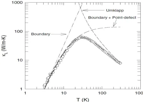
pends inversely on temperature. Therefore, the wavelength of the dominant phonons significantly decreases as the temperature rises. Figure (2.8) is a plot of the thermal conductivity of CoSb3 as a function of temperature. At low temperatures, the phonon

wavelength is long and the Umklapp scattering does not make a significant contribution to the thermal conductivity. As the temperature gradually increases, the phonon wave-length obviously decreases and becomes comparable to the size of the defects. Thus, defect scattering becomes important in moderate temperatures. Consequently, at high temperatures, the phonon wavelength is shortened and the Umklapp scattering becomes important [8, 11].

In order to study both micro- and macro-scale heat transfers, the powerful Boltzmann transport equation is generally used.

Figure 2.8: Thermal conductivity of CoSb3 as a function of temperature. The dots and solid

lines represent the experimental and theoretical results [8].

2.5

Boltzmann Transport Equation

Most transport theories in solids are derived based on the Boltzmann transport equation. The Boltzmann transport equation is applied to model both phonon and electron trans-port. Although phonons are inherently wave, the particle nature of phonons is considered when the characteristic length of the media is greater than the dominant phonon wave-length. Several types of heat conduction models are built upon the Boltzmann transport equation. Each model has tried to explain the thermal conductivity under different condi-tions and assumpcondi-tions due to better coincidence with experimental results [6,7,12,15–18]. The Boltzmann transport equation gives us particle distribution in phase space at any time. It is used to study deviation from the equilibrium state when the temperature gra-dient is applied. The phonon distribution function (f (r, v, t)) gives the particle (number) density of phonons in the phase state at any given time. Suppose a particle at the spatial location r moves with a group velocity v at time t. At t + dt, without a collision, the particle will reach position r + dr = r + vdt and its velocity will be v + dv = v + adt. Where a is the acceleration in a body force field [11]. Therefore

f (r + dr, v + dv, t + dt) − f(r, v, t) dt = ∂f ∂t + v. ∂f ∂r + a. ∂f ∂v = 0 (2.13)

velocity of the carriers. The term on the right hand side of the Boltzmann transport equa-tion represents the scattering term, which brings the system back to the equilibrium state. The local equilibrium approximation is established when phonons collide with phonons, boundaries, defects, etc. In the ballistic heat conduction (i.e Kn >> 1), phonons are only scattered at the boundaries of the system and the local equilibrium assumption is valid only at the boundaries [19]. Since the Boltzmann transport equation is a nonlinear integro-differential equation, it cannot be exactly solved. The relaxation time approxima-tion is often used in order to solve the Boltzmann transport equaapproxima-tion. The relaxaapproxima-tion time approximation assumes that the phonons slightly perturb the equilibrium state. Therefore

[∂f ∂t]coll =

f0− f

τ (2.15)

where f0 is the equilibrium distribution, which is defined by Bose-Einstein distribution

for phonons. By τ , we denote the relaxation time, which shows the deviation from the equilibrium state [4,7]. Several important heat conduction models based on the Boltzmann transport equation are derived in the next section.

2.5.1

Fourier’s law

Fourier’s law is widely and successfully used in the usual heat conduction problem where the characteristic length of the media is much greater than the mean free path of the energy carriers [12]. When the deviation from the equilibrium state is small, the local thermal equilibrium (LT E) is applicable. Enough scattering between phonons due to their energy being thermalized causes the local thermal equilibrium to be established. If the characteristic length of the system is assumed to be smaller than the mean free path, the local thermal equilibrium breaks down and the temperature cannot be defined in the conventional sense. The temperature jump due to the non-equilibrium nature of the phonon occurs under this condition. However, the media can be purely ballistic or

ballistic-diffusive [3]. These limits can be observed in Figure (2.9).

Figure 2.9: Schematic diagram qualitatively showing the temperature profiles under diffusive and ballistic phonon transport in steady sate condition [5].

Consider a phonon as a particle with energy ~ω and momentum ~v, when the character-istic length of the system is larger than the phonon wavelength. In this condition, the particle nature of the phonon could be considered. The internal energy is determined by multiplying ~ω by the number (density) of states D(ω), and the distribution function of phonons f , and integrating it over the phase space for a large range of frequencies. The internal energy for r-direction (1 − D) is given by

e =

ωD

Z

0

f (r)~ωD(ω)dω (2.16)

Consequently, the heat flux is obtained by multiplying the above equation by the group velocity of the phonon.

qr = ωD

Z

0

f (r)~ωD(ω)vrdω (2.17)

Where ωD is the Debye frequency. ~, ω and D(ω) are modified Plank’s constant,

fre-quency, and the density of states, respectively [11]. For a steady state condition, in a one dimensional case and under relaxation time approximation, the Boltzmann transport equation describes the diffusion of the particles and is written as follows [20]

vr

∂f ∂r =

f0− f

dT dr τ Rearranging the above equation

f − f0 = −vrτ

df0

dT dT

dr (2.21)

Multiplying equation (2.21) by ~ωD(ω)vr and integrating it over all frequencies gives

qr = ωD Z 0 −vr2τ ~ωD(ω) df0 dT dT drdω (2.22) Note that ωD R 0

f0~ωD(ω)vrdω = 0. Because f0 is equilibrium distribution.

The velocity of phonons is assumed to be identical in all directions (vr2 = 1/3v2) and

τ.v ≡ Λ. By Λ, we denote the mean free path of the phonons. Thus, equation (2.22) is rewritten in the following form

q = −1₃dT_drvΛ ωD Z 0 df0 dT~ωD(ω)dω (2.23) where ωD R 0 df0

dT~ωD(ω)dω is the internal energy with respect to temperature, which is known

as the lattice specific heat C. Recalling equation (2.23) in the spirit of the lattice specific heat, we have

q = −1 3CvΛ

dT

dr (2.24)

where phonon thermal conductivity, k is 1₃CvΛ. Fourier’s law is not able to predict the thermal conductivity of the media when the Knudsen number is comparable or larger than the unit. Note that an infinite speed of heat propagation (exerted heat flux is instantaneously sensed at every region of the media) is assumed by Fourier’s law, which is not realistic [4, 11].

2.5.2

Hyperbolic heat equation (Cattaneo equation)

To overcome the prediction of the infinite speed of heat propagation, the Cattaneo equa-tion was proposed. Although the Cattaneo equaequa-tion can solve the drawback of Fourier’s law for a characteristic time smaller than the relaxation time of the system, the validity of the Cattaneo equation for larger Knudsen numbers is still questioned [5, 13]. The uni-directional transient Boltzmann transport equation under relaxation time approximation is written as follows: ∂f ∂t + vr ∂f ∂r = f0− f τ (2.25)

Multiplying equation (2.25) by ~ωD(ω)vrdω under the local thermal equilibrium

approx-imation, we have ωD Z 0 vr df dt~ωD(ω)dω + ωD Z 0 vr2 df0 dT dT dr~ωD(ω)dω = − ωD Z 0 f τ~ωD(ω)vrdω (2.26) After some manipulations

τdq

dt + q = −k dT

dr (2.27)

The Cattaneo equation changes to Fourier’s law for the steady state condition or τ = 0. τ = 0 corresponds to cw → ∞, implying thermal waves propagate at infinite speed. Note

that τ = _cα2

w, where cw is thermal wave speed and α is the thermal diffusivity (α = k C). C

is the volumetric specific heat capacity [11, 21].

2.5.3

Comparison between Fourier’s law and Cattaneo equation

In order to compare Fourier’s law and the Cattaneo equation, we consider a one-dimensional transient heat conduction problem across the thin film. The desirable film with a thick-ness of L is initially maintained at temperature T0. At time t = 0, the temperature at

r = 0 rises and reaches T1, while the temperature at r = L remains at T0. This geometry

has been widely used in several studies [12, 15, 22]. The following initial and boundary conditions are determined:

T (r, t)|r=0 = T1 (2.28)

T (r, t)|r=L= T0 (2.29)

∂t ∂r where ∂u

∂t is the rate of change in internal energy, which can be defined as

∂u ∂t = C

∂T

∂t (2.33)

The divergence of equation (2.31) is substituted into equation (2.32) and the combination of them with equation (2.33), finally gives

∂T ∂t = α

∂2_T

∂r2 (2.34)

where α is thermal diffusivity defined as k/C. Equation (2.34) is used to present the temperature profile in the thin film. The following dimensionless variables are defined.

θ = T − T0 T1 − T0 (2.35) ς = r L (2.36) η = t τ (2.37)

Equation (2.34), initial and boundary conditions are rewritten in dimensionless forms as follows: ∂θ ∂η = Υ 2∂2θ ∂ς2 (2.38) θ(ς, η)|ς=0= 1 (2.39) θ(ς, η)|ς=1= 0 (2.40) θ(ς, η)|η=0= 0 (2.41)

Υ is equal to ατ /L2_{. Equation (2.38) is a non-homogeneous partial differential equation.}

function, such as θ(ς, η) = ω(ς, η) + ι(ς), is defined with one condition ∂_∂ς22ι = _∂η∂ι = 0. It is

obvious that ι(ς) is a linear function of ς and independent of η. After determining ι(ς), equation (2.38) is finally described based on ω(ς, η) instead of θ(ς, η) in the homogeneous form with new boundary and initial conditions.

∂ω ∂η = Υ 2∂2ω ∂ς2 (2.42) ω(ς, η)|ς=0 = 0 (2.43) ω(ς, η)|ς=1 = 0 (2.44) ω(ς, η)|η=0 = ς − 1 (2.45)

The separation of variables method is used to solve the above-mentioned homogeneous partial differential equation and the non-dimensionless temperature profile is obtained as follows: θ(ς, η) = 1 − ς − _π2 ∞ X n sin(nπς) n exp(−n 2_π2_Υ2_{η) (2.46)}

To take into account the finite propagation of heat in the medium, Fouriers law should be modified [11]. The Cattaneo equation is an earlier attempt to predict the finite speed of heat propagation (see equation (2.27)). The divergence of equation (2.27) and time derivative of equation (2.32) give two equations, which are combined with equation (2.33) and give two equations to eliminate the heat flux term. Eliminating heat flux terms leads to the following differential equation:

∂T ∂t + τ ∂2_T ∂t2 = α ∂2_T ∂r2 (2.47)

The same procedure as Fourier’s law is applied to find the temperature profile equation. This system also is non-homogeneous under boundary conditions. Using dimensionless variables (equation (2.35)) and transferring the non-homogeneous system to homogeneous conditions, we have ∂ω ∂η + ∂2ω ∂η2 = Υ 2∂2ω ∂ς2 (2.48) ω(ς, η)|ς=0= 0 (2.49) ω(ς, η)|ς=1= 0 (2.50) ω(ς, η)|η=0 = ς − 1 (2.51) ∂ω(ς, η)|∂η=0 η = 0 (2.52)

0.0

0.2

0.4

0.6

0.8

1.0

0.0

0.2

̣

Figure 2.10: Temperature profile at the steady state condition in macroscopic domain.

Again, the separation of variables method is applied to achieve temperature profile.

θ(ς, η) = 1 − ς − _π2 ∞ X n exp−η 2 (Ψ cosηΨ 2 + sin ηΨ 2 ) sin(nπς) nΨ (2.53) where Ψ is related to √4n2_π2_Υ2_{− 1.}

First, we restrict ourselves to the macroscopic regime where the Knudsen number is less than unity . As expected for η = 100 (steady state condition is satisfied), Fourier’s law and the Cattaneo equation show the same linear temperature profiles (Figure (2.10)). A qualitative comparison of these equations for η = 10 has been shown in Figure (2.11). The influence of the temperature is sensed everywhere in the solid except near the regions ς = 1. For η = 1 (see Figure (2.12)), the temperature profiles predicted by Fourier’s law and the Cattaneo equation differ from each other. The Cattaneo equation shows a discontinuity in temperature profile. The wave front (located at ςl) separates heated and

unheated regions. For ς > ςl the temperature has not yet been sensed while behind the

wave front (ς < ςl), the Cattaneo temperature profile is higher than the Fourier

temper-ature profile because the same amount of energy is exerted into a smaller volume of the film [21].

Temperature profiles for Kn = 1 and η = 1 have been illustrated in Figure (2.13). As previously mentioned, Fourier’s law is not able to predict temperature profile in the

mi-0.0

0.2

0.4

0.6

0.8

1.0

0.0

0.2

0.4

0.6

0.8

1.0

̣

Θ

Cattaneo

Fourier law

Figure 2.11: Temperature profile at η = 10 in macroscopic domain.

croscale domain. A linear temperature profile is predicted by Fourier’s law even at smaller η. Again, the Cattaneo equation shows a jump in the temperature profile. Fourier’s law and the Cattaneo equation are not able to predict temperature jump at the boundaries when Kn ≥ 1. Effect of the purely ballistic regime on the temperature profile has been schematically described in Figure (2.14). Linear temperature profiles without any temper-ature jumps at the boundaries are predicted by Fourier’s law, while the Cattaneo equation shows a discontinuity in predicting the temperature profile. A temperature jump can be seen for the Cattaneo equation, but it does not take place exactly at the boundaries. Therefore

i. Fourier’s law and the Cattaneo equation are suitable to predict the temperature profile for macroscopic regimes; especially at steady state conditions where the Cattaneo equa-tion tends to Fourier’s law.

ii. Fourier’s law is valid when the characteristic length scale is higher than the mean free path (i.e., macroscopic heat transfer).

iii. Fourier’s law and the Cattaneo equation cannot be used to explain temperature pro-files in a micro-scale regime (temperature jump at boundaries is not predicted).

0.0

0.2

0.4

0.6

0.8

1.0

0.0

0.2

̣

̣

Figure 2.12: Temperature profile at η = 1 in macroscopic domain.

2.5.4

The equation of phonon radiative transfer (EPRT)

Using an analogy between phonon and photon, the Boltzmann transport equation can be expressed in terms of the phonon intensity defined as

sin θ cos φ∂I

∂r + cos θ ∂I ∂z = −

I − I0

Λ (2.54)

where the phonon intensity (I) is I = 1

4 X

vrf ~ωD(ω) (2.55)

By φ and θ, we denote azimuthal and polar angles, respectively [11, 17]. For steady state heat conduction in r−direction, the phonon intensity does not depend on z−direction. Therefore

∂I ∂r = −

I − I0

Λ (2.56)

where µ = cos θ is directional cosine. The two-flux method is a helpful solution for the above equation. According to this method, the equations for forward (+) and backward (−) intensities can be written as

∂I−

∂r =

I0− I −

0.0

0.2

0.4

0.6

0.8

1.0

0.0

0.2

0.4

0.6

0.8

1.0

̣

Θ

Cattaneo

Fourier law

Figure 2.13: Temperature profile at η = 1 for Kn = 1.

∂I+

∂r =

I0− I+

Λ , 0<µ<1 (2.58)

General solutions of equations (2.57) and (2.58) can be expressed as follows [11]

I+(r, µ) = I+(0, µ) exp[−r Λµ] − r Z 0 exp[ξ − r Λµ ]I0(ξ) dξ Λµ (2.59) I−(r, µ) = I−(0, µ) exp[L − r Λµ ] − L Z r exp[ξ − r Λµ ]I0(ξ) dξ Λµ (2.60)

The heat flux is written as

q = 2π 1 Z 0 [I+_{(r, µ) − I}− (r, µ)]µdµ (2.61)

0.0

0.2

0.4

0.6

0.8

1.0

0.0

0.2

̣

Figure 2.14: Temperature profile at η = 1 for Kn = 10.

Using equations (2.59) and (2.60) and the definition of the mth _{exponential integral}

(Em(r) = 1

R

0

[µm−2_{exp[−r/µ]dµ]), equation (2.61) yields}

q 2π = I +_(0)E 3[ r Λ] − I − (L)E3[L − r Λ ]+ r Z 0 E2[r − ξ Λ ]I0(ξ) dξ Λ − L Z r E2[ξ − r Λ ]I0(ξ) dξ Λ (2.62) In the acoustically thick limit, the first two terms in equation (2.62) can be dropped. Applying the first Taylor expansion I0(r) = I0(ξ)+dI_dr0(r −ξ)+... and letting z = (r−ξ)/Λ

in the third and fourth terms, we have q 2π = − dI0 dr Λ( ∞ Z 0 zE2[z]dz + −∞ Z 0 zE2[−z]dz) (2.63) Since ∞ R 0

zE2[z]dz = 1/3, the heat flux becomes

q = −4π 3 Λ

dI0

For temperatures lower than the Debye temperature, the total intensity over the frequen-cies of interest is given by the Stefan-Boltzmann law.

I0 =

σSB

π T

4 _(2.65)

Where σSB is the Stefan-Boltzmann constant. Under the local thermal equilibrium

con-dition, we can see [11, 16]

q = −16σSBT

3

3 Λ

dT

dr (2.66)

This is a heat diffusion equation, if the thermal conductivity is defined as

k = 16σSBT

3

3 Λ (2.67)

Comparing the thermal conductivity from the Boltzmann transport equation with the EPRT, we find that Cv = 16σSBT3.

2.6

Thermal boundary resistance

Thermal resistance at the interface between two dissimilar materials is very important for heat transfer in heterostructures. The effect of the thermal boundary resistance manifests itself as a discontinuity in the temperature gradient because of a mismatch in phonon group velocity and the density of two dissimilar materials. The thermal boundary resis-tance can be greatly affected by the effective thermal conductivity [1, 4].

The thermal boundary conductance (inversely proportional to the thermal boundary re-sistance) is determined by the number of phonons occurring at the interface and the probability of each phonon being transmitted across the interface. The net heat flux transferring from one side (1) to the other (2) could be calculated by

q = hB∆T (2.68)

By hB, we denote the thermal conductance at the boundary between two dissimilar

ma-terials [23]. There have been two famous theoretical models developed to predict thermal boundary resistance. The acoustic mismatch model (AMM) is used for the specular scat-tering of phonons at the interface and the diffuse mismatch model (DMM) was proposed to account for the diffuse scattering of phonons at the interface [24]. These models will be elucidated in this section [11, 25, 26].

qinterf ace = (Te1− Te2) 2π Z 0 π/2 Z 0 ωD Z 0 t12v1~ω df dT D1(ω) 4π cos θ1sin θ1dωdθ1dφ (2.70)

where Te1 and Te2 are emitted temperatures for side (1) and (2), respectively. After some

manipulation and using the definition of the volumetric specific heat capacity, the general equation for the thermal boundary resistance becomes [17]

1 R = 1 2 1 Z 0 t12(µ1)C1v1µ1dµ1 (2.71)

where R is the thermal boundary resistance, and µ1 is cos θ1.

2.6.1

Diffuse mismatch model

The diffuse mismatch model theory was proposed by Swartz and Pohl [24] to predict the thermal boundary conductance. The diffuse mismatch model is established based on elastic scattering, that is, a phonon from side (1) with frequency ω only emits a phonon from the other side with same frequency. Also, according to the definition of diffuse scattering (the phonon loses its memory and forgets where comes from), the probability of reflection from one side is equal to the probability of transmission from the other side [26, 27]. It means that

t(d)_ji = r_ij(d) _{= 1 − t}(d)_ij (2.72) where t(d)_ij and r_ij(d) are the probabilities of transmission and reflection from side (i) to side (j), respectively. A balance of the total fluxes yields

t(d)₁₂ Z ~_{ωv1D1(ω)f (ω)d(ω) = t}(d) 21 Z ~_{ωv2D2(ω)f (ω)d(ω) (2.73)}

Strictly speaking, within the limits of purely elastic scattering, a phonon from side (1) with frequency ω can only emit a phonon from the interface with the same frequency [26, 27]. Therefore, equation (2.73) can be written as:

t(d)_ij = P mv −₂ mj P mv −₂ mi + P mv −₂ mj (2.74)

where vmi is the phonon group velocity of the m branch (m is transverse or longitudinal)

in the ith _{layer [24]. A similar relation can be obtained by using the relation between the}

phonon intensity and the volumetric specific heat capacity [16, 17]. The intensity of the phonon can be written as:

I0 = Cv(T − T ref)

4π (2.75)

where Tref is a reference temperature. From equations (2.72), (2.73) and (2.75), the

follow-ing expression for the probability of phonon transmission at the totally diffuse scatterfollow-ing limit is obtained [4].

t(d)_ij = Cjvj Civi+ Cjvj

(2.76) This equation assumes that phonons of all frequencies in mediums (1) and (2) will partic-ipate in the thermal transmission. Therefore, a maximum transmission will occur in this condition [17]. Finally, for the totally diffuse interface, equation (2.71) is rearranged as

h(d)_B = 1 R(d) =

t(d)₁₂C1v1

4 (2.77)

where h(d)_B and R(d) _{are the diffuse thermal boundary conductance and the diffuse thermal}

boundary resistance, respectively.

2.6.2

Acoustic mismatch model

The interfacial thermal resistance is a function of phonon density of both mediums. In practice, when phonons are occurring at the interface, some of them are transmitted to the other side, while the rest of the phonons are reflected. This reflection can be specular (mirror like) or diffuse. The acoustic mismatch model is used to account for the specular scattering of phonons at the interface. The acoustic mismatch model is able to predict the interface properties at low temperatures, where the specular scattering is dominant [25,28]. The degree of specularity of the phonons at the interface is determined

diffuse phonon scattering is satisfied. It is clear that temperature rising leads to increasing the probability of diffuse scattering [26, 27].

Calculation of the transmission probability and the thermal boundary resistance between two dissimilar materials is not a straightforward problem. In the acoustic mismatch model, the characteristic length scale of the interface roughness is assumed to be much smaller than the incident phonon wavelength. The acoustic mismatch model incorporates some simplifying assumptions. First, the phonons are governed by continuum acoustics, that is, the phonons are treated as plane waves in a continuous medium. Second, the interface is considered as a perfect plane [24].

Figure 2.15: Schematic of many possibilities of a phonon incident at the interface between two dissimilar materials [24].

When a phonon is present at the interface, there are four general possible results as shown in Figure (2.15). The phonon can specularly reflect, reflect and mode convert, refract or refract and mode convert. The angles of reflection and refraction with or without mode converts are calculated by the acoustic analog of Snell’s law for electromagnetic waves. Therefore, the angle of the transmitted phonon is determined by

sin θ1

v1

= sin θ2 v2

(2.79) We can consider two possibilities for equation (2.79). Considering the case v1 > v2, the

Snell’s law can be applied without restriction. In the opposite case, when v1 < v2, a

critical angle θc, is defined. Above the critical angle (θ1 > θc), total internal reflection

occurs and the transmission probability vanishes completely (t(s)₁₂ = 0), while for the angle of incidence less than the critical angle, Snell’s law is still valid. The simplest picture derivable from the acoustic mismatch model is presented by equation (2.80) in which the mode conversion at the interface is neglected and the velocities of all three polarizations are considered the same [29].

t(s)₁₂ = 4ρ1v1ρ2v2cos θ1cos θ2 (4ρ1v1cos θ1+ ρ2v2cos θ2)2

(2.80)

Where t(s)₁₂ is the probability of specular transmission, and ρ is the material density of each medium. In the totally specular limit, equation (2.71) can be written as

h(s)_B = 1 R(s) = C1v1 2 Z t(s)₁₂(µ1)dµ1 (2.81)

where h(s)_B and R(s) _{are the specular thermal boundary conductance and the specular}

thermal boundary resistance, respectively.

The diffuse and specular thermal boundary resistance (equations (2.77 and 2.81)) were defined based on the temperature of the emitted phonons. It is worthwhile to note that the diffuse mismatch model discussed above is a simple approximation and not accurate when two mediums are very similar. Under this condition, the transmissivity should ap-proach unity; but equation (2.74) predicts the probability of transmission apap-proaching 0.5 and a finite value for the thermal boundary resistance is predicted in equation (2.77), even if the transmissivity sets t(d)₁₂ = 1. This dilemma arises from the temperature definition used in these equations. For heat conduction in micro and nano-scales where the Knudsen number is higher than 1, the local thermal equilibrium condition is no longer valid and

Figure 2.16: Equilibrium and emitted phonon temperature at interface between two dissimilar materials [4].

Therefore, the equivalent equilibrium temperature (T1 and T2) on each side of the interface

can be shown in terms of Te1 and Te2 as

T1 = Te1− (Te1− Te2) Z t12(µ1)µ1dµ1 (2.82) and T2 = Te2+ (Te1− Te2) Z t21(µ2)µ2dµ2 (2.83) therefore T1− T2 = (Te1− Te2)[1 − Z t12(µ1)µ1dµ1− Z t21(µ2)µ2dµ2] (2.84)

bound-ary resistances are expressed as Rd= 4[1 − 0.5(t (d) 12 + t (d) 21)] t₁₂(d)C1v1 (2.85) and Rs = 2[1 − R1 0 t (s) 12(µ1)µ1dµ1− R1 0 t (s) 21(µ2)µ2dµ2] C1v1 R1 0 t (s) 12(µ1)µ1dµ1 (2.86) Thus, the diffuse and specular thermal boundary resistances based on the emitted and equivalent equilibrium temperatures are presented in Table 2.2 [4].

Table 2.2: thermal boundary resistance based on acoustic and diffuse mismatch models. Thermal boundary Emitted temperature Equivalent equilibrium

resistance temperature Diffuse mismatch model 4

t(d)₁₂C1v1

4[1−0.5(t(d)₁₂+t(d)₂₁)] t(d)₁₂C1v1

Diffuse mismatch model 2

C1v1Rt(s)12(µ1)dµ1

2[1−R₀1t(s)₁₂(µ1)µ1dµ1−R₀1t(s)21(µ2)µ2dµ2] C1v1R01t

(s)

12(µ1)µ1dµ1

2.7

Thermal conductivity of an inhomogeneous

me-dia using the generalized self consistent method

Consider a heterogeneous media comprising spherical particles suspended in a matrix. Generally, the effective thermal conductivity of a heterogeneous media is a function of particle size and shape, volume fraction, orientation and the thermal conductance at the interface between the matrix and suspended particles [30]. According to the phonon heat transfer approach, it is assumed that the thermal conductivity of the matrix and particles can be described based on the kinetic theory, i.e., k = 1

3CvΛ. First, it is considered that

the thermal conductivities of the matrix and suspended particles are the same as the corresponding bulk values. It means that the bulk mean free paths of the phonons are much smaller than the characteristic dimensions of the matrix and suspended particles. It is also assumed that the system is isotropic.

Where φm and φp are the volume fractions of the matrix and suspended particles,

respec-tively. Here, < q >m and < q >p are the volume average of heat fluxes over the matrix

and suspended particles, respectively. Substituting Fourier’s law into the equation (2.88), we have

< q >= −φmkm< ∇T >m −φpkp < ∇T >p (2.89)

Under the assumption of no discontinuities in the temperature field, it can be shown that ∆T

L = φm < ∇T >m +φp < ∇T >p (2.90) From equations (2.89) and (2.90), we have

< q >= −km

∆T

L − φp(kp− km) < ∇T >p (2.91) Using equation (2.87), finally we obtain,

kef f

∆T L = km

∆T

L + φp(kp− km) < ∇T >p (2.92) The unknown parameter remaining in equation (2.92) is < ∇T >p. It is assumed that

the spherical particle of radius rp is embedded in a spherical matrix shell of radius rm,

which is surrounded by an infinite homogeneous media with effective thermal conductiv-ity, kef f. Also, there is no interaction between suspended particles. It means that each

representative media comprises only one particle.

It is convenient to consider the steady state heat transfer to determine the tempera-ture gradient inside the spherical particle. Laplace’s equation is applied to calculate the temperature field.

∇2Tp = 0, 0 ≤ r ≤ rp (2.93)

∇2Tef f = 0, rm ≤ r ≤ ∞ (2.95) Where ∇2 = 1 r2 ∂ ∂r(r 2 ∂ ∂r) + 1 r2_{sin θ} ∂ ∂θ(sin θ ∂ ∂θ) (2.96)

The following boundary conditions should be satisfied to conserve the continuity of the heat flux. Tp(r, θ) = f inite (2.97) kp ∂Tp(rp, θ) ∂r = km ∂Tm(rp, θ) ∂r (2.98) Tp(rp, θ) = Tm(rp, θ) (2.99) km ∂Tm(rm, θ) ∂r = kef f ∂Tef f(rm, θ) ∂r (2.100) Tm(rm, θ) = Tef f(rm, θ) (2.101) Tef f(∞, θ) = −αr cos θ (2.102)

The temperature solutions can be written in the following simple form

Tp = A2r cos θ (2.103) Tm = (A1r + B1 r2) cos θ (2.104) Tef f = (−αr + B0 r2 ) cos θ (2.105)

Note that A1, A2, B1 and B0 are constants and should be determined. Substitution of the

equations (2.103-2.105) into equations (2.97-2.102) is used to calculate the four unknown parameters. Finally, the particle temperature gradient is determined and represented by

< ∇T >p= A2 =

9kmkef f∆T_L

[kp+ 2km](km+ 2kef f) + 2φp[kp− km](km− kef f)

(2.106)

By inserting equation (2.106) into equation (2.92), finally the effective thermal conduc-tivity of a heterogeneous media is determined.

kef f = km

2km+ kp+ 2φp(kp − km)

2km+ kp− φp(kp− km)

(2.107)

In derivation of this equation, it is assumed that the interface between the matrix and suspended particles is perfect, i.e., no thermal boundary resistance at the interface. The

where α is a dimensionless parameter to introduce the thermal boundary resistance effects, i.e., α = aK

ap, where ap is the radius of the spherical particle and aK is the thickness of the

matrix-filled layer surrounding the particle in which the same temperature drop occurs as that at the interface, defined as

ak = Rkm (2.109)

Note that R is the thermal boundary resistance. If aK = 0 and thus α = 0 then the

interface is called a perfect interface. Although these models had some privileges as compared to that model with the perfect boundary resistance, they were still unable to predict the effective thermal conductivity of nanocomposites.

Chapter 3

path of the phonons is affected by interfacial scattering. The effective mean free path is defined for both matrix and particle phases. Under the assumption that the scattering mechanisms are independent of each other, Matthiessen’s rule is applied. According to Matthiessen’s rule, the effective mean free path, Λef f,m of the matrix is defined as follows:

1 Λef f,m = 1 Λb,m + 1 Λcoll + 1 ΛT BR + ... (3.2)

where Λb,m and Λcoll are the bulk mean free path of the matrix and the mean free path

of the phonon-particle collision, respectively. ΛT BR is defined as the thermal boundary

resistance mean free path due to matrix-particle interfaces. As expected, the mean free path of phonons in the matrix decreases due to the existence of the particles. Spherical particles of radius ap are considered to be embedded in a representative medium of the

matrix with effective cell length a ( a is the average length of a side of a cube comprising only one particle). The volume fraction φp of particles in the matrix phase is

φp = 4 3πa 3 p a3 (3.3)

The collision mean free path is the distance traveled by phonons divided by the number of collisions. Now, if a phonon travels distance L (see Figure (3.1)), it will have N = (nπa2

pL)

collisions with particles [33, 34], where n is the density of particles defined as the number of particles per unit volume of the composite, i.e., n = 1/a3_{. Finally, the collision mean}

free path is defined as

Λcoll = L nπa2 pL = a 3 πpa2p = 4ap 3φp (3.4)

Figure 3.1: Schematic showing phonon-particle collision in an inhomogeneous media [34].

Considering the probability of specular reflection (s) of phonons from the particle surface, the specularity parameter is applied to alter the radius to an effective radius [35, 36]. Thus, the effective particle radius is

a(s)_p = ap

1 + s

1 − s (3.5)

And, consequently, the general equation for the collision mean free path is derived.

Λcoll =

4a(s)p

3φp

(3.6)

Where the probability that the phonon is scattered specularly at the interface is deter-mined by the value of s. In practice, the interface surface roughness is an important parameter to determine the value of the specularity parameter. Purely diffuse phonon scattering is satisfied, when s = 0. It is remarkable to note that the pure specular collision (i.e. for the case s = 1) is equivalent to a(s)p → ∞ or no resistance due to the particle size

effect [35].

The thermal boundary resistance in diffuse and specular limits was presented in Table (2.2). Using these expressions and definition of thermal conductivity based on the kinetic theory (see equation (3.1)), we reach the following expressions for the transmission mean free path in the diffuse and specular phonon scatterings (see Table 3.1).

Where a(d)_K = kmR(d) and a(s)K = kmR(s) are known as diffuse and specular Kapitza

lengths, respectively. Λ(d) _{and Λ}(s) _{are the totally diffuse and the totally specular}

trans-mission mean free paths, respectively. The Kapitza length is the thickness of the matrix phase, which is thermally equivalent to the interface. In other words, the Kapitza length is defined as the thickness of the bulk medium in which the same temperature drop occurs as that at the interface [37].

Depending on the ratio of the particle radius to the bulk Kapitza length, the thermal conductivity of the composite can increase or decrease with the volume fraction of the particles. For ap

aK ≥ 1, the thermal conductivity increases with φp, while for ap

aK ≤ 1, it

decreases with φp [38].

The effective area for a collision between a phonon and a spherical particle is (πa2 p), so

if a phonon travels the Kapitza length for transmission, it will have n(πa2

paK)

transmis-sions. Where n is the density of particles (the number of particles per unit volume of the composite), thus the volume fraction is φp = 4nπa3p/3.

The thermal boundary resistance mean free path is defined as the ratio of the transmis-sion mean free path to the number of transmistransmis-sions, with the assumption that a phonon travels the Kapitza length to transmit from the matrix to the particle. Therefore, the thermal boundary resistance mean free path under the totally diffuse (Λ(d)_{T BR}) and the totally specular (Λ(s)_{T BR}) limits can be written by

ΛT BR=            apt(d)mp φp[1−0.5(t(d)mp+t(d)pm)] , totally diffuse 2apR₀1t(s)mp(µm)µmdµm φp[1−R₀1t(s)mp(µm)µmdµm−R₀1t(s)pm(µp)µpdµp], totally specular (3.7)

on the emitted temperature are presented. ΛT BR=          apt(d)mp φp , totally diffuse 2apR₀1t(s)mp(µm)µmdµm φp , totally specular (3.8)

Applying the collision and the thermal boundary resistance mean free paths for the specu-lar and diffuse phonon scattering for the emitted and equivalent equilibrium temperatures, the effective mean free path of the matrix phase can be calculated by Matthiessen’s rule (equation(3.2)). Alternatively, we can write Matthiessen’s rule in the form of

Λef f,m= Fm(Ξ)Λb,m, Ξ=d, s (3.9)

where Fm is the scaling factor coefficient and the upper index ”Ξ” stands for the diffuse

(d) and specular (s) phonon scattering.

Therefore, the specular and diffuse scaling factor coefficients for the matrix phase for the emitted and equivalent equilibrium temperatures are determined. For the diffuse scaling factor, we have F_m(d) =                4 ap Λb,mt (d) mp 4 ap Λb,mt (d) mp+φp[3t(d)mp+4] , emitted temperature 4_Λb,map t(d)mp 4 ap Λb,mt (d)

mp+φp[t(d)mp−2t(d)pm+4], equivalent equilibrium temperature

(3.10)

Similarly, the scaling factor for the specular phonon scattering is presented as

F_m(s)=                      4 ap Λb,m R1 0 t (s) mp(µm)µmdµm 4 ap Λb,m R1 0t (s) mp(µm)µmdµm+φp[3 ap a(s)_p R1 0t (s) mp(µm)µmdµm+2], emitted temperature 4 ap Λb,m R1 0 t (s) mp(µm)µmdµm 4_Λb,map R₀1t(s)mp(µm)µmdµm+φp[2(1−R₀1t(s)pm(µm)µmdµm)+R₀1t(s)mp(µp)µpdµp(3ap a(s)p −_2)],

equivalent equilibrium temperature

(3.11)

Substituting equations (3.10) and (3.11) into equation (3.9), the effective mean free paths of the matrix phase under the specular and diffuse phonon-particle scatterings are

deter-The thermal conductivity of micro- and nano-structures differs significantly from corre-sponding bulk materials. This reduction creates some significant problems in instruments where efficient heat removal is an important issue. However, it is beneficial when low thermal conductivity is required.

In small scale regimes, the boundary effect becomes important and it is caused a reduction in the effective thermal conductivity of the media. Different types of scattering mecha-nisms can participate in the effective mean free path. Again, Matthiessen’s rule is used to describe the contribution of the scattering mechanisms in the heat transfer [6, 7]. The conventional concept of the thermal conductivity breaks down when the characteris-tic length of the media (i.e., diameter for spherical parcharacteris-ticles and wires, thickness for the thin film) is smaller than the bulk mean free path. On the other hand, the boundary scattering becomes significant for the Knudsen number greater than unity [39].

Thus, it would be considered that the effective mean free path of a nano-scale material is a function of the bulk mean free path and the characteristic length of the media [33]. Recalling Matthiessen’s rule, an effective mean free path of the suspended nanoparticle is taken into account.

1 Λef f,p = 1 Λb,p + 1 2a(s)p (3.13) Where Λb,p is the bulk mean free path of the suspended particles and a(s)p is the effective

radius of the particle. Note that for the diffuse phonon boundary scattering a(s)p ≡ ap,

while there is no boundary scattering resistance in the case of the completely specular scattering. Rewriting equation (3.13) in the spirit of equation (3.9), the scaling factor for the suspended particle is determined.

Fp = 2a(s)p Λb,p 2a(s)p Λb,p + 1 (3.14)

It is clear that the particle scaling factor is unity (i.e., Fp = 1) for the pure specular

boundary scattering. On the other hand, the boundary scattering resistance is neglected and only the internal resistance contributes to a reduction in the thermal conductivity. Chen [39] proposed an analytical formula to determine the effective thermal conductivity of the nano-spherical particles. This equation provides almost the same results as that by the exact solution of the Boltzmann transport equation. We rearrange this equation in the form of Matthiessen’s rule as follows:

1 Λef f,p = 1 Λb,p + 4 3a(s)p (3.15)

Thus, using the above equation, the scaling factor for the particle phase is defined.

Fp = 3a(s)p 4Λb,p 3a(s)p 4Λb,p + 1 (3.16)

Finally, the effective thermal conductivity of the suspended particle is expressed as k_{ef f,p}(Ξ) = 1

3CpvpΛ

(Ξ)

ef f,p, Ξ = s, d (3.17)

3.3

Effective thermal conductivity of the thin films

The thermal conductivity of a thin film is investigated in this section (see Figure(3.2)). The steady state Boltzmann transport equation is written [11, 20].

vx ∂f ∂x + vz ∂f ∂z = f0− f τ (3.18)

The phonon distribution function, f , is

f = f0+ ǫ (3.19)

where ǫ is the deviation from the equilibrium distribution (f0). It is assumed that the

local thermal equilibrium (temperature gradient) is established in the x-direction. Thus,

vx dT dx df0 dT + vz ∂ǫ ∂z = −ǫ τ (3.20)

Figure 3.2: Schematic diagram of the thin film. The film is finite in the z-direction and periodic in the x- and y-directions [6].

The distribution function of phonons leaving the surface (z = −L

2) is given by f+(v_z+_{, −}L 2) = sf − (v_z−_{, −}L 2) + (1 − s)f0 (3.22) and similarly, at z = L₂ f− (v− z, L 2) = sf +_(v+ z, L 2) + (1 − s)f0 (3.23)

It means that phonons traveling toward boundaries are either specularly reflected with probability s or scattered into the equilibrium distribution with probability 1 − s [40]. Substituting equation (3.19) into equations (3.22) and (3.23), finally we have

ǫ+(v_z+_{, −}L 2) = sǫ − (v− z , − L 2) (3.24) and ǫ− (v− z, L 2) = sǫ +_(v+ z , L 2) (3.25)