Département de Géomatique Appliquée Faculté des Lettres et Sciences Humaines
Université de Sherbrooke
Amélioration de la capabilité de modélisation et de mitigation du gel radiatif
au milieu agricole
Vahid Ikani
Directeur : Richard Fournier Codirecteur : Karem Chokmani
Thèse présentée pour l’obtention du grade de Doctorant en télédétection
II
Abstract:
The main objective of this study was related to radiation frost damage: (1) improving the forecasting capability of local frost, which was adapted to forecast nocturnal minimum temperature at a 30-meter resolution, using a vegetation-atmosphere energy exchange framework, and (2) proposing a new mitigation approach to protect agricultural crops during frost periods. The first advance was achieved through several specific objectives to enhance the capabilities of a meteorological spatial distribution model (Micro-Met) on four sub-models: (i) estimating local air temperature lapse rate on a daily basis (ii) modifying downward longwave equation under clear sky condition, (iii) quantifying the effects of cold air drainage on air temperature, and (iv) quantifying the forest shelter effect on wind speed. The second advance advancement was accomplished by implementing and testing a new active method based on steam cycle thermodynamic.
The first sub-model used AIRS (Atmosphere infrared sounder) air temperature profile and surface station data to estimate air temperature lapse rate on the daily and regional scale. The use of daily basis lapse rate, instead of the fixed value, allowed to present more accurate atmospheric condition. The results showed the potential of the AIRS air temperature profiles (850 hPa and 700 hPa) to estimate the temperature lapse rate.
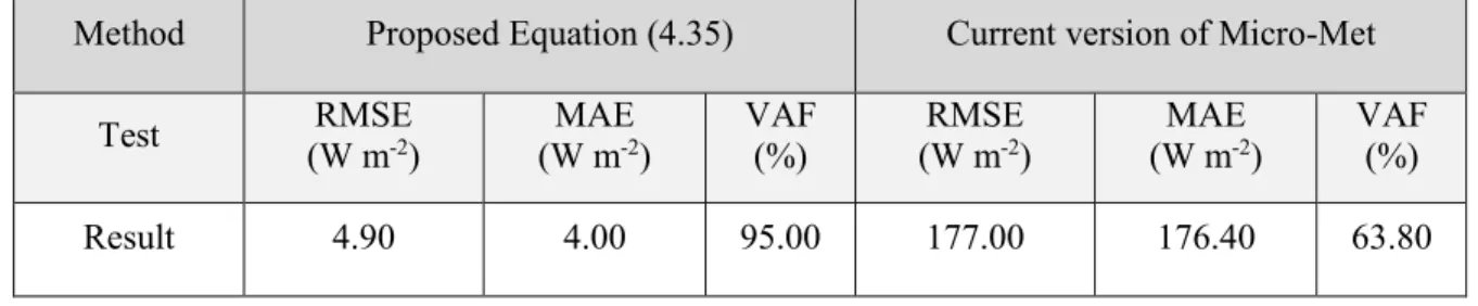
The second sub-model used observational data associated with synoptic conditions of radiation frost to present a locally adjusted downward longwave equation. The reported root means square error (RMSE) and mean absolute error (MAE) for the current version of Micro-Met were 176.95 (Wm-2) and 176.40 (Wm-2) respectively, while the results of the new equation led to an
RMSE and MAE of 4.90 (Wm-2) and 4.00 (Wm-2) respectively.
The third sub–model constituted three components: detected closed valley, estimated cold air drainage velocity, and integrated sensible heat loss and radiative cooling during the night on detected valleys. Comparison between the current Micro-Met simulation and the measured air temperature shows MAE of 1.11°C and RMSE of 1.66°C, while the comparison with the enhanced Micro-Met simulation indicated an improvement with MAE of 0.68 °C and RMSE of 1.08 °C. The fourth sub-model was based on experimental results of wind velocity produced in a laboratory with wind-tunnel models. Three separate equations were formulated for wind velocity estimation over the windward, through the shelterbelt, and leeward areas. The results indicated a coefficient of determination (R2) of 71% under the wind's velocity lower than 6ms-1.
The Enhanced Micro-Met version provided a new platform to power vegetation-atmosphere energy model to forecast minimum nocturnal temperature. The performance test for forecasting minimum air temperatures indicated agreement with in-situ measurements. Measurements were taken on five topographic sectors in order to assess the improved modeled prediction and led to error assessment
on closed valleys (RMSE=1.34, MAE = 1.03), different parts of slopes (RMAE = 0.93, MAE = 0.73), ridges (RMSE = 1.02, MAE = 0.88), flat areas (RMSE = 0.44, MAE = 0.40), and
areas close to the forest (RMSE = 0.58, MAE = 0.53).
In addition to previous specific objectives, this study proposed a new frost mitigation method based on the thermodynamics of water vapor transport from a moist source to dry sink. A vessel of warm water equipped with a Selective Inverted Sink (SIS) system was used to transport water vapor into the air, which ended up decreasing the air dryness and increasing moist entropy. This test was
III
carried out in an orchard. The most common mitigation method focuses on air temperature. Instead, the proposed method was based on the physical principles of moist entropy, which combined both air temperature and humidity and depicted heat content.
Overall, for this research project, a coupled model was designed to predict nocturnal minimum air temperature over hilly agricultural terrain. In particular, through improving prediction accuracy, we developed and added sub-models to estimate drops in temperature due to pooling and stagnation of cold air drainage and the effect of forest shelterbelt on wind velocity. To reduce frost effect, a new environmentally friendly active method was presented. This study served to help farmers reduce frost damages. Moreover, it can be useful for agricultural services in terms of decision-making, thereby, reducing economic damages.
Keywords: Radiation frost, Forecasting minimum air temperature, Spatial modeling, Cold air
drainage, Forest shelterbelt, Air temperature lapse rate, Net radiation, Frost mitigation, Moist enthropy.
IV
Resumè
Le gel radiatif est une des conditions météorologiques sévère affect la production agricole dans de nombreuses région du monde. Les objectives de cette étude inclut deux innovations scientifiques liées aux dégâts causés par le gel radiatif : (1) l'amélioration de la capacité de prédiction du gel local (température nocturne minimale à une résolution de 30 mètres) grâce à un modèle d’échange énergétique entre la végétation et l’atmosphère, et (2) une nouvelle méthode de diminution des risques et de protection des cultures agricoles pendant les périodes de gel.
La première innovation a été réalisée en suivant plusieurs objectifs spécifiques visant à améliorer les capacités d'un modèle de répartition spatiale météorologique (Micro-Met) via quatre sous-modèles : (i) estimation journalière du gradient thermique adiabatique de l'air, (ii) modification de l’équation de rayonnement des grandes longueurs d'onde en l’absence de nuage dans l’atmosphère, (iii) quantification des effets de l’écoulement de l’air froid sur la température de l’air, et (iv) quantifier l’effet de haies brise–vent sur la vitesse du vent. La deuxième innovation a été réalisée en mettant en œuvre et en testant une nouvelle méthode active basée sur le cycle thermodynamique. Le site d'étude se localise dans la région de Vallée de Coaticook de l’Estrie (Québec) subit les conséquences désastreuses du gel.
Le premier sous-modèle utilise une combinaison de profils de température provenant du satellite AIRS et de stations météorologiques afin d’estimer quotidiennement et régionalement le gradient thermique de l’air. L'utilisation de valeurs journalières, au lieu de valeurs fixes, permet d’estimer plus précisément les conditions atmosphériques. Les résultats ont démontré l’utilité de l’utilisation de la température de l'air obtenue par AIRS (850 hPa et 700 hPa) pour l’estimation du gradient thermique. Le second sous-modèle utilise les données associées aux conditions synoptiques du gel radiatif pour obtenir une équation du rayonnement descendant localement ajustée. Alors que l’erreur aux moindres carrés (RMSE) de Micro-Met était de 176.95 Wm-2 avec une erreur absolue
(MAE) moyenne de 176.40 Wm-2, la nouvelle équation génère une RMSE de 4.90 Wm-2 et une
MAE de 4.00 Wm-2. Le troisième sous-modèle contient trois parties :la détection des vallées
fermées, l’estimation de la rapidité de drainage de l’air, et l’intégration de la perte de chaleur sensible ainsi que le refroidissement radiatif en vallée durant la nuit. La comparaison entre les simulations Micro-Met et les mesures de la température de l’air montrent une MAE de 1.11 (°C) et une RMSE de 1.66 (°C). La comparaison avec le modèle amélioré indique un gain avec une MAE de 0.68 (°C) et une RMSE de 1.08 (°C). Le quatrième sous-modèle était construit sur des résultats expérimentaux de vitesse du vent générés en laboratoire par des simulations. Trois équations ont été proposées pour estimer la vitesse du vent. Les résultats indiquent un coefficient de corrélation (R2) de 71% pour une vitesse de vent en dessous de 6 ms-1.
La version améliorée de Micro-Net fournit une nouvelle plateforme pour des modèles d’énergie végétation-atmosphère et permet de prévoir la température minimale nocturne. Les résultats des tests de prédiction de cette température minimum concordent avec les mesures in-situ. Ces mesures ont été prises dans 5 secteurs topographiques différents afin d’améliorer les modèles de prédiction et engendrent des erreurs pour des vallées fermées (RMSE = 1.34, MAE = 1.03), pour différentes pentes (RMAE = 0.93, MAE = 0.73), crêtes (RMSE = 1.02, MAE = 0.88), plaines (RMSE = 0.44, MAE = 0.40), et aux orées des forêts (RMSE = 0.58, MAE = 0.53).
V
En plus des objectifs spécifiques précédents, cette étude a proposé une nouvelle méthode d'atténuation du gel basée sur la thermodynamique du transport de la vapeur d'eau d'une source humide à un puits sec. Nous avons ajouté au Selective Inverse System (SIS) déjà utilisé dans le milieu, un contenant d'eau chaude à sa base pour diffuser la vapeur d'eau dans l'air ambiant. Cette opération a augmenté l’humidité de l'air ambiant et augmenté l'entropie humide. Cet essai a été réalisé dans un verger. La méthode d'atténuation la plus courante se concentre sur la température de l'air. La méthode proposée repose plutôt sur les principes physiques de l'entropie humide, qui combinait à la fois la température et l'humidité de l'air et le contenu thermique représenté.
Dans l'ensemble, pour ce projet de recherche, un modèle couplé a été conçu pour prévision la température minimale nocturne de l'air dans des terrains agricoles vallonnés. En particulier, en améliorant la précision des prévisions, nous avons élaboré et ajouté des sous-modèles pour estimer les baisses de température dues à la stagnation du drainage de l'air froid et à l'effet des brise-vent forestiers sur la vitesse du vent. Pour réduire l'effet de gel, une nouvelle méthode de mitigation active respectueuse de l'environnement a été présentée. Cette étude a le potentiel d’aider les agriculteurs à réduire les dommages causés par le gel. De plus, elle peut être utile pour les services agricoles en termes de prise de décision, réduisant ainsi les dommages économiques.
VI
Acknowledgments:
I would like to present my sincere acknowledgement to Dr. Richard Fournier and Dr. Karem Chokmani for their support throughout my Ph.D. project. Without their contributions, my study would not have been possible. I would also express my appreciation to Caroline Turcotte from ministère de l'Agriculture, des Pêcheries et de l'Alimentation du Québec (MAPAQ). I would like to present my sincere acknowledgement to owners of Domaine Bergeville, Domaine Ives Hille, Verger Ferland, Bleuetière Mi-Vallon, Fromagerie La Station de Compton, and L'Abri Végétal. Their support was essential to establish a close connection between scientific research and practical agriculture and has been encouraging me during my research work.
VII
Content
1. General introduction ... 1
1.1 Theoretical background ... 3
1.1.1 Radiation and surface energy balance ... 3
1.1.2 Thermal inversion phenomena ... 5
1.2 Types of frost ... 5
1.3 Environmental variables linked to minimum air temperature and radiation frost ... 7
1.3.1 Meteorological variables ... 8
1.3.2 Effects of topographic variability, soil texture and forest ... 9
1.3.3 Plant characteristics ... 12
1.4 Frost protection methods ... 13
1.4.1 Passive methods for frost protection ... 13
1.4.2 Active methods for frost protection ... 14
1.5 Forecast of minimum temperature ... 15
2. Hypotheses, objectives and overview of the methodology ... 19
2.1 Hypotheses and objectives ... 21
2.2 Overview of the methodology ... 22
2.2.1 First component: providing meteorological data close to the sunset period ... 22
2.2.2 Second component: providing soil temperature close to the sunset period ... 23
2.2.3 Third component: vegetation-atmosphere model implementation ... 23
2.2.4 Fourth component: presenting a new frost mitigation method... 23
3. Experimental site ... 26
4.1 Introduction ... 29
4.2 Objective ... 34
4.3 Methodology ... 34
4.3.1 Modifying atmospheric emissivity equation under clear sky conditions ... 35
4.3.2 Estimation of the air temperature lapse rate ... 37
4.3.3 Quantifying the effects of cold air drainage on temperature ... 38
4.3.4 Quantifying the shelter effect on wind velocity ... 48
4.4 results ... 51
4.4.1 A modified downward longwave radiation equation during clear sky conditions ... 51
4.4.2 Estimation of air temperature lapse rate ... 53
4.4.3 Quantifying the effects of cold air drainage on air temperature... 54
VIII
4.4.5 Estimating temperature drops due to pooling of cold air ... 59
4.4.6 Quantification of the shelterbelt effect on wind velocity ... 63
4.5 Discussion and conclusion ... 67
5. Development of a method to predict soil temperature ... 74
5.1. Introduction ... 74
5.2. Study site and available data ... 76
5.3 Methodology ... 77
5.3.1 Spatial and temporal variability of the meteorological variables ... 77
5.3.2 Model input determination ... 78
5.3.3 Developing a short-term soil temperature predictive model ... 79
5.3.4 Model performance evaluation ... 79
5.4 results ... 80
5.4.1 Spatial and temporal variability of the meteorological variables ... 80
5.4.2 Data analyses and method input selection... 82
5.4.3 Soil temperature short-term estimation method ... 83
5.4.4 Assessing the performance of prediction methods ... 86
5.5 Discussion and conclusion ... 87
6. Modifications of the vegetation-atmosphere energy model to forecast nocturnal minimal air temperature ... 90
6.1 Description of the vegetation-atmosphere energy model ... 91
6.2 Methodology ... 93
6.2.1 Initialization ... 94
6.2.2 Processing functions ... 96
6.2.3 Model implementation and output ... 100
6.3 results ... 100
6.3.1 Estimation of the surface albedo ... 100
6.3.2 Estimation of the ground heat flux ... 101
6.3.3 Prediction of nocturnal minimum air temperatures ... 103
6.3.4 Performance of the model ... 106
6.4 Discussion and conclusion ... 107
7. Improvement of the method for the effectiveness of frost protection ... 110
7.1 Introduction ... 110
7.2 Methodology ... 112
7.2.1 Theoretical framework ... 114
7.2.2 Implementation process ... 116
IX
7.3.1 Observational evidence of the effects of the SIS system on air temperature ... 117
7.3.2 Results for the implementation of the new method... 121
7.4 Discussion and conclusion ... 121
8. Conclusion ... 125
8.1 Achievement of research objectives and innovative contributions ... 125
8.2 Summary of results ... 128
8.3 Research implications and future study... 129
9. References ... 131
Appendix A.1 Airs standard pressure levels (taken from GES DISC, 2016) ... 145
Appendix A.2 Wind speed variation as a function of distance from a windbreak and windbreak structure on the windward and leeward sides of a forest shelter (taken from Hanley and Kuhn (2003)) ... 146
Appendix A.3 Nomenclature of cold air drainage velocity equation ... 147
Appendix A.4 Estimation of cold air drainage velocity using proposed equation ... 148
Appendix A.5 Estimation temperature drop due to cold air drainage accumulation... 149
Appendix A.6 Extrapolated values for three areas : windward, over the forest and leeward areas based on distance and percentage of wind speed ... 154
Appendix B.1 Spectral range of a specific band of landsat ... 155
Appendix C. Specification of air and soil resistances ... 156
Appendix D. Model implementation when dew or rime deposit does not occur ... 157
Appendix E. Model implementation when dew or rime deposits occur ... 158
X
List of figures
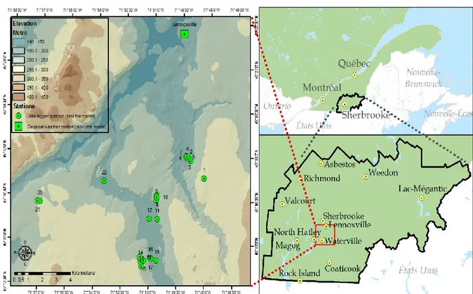
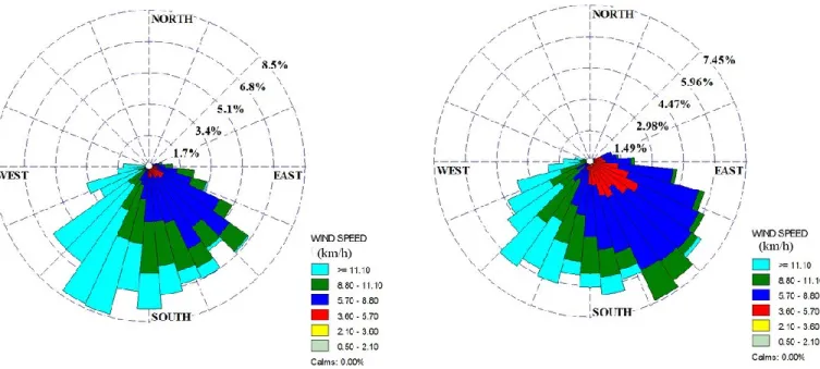
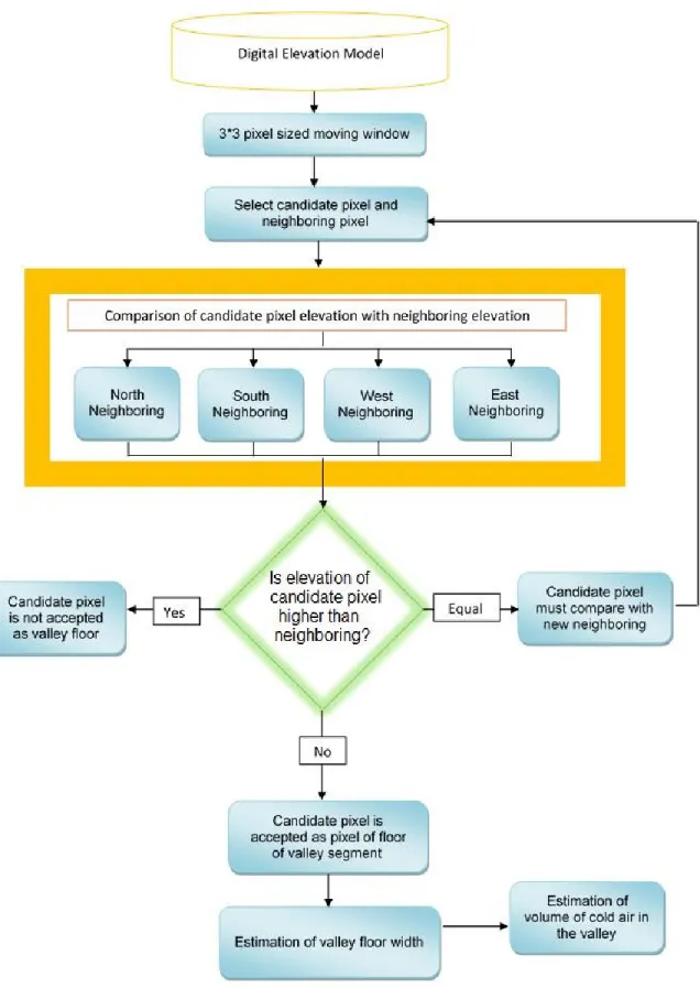
Figure 1.1 Percentage of damages due to climate-related disasters on between 2002 and 2007 (adapted from the world meteorological organization (WMO) report, 2010). ... 1 Figure 1.2 Schematics of the fluxes associated with the surface energy budget during a daytime when incoming solar radiation is present. The arrows indicate the direction of flux relative to the ground surface. Qs is incoming solar radiation. ... 4 Figure 1.3 Illustration of site topography effects on air temperatures during radiative cooling. The sinking cold air collects in low-lying areas and can create frost pockets, which are much more prone to spring and fall frost damages (taken from Snyder and Paulo Abreu, 2005). ... 14 Figure 1.4 Examples of different types of active methods against frost: (a) towerless wind machine also called selective inverted sink (SIS) system; (b) open-air heating; (c) helicopters; and (d) sprinkling irrigation. ... 15 Figure 1.5 Example of a frost alert issued by Environment and Climate change Canada for the eastern townships on a regional scale (Environment and Climate change Canada, 2017). ... 18 Figure 2.1 Diagram of the methodology procedure components: 1) enhanced micro-met, 2) soil temperature short –term estimation model, and 3) vegetation-atmosphere energy model to predict nocturnal minimum temperatures. ... 24 Figure 3.1 Location of the study site Coaticook river valley (Compton area). Position of weather station for the input data (square) and validation of the results (circles) are identified. ... 26 Figure 3.2 Land use map of the study site on a 225 km2 area. Land use classes in decreasing proportion are: Forest (53.63%), Agricultural (35.27%), Urban (7.41%), Other (3%) and Water (0.69%). ... 27 Figure 3.3 Heating degree-days (in yellow) and cooling degree-days (in blue) for the Lennoxville meteorological station based on 30 years data (Taken from Ministère de l'Agriculture, des Pêcheries et de l’Alimentation, 2017). ... 28 Figure 3.4 Wind rose for the study site. Left: May - june . Right: September - October . ... 28 Figure 4.1 Nasa illustration of scan geometry and coverage pattern for airs instruments on board the aqua satellite. Image courtesy of airs science team, NASA–California institute of technology (GES DISC, 2016). ... 38 Figure 4.2 Algorithm used to detect the area prone to accumulation of cold air drainage (depression areas) and their volumes. ... 40 Figure 4.3 An example of implementation of the algorithm to detect area prone to accumulation cold air drainage: red pixels correspond to the basin (width) of the valley floor, yellow to the flat pixels, and other colors to slopes. ... 41 Figure 4.4 A schematics of the forces that contribute to the cold air drainage flow over a simple slope during atmospheric stability conditions fg is gravitational force, fd is force exerted on the vegetation; fs is surface friction of the surface. The magnitude of fs is negligible compared with fd. ... 42 Figure 4.5 (a) An existing cold air layer with direction the white arrow is the direction of the cold air flow and shows, where the lake surface started. The cold-air flow came from the right-hand side of the picture and drained upon the lake; (b) an example of ultrasonic anemometers installation ... 43 Figure 4.6 Presentation of the study area (blackcurrant farm) and the slope where thermal imagery method presented, the red circle shows the experimental station and the yellow square, the thermal infrared camera location yellow lines show field of view. ... 44 Figure 4.7 Position of infrared camera on a blackcurrant farm and the slope. ... 44 Figure 4.8 Thermal photographs with color assigned temperature range allowing to visualize the fluctuation of cold air mass drainage on a slope at six different times (labelled on the upper left corner of each image). The red area shows isothermal temperatures bet ween -11.5 °c and -13 °c. ... 45
XI
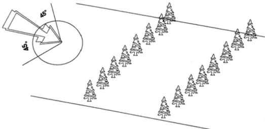
Figure 4.9 Shelter effect due to orientation of the rows of trees and the dominant wind direction (taken from Read et al., 1998). ... 49 Figure 4.10 Estimated wind velocity reduction on the windward (facing the direction from which the wind blowing, left side of treeline) and leeward (facing the direction toward which the wind is blowing) right hand side of the treeline. The distances from treeline are given in units for the treeline height (h) (taken from Van Eimern et al., 1964)... 50 Figure 4.11 Relative wind velocities in the vicinity of a large forest and the influence of shelterbelts on the
distribution of wind velocity expressed in percentages (taken from nageli, 1982). The red arrows (1 and 3) represent windward and leeward side respectively, while the blue arrow represents the portion through the forest. The black curve shows the wind velocity change (%) and the red curve shows shelterbelt of average penetrability. ... 51 Figure 4.12 Comparison of the air temperature retrieved by airs versus the radiosonde observation, (a) 925 hpa, (b) 850 hpa, and (c) 700 hpa. ... 54 Figure 4.13 a colour representation of the digital terrain model (DTM) of the study site with a spatial resolution of 10 m × 10 m. The low elevations are identified in blue and the high elevations in red or yellow. ... 55 Figure 4.14 Study area divided into two categories: (1) No valley including flat areas and open valleys (blue) and (2) Closed valleys (yellow shaded). ... 55 Figure 4.15 An example of applied equation 4.44 to derive field map of the cold air drainage velocity over closed valley; 18 october 2016, at 17:00. ... 57 Figure 4.16 Left figure shows two parallel lines over a 22-meter distance on a slope on a farm located on a sloped terrain in the study site on 5 november 2015; right figure shows temperature time series between lines R1 and R2. ... 58 Figure 4.17 A photo of the test area. The instrument used was decagon em50 (to measure surface temperature) and thermometer (to measure air temperature) at the bottom and top of the valley. ... 60 Figure 4.18 Hourly values of air temperature estimated with equation 4.32 (red) and measured (yellow) at the bottom of the valley on three night: 18-19 september (2016), 7-8 and 8-9 november (2017). Box plots indicate maximum/minimum values at the end of the wisker, the +/- 90% values with the end of the box and the average air temperature with the dot within the box. Air temperature values were estimated and measured one hour before sunset until ten hours after sunset. ... 60 Figure 4.19 An example of distribution of air temperatures simulated by current version of micro-met (a) and enhanced Micro-Met (b), at 17:00, 18 october 2016. ... 62 Figure 4.20 Comparison between measured and estimated (with the enhanced Micro-Met) air temperature values of a point in a low valley of the study site... 63 Figure 4.21 Curve fitting for the windward side. Horizontal distance from the shelterbelt expressed in tree height. ... 64 Figure 4.22 Curve fitting through the shelterbelt. Horizontal distance expressed in percentage of forest length. ... 64 Figure 4.23 Curve fitting for the leeward area. Horizontal distance from the shelterbelt expressed in tree height. ... 65 Figure 4.24 Comparison of the observed wind velocity versus those predicted using the enhanced
micro-met model. ... 66 Figure 4.25 Map showing the difference between the current version of met and the enhanced
micro-met which incorporated the shelterbelt sub model. The wind velocity recorded at the reference station (lennoxville) on 15 september 2016, at 19:00, was 7 kmh-1 s and 20 degree direction. ... 68 Figure 4.26 The identified areas prone to frost (in green), based on an upper limit threshold of 3.6 km/h applied to the enhanced micro-met system (left) and current version on micro-met (right). Yellow area
XII
experienced wind velocity more than 3.6 km h-1 and green area lower than 3.6 km h-1. Yellow area for Micro-Met was 154,622 m2 while the enhanced micro-met indicate 243,387 m2. ... 69 Figure 5.1 Location of the study site. The green circles show the position of the data loggers placed to measure soil and air temperatures, dew point, and wind speed. The green circles identify the location of the data loggers. ... 77 Figure 5.2 Air temperature, dew point, soil temperatures and soil humidity of the seven experimental stations during non-frost (oct. 6-7, 2012) and frost nights (oct. 8-9, 2012). Box plots indicate maximum/minimum values at the end of the wiskers, the +/- 90% values with the end of the box and the average air. ... 81 Figure 5.3 The observed and estimated soil temperature values (a) Stepwise (and Forward), (b) Backward (i), (c) Backward (ii), (d) Enter technics. ... 85 Figure 6.1 Schematic diagram and potential-resistance network for the one-dimension two-layer representation of energy transfers within and above the canopy (see nomenclature in Table.1 of Appendix E for definition of the symbols). ... 93 Figure 6.2 Flow diagram of the procedure of employed the vegetation-atmosphere energy model to predict nocturnal minimum temperatures. ... 95 Figure 6.3 Distribution map of the surface albedo at a 30-m spatial resolution over the study site, using the data from the landsat images and enhanced micro-met simulations (november 2016). ... 101 Figure 6.4 Fig. (a) shows distribution map of the net radiation flux at 17h00, 18 november 2016; and (b) ground heat flux, at 17:00, 18 november 2016 over the study site. ... 102 Figure 6.5 Time series of air temperatures recorded with an infrared camera on upper (l1) and bottom slope (l2) on 27-28 may 2016 (a) and 29-30 may 2016 (b). These figures show there were no periodic oscillations subsequent to minimum temperature point. ... 104 Figure 6.6 (a) Spatial distribution of the prediction of nocturnal minimum temperature (°c) over the study site (november 18-19, 2016). (b) spatial distribution over after appling cold air drainage model on prediction map. ... 105 Figure 7.1 Left: Selective inverse sink (SIS) system or upward-blowing wind machine. Right: parts of upward-blowing wind machine; 1.Fan chimney, 2.Fan kit, 3.Engine, 4.Construction 5.Protection cage (taken from Vardar and Taskin, 2014). ... 111 Figure 7.2 Left: Field measurement area of an orchard (cidrerie verger ferland). Right: observational network where black points represent the locations of the 53 data loggers to measure air temperature. ... 113 Figure 7.3 Left: Field measurement area of vineyard (le Domaine Bergeville) situated in study site. Right: observational network where circles represent the locations of the 30 data loggers to measure air temperature. ... 113 Figure 7.4 Schematic representation of forced convection provided by combined SIS system (worked at a 540-rpm speed). The red color show hot water reservoir. ... 114 Figure 7.5 Schematic representation of thermodynamic system. A given amount of water vapor transfer
from moist reservoir to steam cycle temperature at warm temperature tin .the cycle then carries this water vapor to a lower temperature tout where it is diffused into dry reservoir (from Pauluis
(2011)). ... 116 Figure 7.6 Selective inverted sink (SIS) system and water warm tank. ... 117 Figure 7.7 Air temperature patterns during the night of 29-30 september 2014 (Cidrerie Verger Ferland). The SIS system sign shows the location of the SIS system; strikethrough sign means “no SIS system operating” and normal sign means “SIS system operating”. ... 118
XIII
Figure 7.8 Air temperature pattern during SIS applying night of 28-29 october 2013 (le Domaine Bergeville). SIS sign show location of SIS; strikethrough sign means ‘no SIS operating’ and normal sign means ‘SIS operates. ... 119 Figure 7.9 Air temperature patterns during the night of 16-17 november 2013 (le Domaine Bergeville). The SIS system sign shows the location of the SIS system; strikethrough sign means "no SIS system operating" and normal sign means "SIS system operating". ... 120 Figure 7.10 Air temperature, specific humidity and moist entropy at 2m and 18m for two points: reference point and test point (14 may 2015) Cidrerie Verger Ferland. ... 122 Figure 7.11 Derivation of the airflow produced by the SIS system. The figure show that a minor part of the SIS system exhausted flux was from horizontal direction (small horizon sign) and major part of the flux was from the upper layer around the SIS system, which behaves like a funnel (ground sign). . 123
XIV
List of tables
Table 1.1 The flux density for each of the energy transfer terms for a citrus plant orchard. Under clear skies,
more heat is loss than gained (adapted data from bartholic et al., 1974, cited in mee, 1979). ... 7
Table 1.2 Examples of crops that may or may not resist to frost during different development stages. (taken from snyder and paulo de melo-abreu, 2005). ... 13
Table 2.1 Description of the data used in this study. ... 25
Table 4.1 air temperature lapse rate variations for each month of the year in the northern hemisphere (kunkel, 1989) used by the Micro-Met. ... 33
Table 4.2 Emissivity (Ε0) of clear-sky parameterizations suggested by different authors based on air temperature t (k), water vapor pressure ea (hpa), and precipitable water w (kgm-2). ... 36
Table 4.3 Coefficient values for the ten emissivity equations selected to fit the measured values under cloudless and low wind conditions at the sirene field station on 2014, 2015 and 2016 in sherbrooke (canada). We selected the days that reported 0-10% cloud cover. ... 52
Table 4.4 Statistics of downward longwave estimated using proposed equation versus results of current version of Micro-Met. ... 53
Table 4.5 Standard deviation, minimum and maximum values of measurement (meas) and estimated (estim) air temperature correspond to figure 5.19. Time presented by hour and started from one hour before sunset until ten hour after sunset. ... 61
Table 5.1 Geographical coordinates and topographical attributes for each of the experimental stations. .. 76
Table 5.2 Standard deviation of air, dew point, surface temperatures, and soil humidity for non- frost (oct.6-7, 2012) frost nights (oct.8, 9, 2012). ... 82
Table 5.3 Correlation coefficient between variable (air temperature, dew point temperature, soil moisture, wind speed, and absolute humidity) with soil temperature for experimental stations located on flat and depression areas. ... 83
Table 5.4 Comparison of linear and non-linear (quadratic and cubic). The Coefficient of determination (R2), and Standard Error of the Estimate (SEE) values do not show important difference amount the linear, quadratic and cubic. ... 84
Table 5.5 The selected methods and their mathematical functions in estimating soil temperatures at sunset time. For the nomenclature see Table 5.7. ... 86
Table 5.6 The nomenclature of different equations presented in Table 5.5. ... 86
Table 5.7 Statistical performance indices for different methods. ... 87
1
1. General introduction
The greatest agricultural risk in connection with low temperature is frost, which can cause severe damages to fruit, foliage, and plants. The danger of low temperatures in horticulture has been recognized since the beginning of farming. Thus, Romans considered the resistance to frost as an important factor when selecting species to cultivate in specific regions. They made efforts to protect crops from freezing injury nearly 2000 years ago during the first century AD (Columela, 1965). Frost is the occurrence of air temperature of 0°C or lower, measured at a height between 1.25 and 2 m above the ground within a weather shelter. Soil frost occurs when ice forms and soil may freeze. Soil frost and frozen depth can be variable and depends largly on early winter air temperature and the amount and timing of snowfall. Young vines, during establishment are particularly vulnerable to the soil frost (Snyder and Paulo de Melo-Abreu, 2005).
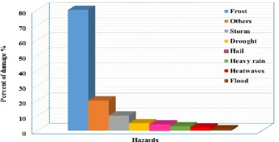
Based on the World Meteorological Organization (WMO), frost is one of the main disasters that limit agricultural production in many parts of the world. Damages caused by frost represent 80% of losses from climatic-related disasters (such as storm, hail, and flood) in agricultural sectors (Fig. 1.1). Consequently, frost can have serious impacts on our environment and society. In all parts of the terrestrial landmass, not including lowland tropics, frost is a cause for concern, because it affects the productivity of agricultural, horticultural and silviculture crops (Cohen, 1973; Bagdonas
et al., 1978).
Figure 1.1 Percentage of damages due to climate-related disasters on between 2002 and 2007 (Adapted from the World Meteorological Organization (WMO) report, 2010).
2
Forecasts for frost nights are usually limited to minimum air temperatures (Rodrigo, 2000; Richards and Baumgarten, 2003). Knowledge of the nocturnal minimum air
temperature constitutes one of the main variables during the agricultural period and can help farmers to mitigate its adverse effects on crop productivity through adequate measures. An effective implementation of any type of protection depends on a spatially accurate estimate of nocturnal minimum temperatures (Kalma et al., 1992).
The sensitivity of a crop to low temperatures depends on many factors including air temperature drop. Protecting plants from the effects of critical low temperatures is generally a matter of considerable importance in agricultural and especially horticultural production of high-value fruits and vegetables. Low temperatures and frost during the growing season cause stress, which may lead
to serious or irreversible damage of tissues or whole tree seedlings (Sakai and Larcher 1987; Blennow et al., 1998). This significant threat to farmers and gardeners has the potential to damage
plants, as well as the yield in some orchards (Gombos et al., 2011).
The early fall and late spring frosts usually cause damages to plants (Rosenberg et al., 1983; Geiger et al., 1995). In autumn, an earlier than normal frost can also destroy growing shoots or damage crops that are still in the field. However, the frost in the spring, more specifically at the end of the freezing period and at the beginning of the growing season, damages seedlings and young plants that are already at the flowering stage. Late frost in the spring can inflict a variety of damages,
depending on the development stage of the plant (Vestal, 1971; Rosenberg et al., 1983; Geiger et al., 1995). Frost can cause a rapid decline in net photosynthesis and stomatal conductance
rates. Young expanding leaves, reproductive organs, and other differentiating tree tissues are most sensitive to freezing temperatures (Taschler et al., 2004).
A wide range of active and passive method exist to avoiding or reducing frost damage. Passive method, such as plant selection, site selection, appropriate use of cultural and management practices; modification of microclimate of the crop are important to avert or minimize frost damage. However, under sever frost conditions, these methods are often inadequate to protect crops Active methods are implemented just before or during a frost night to prevent ice formation within sensitive plant tissue. Wind machines, sprinkling irrigation and open-air heating are the most common active protection methods (Snyder and de Melo- Abreu, 2005; Ribeiro et al., 2006).
The predicted trends in climate change, such as increasing temperature anomalies, may not altogether reduce the risk of frost. Most phenological models show that temperature rising in this
3
century can lead to earlier plant blossoming. In addition to the earlier start of the active vegetation period, the forecasted milder winters and early springs can multiply the risks of frost affecting buds, flowers, and fruit production (Eccel et al., 2008). By responding to warmer temperatures in early spring, plants face a risk of damaging fluctuations after bud break, which means that their vulnerability to low temperatures increases continuously.
1.1 Theoretical background
The earth’s surface is the main energy fluxes transfer area in the lower troposphere for many atmospheric, hydrological, and biological processes. Spatial variability in the surface fluxes is responsible for spatial patterns of meteorological variables and phenomena for a range of scales (Whiteman, 1990; Madelin, 2004). Following the laws of thermodynamics, energy can be transformed, transferred or stored, but not destroyed. Thus, the constant input of energy from the environment towards earth and object surfaces must be balanced with an equal output or be stored within interacting masses. The following section examines the forms of energy fluxes that occur to balance the net surplus or deficit resulting from the energy budget.
1.1.1 Radiation and surface energy balance
There are essentially four types of energy fluxes at the surface, namely (1) net radiation (Rn) to
or from the surface, (2) sensible heat fluxes (QH), (3) latent heat fluxes (QE) to or from the atmosphere,
and (4) ground heat flux (QG) into or out of land. Net radiation may be considered an external forcing,
while the sensible, latent, and ground heat fluxes constitute a response to this radiative forcing (Foken, 2008). In accordance with the principle of conservation of energy, for a unit horizontal area, the surface radiative surplus or deficit is balanced with a combination of convective exchanges to or from the atmosphere as sensible (QH) or latent (QE) heat, as well as through the conduction to or from
the underlying substrate such as the soil heat flux (QG). From this perspective, the complete energy
balance for a system corresponds to (Oke, 1987):
Rn= QH + QE + QG 1.1
Net radiation is usually positive during the day when the net shortwave (solar) input exceeds the net longwave (terrestrial radiative) loss; it is negative at night in the absence of solar radiation. Under clear skies at nighttime, more heat is radiated away from an orchard in the form of terrestrial radiation rather than receiving in the form of solar radiation, causing the soil temperature and consequently air temperature to drop (Snyder, 2000; Madelin, 2004). As the focus of this study is on the formation of
4
cold air at night, the mechanisms associated with heat loss are of primary interest. At night, the land surface loses energy through outgoing radiation, especially during clear skies. All the terms of the surface energy balance (Eq. 1.1) for land surfaces are usually negative during the evening and nighttime periods. As a result, the net radiation becomes negative in the equation for radiation balance, while the surface of the soil loses energy, due to the emission of thermal radiation. Several authors quantified these energy losses: the soil surface or that of a plant at 0°C emits radiation at about 300 Wm-2 or energy losses at approximately 2600000 kcal/hour. The net radiation term
typically is separated into parts representing the downward shortwave radiation from the sun, reflected shortwave radiation (upward), longwave downward radiation, and finally longwave upward radiation. These terms can be sketched on a surface energy budget diagram (Fig. 1.2) where the direction of the arrow designates the direction of energy transfer. The radiation budget for any point on the surface can be expressed as:
Rn = QS + QSR + QLu + QLd 1.2
where the net radiation (Rn) is calculated as the sum of the shortwave down welling radiation mainly
from the sun (QS), the longwave down-welling infrared radiation emitted by clouds, aerosols, and
gases (QLd), the shortwave up-welling reflected (solar) radiation (QSR), and the longwave up-welling
infrared (heat) radiation (QLu). The upward shortwave radiation is governed by the magnitude of
downward shortwave radiation and the proportion reflected as determined by the surface albedo (Liang et al., 2010). Upward longwave radiation made up of thermal radiation emitted from the surface and the portion of QLd are reflected as determined by surface emissivity. Shortwave radiation
can be divided into two types: diffuse radiation from the sky and direct solar radiation.
Figure 1.2 Schematics of the fluxes associated with the surface energy budget during a daytime when incoming solar radiation is present. The arrows indicate the direction of flux relative to the ground surface. QS is incoming solar radiation.
5
The loss of energy from the ground can be limited by atmospheric radiation to the earth. This limitation is of greater importance when the atmosphere has higher relative humidity. Water vapor absorbs the terrestrial radiation and reduces its escape to the space. Low-altitude cloud formations always indicate a high level of humidity in the lower levels of the atmosphere. Therefore, during cloudiness condition, a significant fraction of the radiation emitted from the ground is absorbed in the clouds and reradiated back into the ground. Thus, clouds reduce the radiation imbalance between the upward flux from the ground and downward flux from the atmosphere. Conversely, when the atmosphere is dry and clear, the downward atmospheric radiation is less than that emitted by the earth and the energy balance is negative. The radiative and energy balances are then close to zero and the air-cooling is minimal. For example, consider the energy balance of a vegetated surface with a zero temperature for two different conditions: clear sky and cloudiness. For the clear sky, atmospheric radiation is no more than 200 Wm-2. However, the terrestrial radiation (infrared radiation) is 300 Wm -2. The radiative surface energy balance is -100 Wm-2. Under a clear sky, more heat is lost than gained
in this process. Dry air is transparent to infrared radiation, allowing energy to escape from the surface. 1.1.2 Thermal inversion phenomena
The troposphere is the atmospheric layer where on average, the air temperature decreases with increasing altitude. The change of air temperature with altitude is referred to as the air temperature lapse rate and, which will vary on any given day. During the nighttime hours, there is a net loss of longwave radiation from the surface to the sky. Sensible heat content of the soil decreases as energy is radiated away, causing the air temperature near the surface to drop. Because there is a deficit of sensible heat near the surface, there is sensible heat transfer by conduction from the air above to partially replace the surface heat loss. Therefore, the radiative cooling due to longwave radiation leads to the progressive thickening of the surface inversion layer and leading to temperature increase with altitude and the value of the lapse rate to be negative (Goplakrishnan and Shran, 1998). This phenomenon, which occurs under negative net radiation and low winds, is called a thermal inversion (Snyder and Paulo de Melo-Abreu, 2005). An inversion acts as a ceiling, preventing further upward convection, which is generally the limit for cloud development (Madelin, 2004).
1.2 Types of frost
Frost is formed through two types of physical processes: radiative or advective cooling which lead to two dominant types of frost situations, advection and radiation frosts (Tait and Zheng, 2003).
6
Each type is associated with different frost management strategies. Regardless, understanding the physics these two processes is critical to develop efficient frost management strategies.
Radiation frost is characterized by clear sky, no wind, and low dew point temperature.
Radiation frosts occur at night and result from intense, longwave radiation cooling under calm, clear and dry atmospheric conditions. Strong surface inversions develop in the stable atmosphere associated with radiation frosts. It occurs because of heat losses in the form of radiant energy. Under a clear nighttime sky, more heat is radiated away from an orchard than it is radiated into the orchard. Consequently, the temperature drops faster near the radiating surface, causing a temperature inversion during radiation frost conditions. Energy is lost through radiation upward from the surface. It is channeled through downward radiation from the sky, conduction of heat upward through the soil, and convection of warmer air to the colder plants. Table 1.1 shows a typical nighttime energy balance for a citrus plant orchard. The values are comparable to other crops. Under a clear sky, more heat is lost than gained in this process.
Advection frost is characterized by moderate or strong cold wind (at least 2 ms-1 or more),
below critical temperatures, which are part of large regional cold air masses. Destructive cold temperature events under advective (windy) conditions are often called freezes rather than frosts. These large-scale winds have a tendency to persist throughout the night and sometimes during the day. They may occur under cloudy or clear sky. Windy conditions do not permit thermal inversions to form although radiation losses are present. The rapid cold air movement that advects or “steals away” the heat from the plant causes damages. Advective frosts are characterized by cloudy skies, moderate to strong winds, no temperature inversion, and low humidity.
Very little can be done to protect plants against advective-type frost. Placing trees under water sprinklers is suggested as one of the few alternatives to avoid the effects of advection frost. Water
transition from its liquid phase into ice lead to release the latent energy into sensible energy (334 kJ kg-1). By this way, we use the energy produced by transition of water, when the air
temperature is below freezing points (0°C). There are two differences between radiation and advection frosts: (i) Under radiation frost conditions, winds are normally light and temperature inversions develop as the air in contact with the cold radiating surfaces becomes chilled and heavy. However, Advection frosts often occur with strong winds. (ii) Since advection frost is caused by the passage of a cold front, it generally occurs at a regional or synoptic scale. However, radiation frost is a local phenomenon. This is why the use of spatially explicit models can help to identify the risk areas
7
(Ahrens, 2000). Even though both types of processes are usually present in most frost events, radiation frost is the dominant type of frost during the growing period (Snyder and Paulo de Melo-Abreu, 2005).
Table 1.1 The flux density for each of the energy transfer terms for a citrus plant orchard. Under clear skies, more heat is loss than gained (Adapted data from Bartholic et al., 1974, cited in Mee, 1979).
Energy Transfer Flux Density (Wm-2)
Conduction (from the soil) +28 Convection (from the air) +39 Downward Radiation (from the sky) +230 Upward Radiation (from the orchard) -315 Net Energy Loss from the crop -18
1.3 Environmental variables linked to minimum air temperature and radiation frost
There are many factors that can affect near-surface air temperatures across regions in complex terrains. The orography, the soil and vegetation characteristics, as well as local variations in net radiation, may all play a part in determining the temperature distribution. Their relative importance will vary according to large-scale climate conditions. Many studies have reported the role of environmental variables related to frost, more specifically regarding meteorological and geographical variables. For example, Bootsma (1976) studied the minimum temperatures and risks of frost in the mountainous lands of Canada. The results indicated that the average estimated frost date occurring in valley bottoms was 34 days later in the spring and 39 days earlier in the fall compared to higher elevations. Avissar and Mahrer (1988) developed a three-dimensional model to simulate the local scale microclimate zones near ground level during radiative frost nights in non-uniform lands. Effective variables of this model included topography, vegetation, soil humidity, wind velocity and direction, and air humidity.
Field research over open areas shows that minimum temperature changes with elevation, wind velocity, and total net radiation at night (Kajfez, 1987). Nocturnal temperature varies at fine spatial scales in complex terrain, reflecting interactions of synoptic atmospheric conditions with terrain, vegetation and spatial location (Gombos et al., 2011). Three types of variables can influence frost damage risk and its severity: (1) meteorological variables (2) topographical variability, and (3) plant characteristics.
8
1.3.1 Meteorological variables
Important meteorological variables such as air humidity, cloud cover effect, wind velocity, must be considered to understand how they are connected to air temperature and frost.
Air humidity: Air humidity represents the amount of water vapor in the atmosphere and
influences the surface radiation budget, consequently air temperature. Atmospheric humidity is expressed in a variety of ways, many of which have emerged from the meteorological research community. Some of the most common variables to express atmospheric humidity include dew point, specific humidity, and relative humidity. The humidity contained in the air absorbs part of the terrestrial radiation, which is then partly reemitted towards the ground. Therefore, the air humidity could then reduce the radiative deficit through an increase of atmospheric radiation during the night. In addition, the water vapor effect on the dew point temperature combined with condensation consequently releases latent heat energy. The presence of humidity limits radiative cooling, whereas dry air can enhance cooling by facilitating evaporation on soil and plant surfaces.
Cloud cover: Cloudiness is regarded as a key variable affecting the Earth's radiation balance
and therefore, the difference in nocturnal cooling rates (Kidder and Essenwanger, 1995; Gustavsson, 1990). Clouds dense enough to cast a shadow on the ground emit longwave radiation like full radiators at the cloud base temperature of the water droplets or ice crystals from which they are formed. The presence of clouds increases the flux of atmospheric radiation received at the surface, because the radiation from water vapor and carbon dioxide in the lower atmosphere is supplemented by the emission from clouds in the wave band, particularly between 8 and 13 µm. For clear skies, the heat loss at the ground level is greater than during nights when the sky is partly covered. In summary, solar and terrestrial radiation depend on the amount and types of clouds.
Wind velocity: Wind velocity corresponds to another climatic variable in connection with
nocturnal cooling. Wind direction determines the characteristics of air mass (temperature, humidity) on the synoptic scale. Vazart (1988) demonstrated an increased risk of frost through the advection of
cold and dry air after a rainfall or snowfall (advection frost). The low speed of the wind (less than 2 ms-1) is not able to enhance the mixing of the atmospheric layers and in particular, the low
layers where the phenomenon of thermal inversion occurs. In the case of light winds and clear skies,
the amount of turbulent heat transported downward is less than higher wind speed condition (Van de Wiel et al., 2012). Hence, wind speed exercises influence on air temperature differences.
9
but light winds can disturb cold air stagnation. During windy nights, the minimum temperature is therefore higher than during nights with light winds.
1.3.2 Effects of topographic variability, soil texture and forest
Topographic variation has a significant effect on climate on a scale of tens to hundreds of meters (Tran, 2017). The nocturnal temperature and severity of frost varies considerably with general atmospheric conditions, as well as with local differences in topography and vegetation (Richards and Baumgartner, 2003). Topography has two major effects on frost and ground-level temperature distribution: the first is tied to hill slope angle and aspect, while the second is related to local relief creating wind patterns and generation of air flow. Zinoni et al. (2002) conducted a climatological and orographic study to identify areas prone to frost and determine the characteristics of frost events between April 1987 and March 2000 for 161 weather stations in the Emilia-Romagna region in Italy. They determined correlations among climatic and orographic variables and defined a significant correlation between the mean minimum air temperature during the frost and the relative height from valley bottom. Moreover, a minimum temperature map was derived over New Zealand using GIS modeling and relied on factors such as ground cover, slope, elevation, latitude, and distance from the sea (Richards and Baumgarten, 2003). Their results highlighted that spatial distribution of radiation frost is closely associated with topographic patterns.
Focusing on late frost spatial modeling, the air temperature was measured using thermal infrared images during a strong thermal inversion episode in a fruit-growing area (Eccel et al., 2008). Their results indicate the existence of a clear geographic pattern in the distribution of minimum air temperature. With regard to the above mentioned, several other studies have documented the importance of local topography in causing large temperature variations, assessing severity and spatial distribution of radiation frost (Tabony, 1985; Bogren and Gustavsson, 1989; Toritani, 1990; Whiteman et al., 2007; Barry, 2008). All of these studies bring attention to the role of microclimate and geographical parameters related to frost risk.
As a conclusion, the severity of radiation frost varies with general atmospheric conditions, as well as local differences in topography. Primary topographic effects result from differences in hill slope angle and aspect, while secondary effects can result from the influence of terrain on mountain winds and generation of air flow effects such as cold air-drainage (Barry, 2010). Along with the changes in the topographic amplification in the valley, several factors need to be considered to determine whether or not the cold air in the valley is likely to drain.
10
Drainage flows are caused by the rapid cooling of the air after sunset in contact of air flow from surrounding terrain slopes. This air is negatively buoyant and pushed down the slopes towards the bottom of the valleys, following gravity. Cooling during the night caused by radiation is why cold air from mountains and slopes descends under gravity into valleys (Fohn, 2006).
The resulting horizontal buoyancy gradient drives a flow in a downslope direction, transporting air toward the valley bottom. The down-slope movement of air is referred to as katabatic wind. Local down-slope gravity flows are known by several names, particularly cold air drainage, cold air run-off, cold air stream, and cold air current (Geiger, 1965). Cold air flow, as well as in situ cooling, contributes to nocturnal cooling in a valley. Cold air tends to sink in the valleys; moreover, there are much lower temperatures than the corresponding free air. This phenomenon is called a “cold-air pool.” The significant temperature anomalies experienced in such zones can have strong impacts on
local native plant distributions, as well as horticulture and agriculture (Chung et al., 2006; Hubbartet et al., 2007; Bigg et al., 2014).
A number of studies have contributed important knowledge about the physical processes controlling nocturnal cold air drainage. External meteorological factors that influence the magnitude of cold air drainage and nocturnal winds were identified by Barr and Orgill (1989). Physical mechanisms of heating and cooling related to cold air drainage in a single basin described (Kondo et al., 1989; Konno et al., 2013). Chung et al. (2006) presented a statistical approach to estimate the effect of cold air accumulation on local temperature variations for a small basin. The results indicate that eliminating cold air drainage in spatial estimation of nocturnal air temperature was a source of uncertainty and error. These studies and others (Dobrowski et al., 2009; Lundquist and Cayan, 2007) demonstrate that cold air drainage and cold-air pool are physically interpretable processes that occur across diverse topographic areas.
Most theoretical analyses on cold air drainage flow are reduced to bare slope conditions. Cold air drainage flow also depends on the vegetation cover. For this reason, a complete model remains to be developed for cold air drainage flow by taking all the significant aspects of relief and land cover into account (Gaulden et al., 2007). However, direct objective measurement and modeling of cold air pooling requires micrometeorological observations and modeling techniques that were unavailable (Lundquist et al., 2008). Despite the growing awareness of influence of cold air drainage on nocturnal temperature, this phenomenon is not considered on currently interpolation methods.
11
In addition to local topography, soil texture plays a role in the net radiation balance and air temperature variations, because each type of soil comprises unique textural characteristics. Sandy soils warm up more rapidly in the spring than clay soils. This is due to lower heat capacity, lower thermal conductivity, and less evaporative chilling. Soil texture is defined by the relative volume of sand, silt, and clay particles. Longwave radiation emission by the surface is lower when the soil is wet and has vegetation cover. Coarse texture has poor heat capacity and therefore emits more longwave radiation than fine texture. The thermal regime of the soil can be modified by regulating
incoming and outgoing radiation, as well as by changing the thermal properties of the soil (Baver et al., 1972).
Mass density, specific heat, heat capacity, thermal conductivity, and thermal diffusivity are the thermal properties relevant to heat transfer through soil. These properties affect on average soil temperature or distribution of temperature in the soil. Thermal conductivity is affected by soil moisture and texture. Wet soils have higher conductivity than dry ones. Moreover, soil texture determines how quickly the soil will heat or cool. Therefore, the energy flux transmission within the soil depends on the physical properties of soil particles, their degree of compaction, and soil moisture content.
Understanding modifications to the microclimate due to wind shelters has been an active area of research for several decades (Hipsey et al., 2004). The influence of the forest shelterbelt on nocturnal temperatures can help formalizing to predict local frost. The primary effect of shelterbelts is the reduction in wind speed, which causes reduced air turbulence or mixing (during day and night). However, when the surface cools at night, reduced mixing causes lower minimum temperatures, compared with open areas. The sheltered zone has a modified microclimate and generally greater crop yields. The wind velocity reduction tends to decrease air and surface temperatures, partly by preventing the breakup of the atmospheric inversion (Monson, 2014).
The sheltering mechanism relies on the reduction of turbulent mixing of the cold near-surface air with warmer air aloft. Under clear conditions, this leads to a higher rate of cooling of the air in contact with the radiative cooling surface (Gustavsson et al., 1998; Monson, 2014). The magnitude of temperature change in a sheltered zone may reach up to 2°C. The reduction of wind velocity in the protected areas behind a shelterbelt takes place because the shelterbelt exerts a drag force on the wind field, leading to a loss of momentum of the airflow (Plate, 1971). This results in altered microclimates in protected areas. Shelterbelts and windbreaks remain an important area of research
12
in field, wind tunnel and numerical studies (Rajewski, 2007). Experimental studies of wind speed and turbulence were done in laboratories with wind-tunnel models and in the field with full-scale models. Van Eimern et al. (1964), McNaughton (1988), and Heisler and Dewalle (1988) provided interpretations of experimental data. The effect of forest shelter on wind velocity reduction and turbulence intensity, depends on its structure such as width, length, shape (Vigiak et al., 2003; Lee, 2010), and porosity (Santiago et al., 2007; Lampartova et al., 2015). Most shelterbelt studies reported in the literature are experimentally driven, emphasizing wind-speed reduction produced by shelterbelts. Therefore, effects of the forest wind shelter are divided into two functions: directly related to the effect on wind velocity and indirectly related to air temperature due to the effect of wind velocity.
The prediction methods must add some spatial algorithms in order to account for local terrain effects. Local topography effects can result from the influence of terrain relief on wind and generation of airflow such as cold air drainage. An understanding of terrains related process such as sheltering and cold air drainage is required to improve nocturnal short-term weather predictions.
1.3.3 Plant characteristics
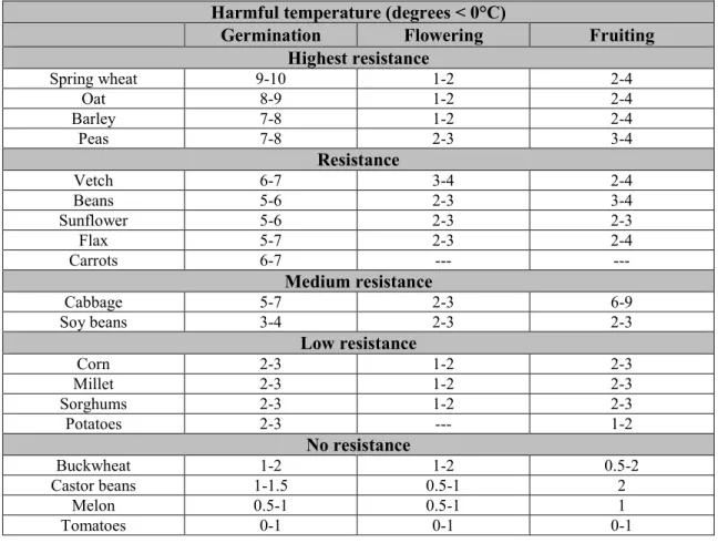
Plant characteristics such as the type, variety, and stage of development show that plant species differ greatly in their susceptibility to cold injury (Table 1.2). Crops are particularly prone to damage due to low temperatures during certain stages, especially flowering and early reproductive developments. During these periods, temperatures below the freezing level may damage the plants, while temperatures just above the freezing level might slow down plant growth. Frost damage occurs as water within plant cells freezes.
The air temperature at which this happens varies depending on the plant part and biochemical characteristics that change during the development of the plant. The level of tolerance to frost of a plant or the minimum air temperature at which a plant can withstand serious injury is referred to as the critical temperature (Snyder and Paulo de Melo-Abreu, 2006; Olszewski et al., 2017). Protecting plants from the effects of destructive low air temperature is generally a matter of considerable importance in agriculture, especially in terms of horticultural protection of high-value fruits and vegetables.
13
Table 1.2 Examples of crops that may or may not resist to frost during different development stages (taken from Snyder and Paulo de Melo-Abreu, 2005).
Harmful temperature (degrees < 0°C)
Germination Flowering Fruiting
Highest resistance Spring wheat 9-10 1-2 2-4 Oat 8-9 1-2 2-4 Barley 7-8 1-2 2-4 Peas 7-8 2-3 3-4 Resistance Vetch 6-7 3-4 2-4 Beans 5-6 2-3 3-4 Sunflower 5-6 2-3 2-3 Flax 5-7 2-3 2-4 Carrots 6-7 --- --- Medium resistance Cabbage 5-7 2-3 6-9 Soy beans 3-4 2-3 2-3 Low resistance Corn 2-3 1-2 2-3 Millet 2-3 1-2 2-3 Sorghums 2-3 1-2 2-3 Potatoes 2-3 --- 1-2 No resistance Buckwheat 1-2 1-2 0.5-2 Castor beans 1-1.5 0.5-1 2 Melon 0.5-1 0.5-1 1 Tomatoes 0-1 0-1 0-1
1.4 Frost protection methods
If economic conditions prevail, crops can sometimes be protected against frost. A wide range of passive (indirect) and active (direct) methods exist to avoid or reduce frost damage (Kalma et al., 1992; Snyder and Paulo Abreu, 2005). Most of these frost protection methods are practical and effective only against radiation frost.
1.4.1 Passive methods for frost protection
Passive protection includes methods that are implemented before occurrence of radiation frost to help avoid the need for active protection. This method used well in advance before the actual freeze danger is probably the most economical and effective. The most widely employed forms of these methods include site selection, managing cold air drainage, plant selection, plant nutritional management, and bacteria control (Snyder and Paulo Abreu, 2005). The main passive method is site selection. A given farm may have one or more natural microclimates where minimum temperatures
14
during frost events are much warmer or colder than those in the surrounding areas. For example, under radiative cooling conditions, the earth loses heat to space and cools the adjacent layer of air. If the vineyard is on a slope, the cold, relatively dense air moves downhill (Fig. 1.3). The sinking cold air collects in low-lying areas and can create frost pockets. The vineyards in low-lying frost pockets are much more prone to frost damage, than the ones at higher elevations one. Therefore, agricultural producers should use passive protection methods such as sites selection before planting is established. In fact, good cold air drainage management and planning is an important part of freeze protection programs from the beginning.
Figure 1.3 Illustration of site topography effects on air temperatures during radiative cooling. The sinking cold air collects in low-lying areas and can create frost pockets, which are much more prone to spring and fall frost damages (taken from Snyder and Paulo Abreu, 2005).
1.4.2 Active methods for frost protection
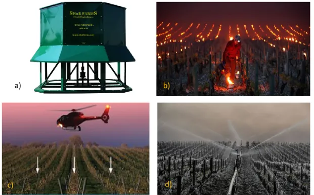
Active protection takes place just before and during a frost event, specifically after a frost warning has been issued in the weather forecast. The use of wind machines Selective inverted sink (SIS) system, open-air heating, sprinkling irrigation, and helicopters are the most common active protection methods (Fig. 1.4). The tower-less wind machine, also known as SIS system, was designed to drain cold air to prevent it from accumulating. In spite of the various methods adopted to prevent frost, the damage to plants continues to pose a problem and exert a major economic impact. Implementing frost protection at the wrong time or under the wrong conditions may sometimes be more damaging than doing nothing at all. Consequently, an efficient implementation of any type of protection depends on a spatially accurate estimate of frost. Reliable knowledge of the minimum air temperature can help farmers to mitigate its adverse effects on crop productivity by taking adequate
15
measures. There are methods available to protect against and to prevent frost, but they need to be implemented before the frost actually occur.
Farmer should know the nocturnal temperature variation as they occur over their land which fields are most prone to forest, so that action can be taken in these fields.
Figure 1.4 Examples of different types of active methods against frost: (a) towerless wind machine also called selective inverted sink (SIS) system; (b) open-air heating; (c) helicopters; and (d) sprinkling irrigation (taken from Snyder and Paulo de Melo-Abreu, 2005).
1.5 Forecast of minimum temperature
For efficient implementation of frost protection strategy, high resolution and accurate forecasts of minimum air temperatures are required, (Kalma et al., 1992; Blennow and Persson, 1998; Prabha and Hoogenboom, 2006). Reliable forecasts are of considerable importance in the agricultural field to identify frost conditions and facilitate the implementation of protective measures (Rodrigo, 2000; Lhomme and Guilioni, 2004). Knowledge of the nocturnal minimum air temperature constitutes one of the main variables during the agricultural period and can help farmers to mitigate its adverse effects on crop productivity through adequate measures. Predictions of nocturnal minimum temperatures and warnings enable horticulturists to make good decisions in terms of frost protection (Taboni, 1985).
a) b)
16
Forecasting the high-spatial resolution of air temperature in complex terrains represents an important scientific challenge. Current frost forecasting models only offer low spatial resolution. Studies using low-resolution climate models could not capture high-resolution interactions such as topography, vegetation cover, and cold air drainage, which are key factors of frost occurrence (Fleagle, 1950; Kalma et al., 1992).
Various authors have produced a vast number of empirical formulae to predict minimum air temperature. Early methods of prediction were mainly based on statistical relations between nocturnal temperature decreases and meteorological variables (Young, 1920; Ellison, 1928). Relevant meteorological variables generally included some expression of air humidity and possibly cloud coverage. These empirical methods have only local predictive potential, but they have not really been applied to other locations (Cellier, 1993). Following Brunt’s approach (1941), many simplified formulae were published based on the analytical solution of the heat conduction equation in bare soil (Jacob, 1940). However, they were developed for open areas or plains. This means that for the
topographic regions with, these methods did not produce reliable predictions (Ghieliand and Eccel, 2006). Another approach adopted refers to the artificial neural network, which is
empirically based and does not take into account the physical and dynamic aspects of land-atmosphere interactions or their temporal evolutions (Prabha and Hoogenboom, 2008). Other approaches based on the vegation-atmosphere energy balance designed by Shuttleworth and Wallace (1985), and upgraded by Shuttleworth and Gurney (1990), were used to predict the minimum air temperature from observations made during the sunset transition period (Lhomme and Guilin, 2004). Yet these modeling approaches do not consider the local circulations due to topography such as cold air drainage (Whiteman et al., 2010).
Forecasting frost with a weather prediction model at the mesoscale reduced prediction errors when compared with earlier models. Nevertheless, numerical weather prediction (NWP) models are mostly generalized, thus the NWP data is not useful for rural areas where farming is dominant (Huth, 2004). Furthermore, Environment and climate change Canada has the responsibility to call all meteorological alerts. Frost warnings issued by Environment and climate change Canada on a regional scale (~15 km) are not presented in a format suitable to interpretation for a specific site or farm. Instead, the alerts are issued at a regional scale, for example the Coaticook area or Brome-Missisquoi area (Fig. 1.5). Conversely, the assessment of the agricultural production loss at a farm or on a local scale requires access to compatible frost information.