Les Cahiers de la Chaire Economie du Climat
Fostering Renewables and Recycling a Carbon Tax: Joint
Aggregate and Intergenerational Redistributive Effects
Frédéric Gonand
1A rising share of renewables in the energy mix pushes up the average price of energy - and so does a carbon tax. However the former bolsters the accumulation of capital whereas the latter, if fully recycled, does not. Thus, in general equilibrium, the effects on growth and intertemporal welfare of these two environmental policies differ. The present article assesses and compares these effects. It relies on a computable general equilibrium model with overlapping generations, an energy module and a public finance module. The main result is that an increasing share of renewables in the energy mix and a fully recycled carbon tax have opposite (though limited) impacts on activity and individuals’ intertemporal welfare in the long run. The recycling of a carbon tax fosters consumption and labour supply, and thus growth and welfare, whereas an increasing share of renewables does not. Results also suggest that a higher share of renewables and a recycled carbon tax trigger intergenerational redistributive effects, with the former being relatively detrimental for young generations and the latter being pro-youth. The policy implication is that a social planner seeking to modify the structure of the energy mix while achieving some neutrality as concerns the GDP and triggering some proyouth intergenerational equity, could usefully contemplate the joint implementation of higher quantitative targets for the future development of renewables and a carbon tax fully recycled through lower proportional taxes.
JEL classification: D58, D63, E62, L7, Q28, Q43
Keywords : Energy transition, intergenerational redistribution, overlapping generations, carbon tax, general equilibrium.
n° 2014-08
Working Paper Series
1. University of Paris-Dauphine (LEDa-CGEMP) and Climate Economics Chair
I am indebted to Pierre-André Jouvet, Patrice Geoffron, Alain Ayong Le Kama, Jean-Marie-Chevalier, the participants of the FLM meeting of the Climate Economic Chair, Boris Cournède, Peter Hoeller, Dave Rae, David de la Croix, Jørgen Elmeskov for useful comments and discussions on earlier drafts. All remaining errors are mine.
Fostering Renewables and Recycling a Carbon Tax: Joint
Aggregate and Intergenerational Redistributive Effects
Frédéric Gonand
∗April 25, 2014
Abstract
A rising share of renewables in the energy mix pushes up the average price of energy -and so does a carbon tax. However the former bolsters the accumulation of capital whereas the latter, if fully recycled, does not. Thus, in general equilibrium, the effects on growth and intertemporal welfare of these two environmental policies differ. The present article assesses and compares these effects. It relies on a computable general equilibrium model with over-lapping generations, an energy module and a public finance module. The main result is that an increasing share of renewables in the energy mix and a fully recycled carbon tax have op-posite (though limited) impacts on activity and individuals’ intertemporal welfare in the long run. The recycling of a carbon tax fosters consumption and labour supply, and thus growth and welfare, whereas an increasing share of renewables does not. Results also suggest that a higher share of renewables and a recycled carbon tax trigger intergenerational redistributive effects, with the former being relatively detrimental for young generations and the latter being pro-youth. The policy implication is that a social planner seeking to modify the structure of the energy mix while achieving some neutrality as concerns the GDP and triggering some pro-youth intergenerational equity, could usefully contemplate the joint implementation of higher quantitative targets for the future development of renewables and a carbon tax fully recycled through lower proportional taxes.
JEL classification: D58 - D63 - E62 - L7 - Q28 - Q43.
Key words: Energy transition intergenerational redistribution overlapping generations -carbon tax - general equilibrium.
E-mail : [email protected] Phone: (00)+33(0)682450952. I am indebted to Pierre-André Jouvet, Patrice Geoffron, Alain Ayong Le Kama, Jean-Marie-Chevalier, the par-ticipants of the FLM meeting of the Climate Economic Chair, Boris Cournède, Peter Hoeller, Dave Rae, David de la Croix, Jørgen Elmeskov for useful comments and discussions on earlier drafts. All remaining errors are mine.
1
Introduction
A rising share of renewables in the energy mix pushes up the average price of energy - so does a carbon tax. However the former fosters the accumulation of capital while the latter, if fully recycled, does not. Thus the effects of these two environmental policies on growth and on intertemporal welfare for different cohorts policies differ. The present article assesses them.
General equilibrium (GE) analysis applied to energy issues has been developing since the 1970’s. Sato (1967) and Solow (1978) popularized GE frameworks with CES production functions including energy as a third input. Energy-related computable GE models have been commonly used (e.g., Per-roni and Rutherford (1995), Böhringer and Rutherford (1997), Grepperud and Rasmussen (2004), Wissema and Dellink (2007)). Knopf et al. (2010) present different CGE models encapsulating an energy sector with a rising share of renewables in the energy mix, in order to assess empirically the long-run costs of meeting the 450ppm environmental objective. However, these models are not specifically designed to address issues such as the dynamics of the year-to-year effects on growth of environmental tax reforms and their implied intergenerational effects.
Some litterature focuses on the dynamics of environmental taxation in a general equilibrium setting and their intergenerational redistributive effects. It takes account of its impact on the in-tertemporal consumption/saving arbitrage and the capital intensity of the economy. To this end, John et al. (1995) rely on an overlapping generations (OLG) framework. OLG settings allow for modelling the interactions between the capital intensity of the economy, the environmental taxation and demographics. Bovenberg and Heijdra (1998) develop this approach to conclude that environ-mental taxes trigger pro-youth effects. Chiroleu-Assouline and Fodha (2006) also use an OLG model to argue that the favourable impact on growth of a recycled environmental tax ("second dividend") is closely related with the capital intensity of an economy and its dynamics over time. However, the above quoted OLG settings generally rely on a theoretical approach involving most of the time a limited number of generations (e.g., two: a young and an old one). This bares the way to an empirical parameterisation that allows for a precise quantitative assessment of the mechanisms involved by a carbon tax with numerous cohorts, notably the consumption/saving arbitrage that drives the dynamics of the capital intensity.
This paper aims at assessing empirically the dynamic impacts on growth and on intertemporal welfare (and thus on intergenerational equity) of a rising share of renewables in the energy mix and of a fully recycled carbon tax. It relies on a GE setting incorporating an energy module as in some of the models presented by Knopf et al. (2010). However, our empirical computable GE model additionally encapsulates an empirical OLG framework with more than 60 cohorts each year and a public finance module, following here Auerbach and Kotlikoff (1987). In line with OECD (2005) and Brounen, Kok and Quigley (2012), the consumption of energy increases with age. Different policy scenarios are modeled as concerns the development of renewables in the energy mix and the implementation of an environmental tax. For illustrative purpose, it is parameterised on German data.
Results show that higher quantitative targets set by public authorities for the future development of renewables weigh on economic activity. Intuitively, the rise in the share of renewables in the energy mix fosters average energy prices for private agents, forcing them to buy at a higher price
a good that is necessary for production and that has no perfect substitute. While lessening the demand for energy, it also fosters the stocks of capital and labour. In contrast, a carbon tax, if it is fully recycled, has a positive influence on GDP in the long run. This favourable influence on activity is related with the downward effect of the tax on the demand for energy in volume. Since the carbon tax weighs on the total demand for energy in volume, the rise in the total energy expenditures paid by private agents is less than the amount of the carbon tax collected and redistributed. Accordingly, the households’ income, which encompasses energy expenditures and public spending, increases. This fosters consumption and growth and weighs on capital per unit of efficient labour. Eventually, recycling the revenue associated with the carbon tax with lower direct taxes entails slightly more favourable effects on growth than recycling the tax with a higher lump-sum public expenditures (i.e., the second dividend is positive in the model). Intuitively, lessening distortionary taxes has a more favourable effect on activity than raising lump-sum public transfers. This result mirrors a joint influence of fiscal policy on the households’ income and their life-cycle consumption/saving behaviour, entailing some additional capital deepening when taxes are lowered. In all results, the macroeconomic magnitude of the effects on growth remains subdued. In the long-run, around 2050, it is close to +/-0,5% of the level of the GDP. This is in line with the conventional wisdom of the "elephant and rabbit" tale in energy economics (Hogan and Manne, 1977) according to which the size of the energy sector in the economy bares it to entail very sizeable effects on growth under normal circumstances.
As concerns the intergenerational effects, results suggest that higher quantitative targets set by public authorities for the future development of renewables trigger intergenerational redistributive effects. While they weigh on the future annual welfare of all cohorts, however, the detrimental effect in the short run is less pronounced for currently retired generations. This flows mainly from the joint influence of a permanent income effect and of an energy consumption effect. A carbon tax, if fully recycled, has pro-youth intergenerational redistributive properties. Eventually, recycling a carbon tax through lower direct, proportional taxes rather than higher lump-sum public expenditures conveys specific redistributive effects that also benefit to young and future generations. Computing the intertemporal welfare of each cohort over its whole lifetime allows for precising and completing the above analysis of intergenerational redistributive effects. Result suggest that a higher share of renewables in the energy mix weigh relatively more on the intertemporal welfare of young and future generations. Fiscal policy implementing a fully recycled carbon tax more than offsets the detrimental effects of increasing renewables on private agent’s intertemporal welfare, and display pro-youth redistributive features. This results holds especially if the carbon tax is recycled through lower proportional taxes on income rather than higher public lump-sum expenditures.
The remaining of this article is organised as follows. Section 2 introduces the model used in this article. Section 3 presents the results obtained as concerns the respective effects on growth and intertemporal welfare of a rising share of renewables in the energy mix and of a fully recycled carbon tax. Section 4 concludes by raising about some policy implications.
2
Assessing the aggregate and intergenerational impacts of
developing renewables and recycling a carbon tax
2.1
An overlapping generation framework
The dynamics of the model is driven by reforms in the sector of energy, tax policies, world energy prices, demographics, and optimal responses of economic agents to price signals (i.e., interest rate, wage, energy prices). Exogenous energy prices influence macroeconomic dynamics, which in turn affect the level of total energy demand and the future energy mix. An important feature of this life-cycle framework is that it introduces a relationship between energy policy, fiscal policy, energy prices, private agents’ income and capital accumulation. A technical annex presents the model in details.
2.1.1 The energy sector
The main output of the module for the energy sector is an intertemporal vector of average weighted real price of energy for end-users (qenergy,t). This end-use price of energy is a weighted average of
exogenous end-use prices of electricity, oil products, natural gas, coal and renewables substitutes (qi,t), where the weighs are the demand volumes (Di,t−1): qenergy,t =
5 i=1
Di,t−1qi,t.1 The variable
qenergy,t stands for the average real weighted end-use price of energy at year t; Di,t−1 stands for
the demand in volume for natural gas (i = 1), oil products (i = 2), coal (i = 3), electricity (i = 4), renewables substitutes (biomass, biogas, biofuel, waste) (i = 5); qi,t is the price, at year t , of
natural gas (i = 1), oil products (i = 2), coal (i = 3), electricity (i = 4), and renewables substitutes (biomass, biogas, biofuel, waste) (i = 5)(see annex for further details).
The real end-use prices of natural gas, oil products and coal (resp. q1,t, q2,t,q3,t) are weighted
averages of end-use prices of different sub-categories of natural gas, oil or coal products.2 The
end-use prices of sub-categories of energy products are in turn computed by summing a real supply price with transport, distribution and/or refining costs, and taxes - including a carbon tax depending on the carbon content of each energy. The real supply price is a weighted average of the prices of domestic production and imports.
The real end-use price of electricity (q4,t) is a weighted average of prices of electricity for
house-holds and industry. In each case, the end-use price is the sum of network costs of transport and distribution, differents taxes (including a carbon tax) and a market price of production of electricity. The latter derives from costs of producing electricity using 9 different technologies3 weighted by
the rates of marginality in the electric system of each technology.
1This assumption is coherent with low levels of interfuel elasticities of substitution, implying that changes in relative prices of different energies does not alter immediately the structure of the energy mix. This is in line with investment cycles in the energy sector that spread over several decades.
2i.e., natural gas for households, natural gas for industry, automotive diesel fuel, light fuel oil, premium unleaded 95 RON, steam coal and coking coal.
Renewables substitutes in the model are defined as a set of sources of energy whose price of production (q5,t) is not influenced in the long-run by an upward Hotelling-type trend nor by a
strongly downward learning-by-doing related trend, which does not contain carbon and/or is not affected by any carbon tax, and which do not raise about problems of waste management (as nuclear).4 The real price of renewables substitutes in the model is assumed to remain constant over
time.5
Energy demand in volume is broken down into demand for coal, oil products, natural gas, electricity and renewable substitutes. For future periods, a CES nest of functions allows for deriving the volume of each component of the total energy demand, depending on total demand, (relative) energy prices, and exogenous decisions of government.
2.1.2 Production function
The production function used in this article is a nested CES one, with two levels: one linking the stock of productive capital and labour; the other relating the composite of the two latter with energy. The K-L module of the nested production function is Ct= αK
1−1 β t + (1 − α) [At¯εt∆tLt]1− 1 β 1 1−1β . The parameter α is a weighting parameter; β is the elasticity of substitution between physical capital and labour; Kt is the stock of physical capital of the private sector; Lt is the total labour
force; and Atstands for an index of total factor productivity gains which are assumed to be
labour-augmenting (i.e., Harrod-neutral)(cf. Uzawa (1961), Jones and Scrimgeour (2004)). The parameter ¯εtlinks the aggregate productivity of labour force at year t to the average age of active individuals
at this year. ∆t corresponds to the average optimal working time in t. Thus ∆tLt corresponds
to the total number of hours worked, and At¯εt∆tLt is the labour supply expressed as the sum of
efficient hours worked in t, or equivalently the optimal total stock of efficient labour in a year t - i.e., the optimal total labour supply. The labour supply is endogenous since ∆t is endogenous.
Labour market policies modifying participation rates (as pension reform) are taken into account. Profit maximization of the production function in its intensive form yields optimal factor prices, namely, the equilibrium cost of physical capital and the equilibrium gross wage per unit of efficient labour.
Introducing energy demand (Et) in a CES function, as Solow (1974), yields the production
function Ytsuch as: Yt= [a (BtEt)γen+ (1 − α) [Ct]γen]
1
γen where a is a weighting parameter; γ en
is the elasticity of substitution between factors of production and energy; Et is the total demand
of energy; and Btstands for an index of energy efficiency. Computing the cost function yields the
optimal total energy demand Et. In the model, one can check that when Ctincreases, the demand
(in volume) for energy (Et) rises. When the price of energy services (qt = Btqenergy,t) increases,
4The demand for these renewables substitutes is approximated, over the recent past, by demands for biomass, biofuels, biogas and waste.
5Such an assumption mirrors two fundamental characteristics of renewables energies: a) they are renewables, hence their price do not follow a rising, Hotelling-type rule in the long-run; b) they are not fossil fuels: hence, the carbon tax does not apply. This assumption of a stable real price of renewables in the long-run also avoids using unreliable (or not publicly available) time series for prices of renewables energies over past periods and in the future. This simplification relies on the implicit assumption that the stock of biomass is sufficient to meet the demand at any time, without tensions that could end up in temporarily rising prices.
the demand for energy (Et) diminishes. If energy efficiency (Bt) accelerates, the demand for energy
(Et) is lower.
The energy mix derives from total energy demand flowing from production in general equilibrium and from changes in relative energy prices which trigger changes in the relative demands for oil, natural gas, coal, electricity and renewables.
Accordingly, the modeling allows for a) energy prices to influence the total demand for energy, and b) the total energy demand, along with energy prices, to define in turn the demand for different energy vectors.
2.1.3 Households’ maximisation
The model embodies around 60 cohorts each year6, thus capturing in a detailed way changes in the
population structure. Each cohort is represented by an average individual, with a standard, sepa-rable, time-additive, constant relative-risk aversion (CRRA) utility function and an intertemporal budget constraint. The instantaneous utility function has two arguments, consumption and leisure. Households receive gross wage and pension income and pay proportional taxes on labour income to finance different public regimes. They benefit from lump-sum public spendings. They pay for energy expenditures. The technical annex provides with details.
The first-order condition for the intratemporal optimization problem for a working individual is 1 − ℓ∗ t,a= κ ωt,a ξ c∗ t,a Ha > 0 where ℓ ∗
t,ais the optimal fraction of time devoted to work by a working
individual, κ the preference for leisure relative to consumption in his/her instantaneous CRRA utility function, ωt,athe after-tax income of a working individual per hour worked, 1/ξ the elasticity
of substitution between consumption and leisure in the utility function, c∗
t,athe consumption level
of a working individual of age j in year t, and Hj a parameter whose value depends on the age of
an individual and of the total factor productivity growth rate. In this setting, a higher after-tax work income per hour worked (ωt,a) prompts less leisure (1 − ℓ∗t,a) and more work (ℓ∗t,a). Thus the
model captures the distorsive effect on labour supply of a tax on income.
The after-tax income of a working individual per hour worked (ωt+j,j) is such that ωt+j,j =
wtεa(1 − τt,P − τt,H− τt,NA) + dt,NA− dt,energy where wtstands for the equilibrium gross wage
per efficient unit of labour, εa is a function relating the age of a cohort to its productivity, τt,P
stands for the proportional tax rate financing the PAYG pension regime paid by households on their labour income, τt,H stands for the rate of a proportional tax on labour income, τt,NA stands for
the rate of a proportional tax levied on labour income and pensions to finance public non ageing-related public expenditures dt,NA. dt,NAstands for the non-ageing related public spending that one
individual consumes irrespective of age and income. It is a monetary proxy for goods and services in kind bought by the public sector and consumed by households. dt,energy stands for the energy
expenditures paid by one individual to the energy sector. In line with OECD (2005) and Brounen, Kok and Quigley (2012), the consumption of energy increases with age.
The first-order condition for intertemporal optimization is c∗t,a c∗ t−1,a−1 = 1+rt 1+ρ κ 1+κξω1−ξ t,a 1+κξω1−ξ t−1,a−1 κ−ξ ξ−1
with κ = 1/σ and where σ is the relative-risk aversion coefficient, ρ the subjective rate of time pref-erence, and rt the endogenous equilibrium interest rate. This life-cycle framework introduces a
link between saving and demographics. The aggregate saving rate is positively correlated with the fraction of older employees in total population, and negatively with the fraction of retirees. When baby-boom cohorts get older but remain active, ageing increases the saving rate. When these large cohorts retire, the saving rate declines.
2.1.4 Public finances
The public sector is modeled via a PAYG pension regime, a healthcare regime, a public debt to be partly reimbursed between 2010 and 2020; and non-ageing related lump-sum public expenditures. The PAYG pension regime is financed by social contributions proportional to gross labour income. The full pension of an individual is proportional to its past labour income, depends on the age of the individual and on the age at which he/she is entitled to obtain a full pension. The health regime is financed by a proportional tax on labour income and is always balanced through higher social contributions. The non-ageing related public expenditures are financed by a proportional tax levied on (gross) labour income and pensions. Each individual in turn receives in cash a non-ageing related public good which does not depend on his/her age.
2.1.5 Parameters common to all scenarios
In all scenarios, the fiscal consolidation is achieved mainly through lower public expenditures. Government implements from 2010 on a reform including: a) a rise in the average effective age of retirement of 1,25 year per decade; b) a lower replacement rate for new retirees to cover the residual deficit of the pension regime ; c) lower non-ageing related public spendings from 2010 to 2020 so that the associated surplus is affected to reimburse part of the public debt7; d) a health
regime remaining balanced thanks to higher social contributions. In all scenarios, the stock of public debt accumulated up to 2009 starts being partly paid back (service included) from 2010 onwards. In 2010, the level of public debt is close to 83% in Germany. The model assumes that fiscal consolidation yielding a debt below 60% of GDP is achieved in 2020. In line with historical evidence, the structural public deficit is assumed to be 0 in Germany.
All scenarios assume that future prices of fossil fuels on world markets will keep rising by 2% per annum in real terms until 2050, thus following a proxy of a Hotelling rule.8 Accordingly, the
price of a barel of Brent is 187$2010 in 2040; the production price of natural gas is 18$2010/MBTu
in 2040. These prices remain constant after 2050 in the model. In all scenarios, annual gains of 7The decline in non-ageing related, lump-sum public expenditures paid by the governement to private agents in order to pay back part of the public debt amounts to 2,5% of gross income in 2010.
8The International Energy Agency does not publish forecast of prices of energy. Most international organisations (IMF, OECD) usually assume that the prices of fossil fuels on world markets will remain constant in the short run (i.e., over the next two years). Fishelson (1983) provides with a simple analytical model that allows for deriving long run trends in the prices of fossil fuels, depending on a limited set of parameters. In the end, we decided to make an assumption for future prices of fossil fuels, checking that our results are not significantly dependant on this choice.
energy efficiency (i.e., variations of parameter Bt) remain constant at +1,5% per annum in line
with past evidence for Germany. These latest two assumptions as regards future fossil fuel prices and energy efficiency have no significant impact of the results (as checked with sensitivity analysis) because the results are presented as differences (of GDP, welfare...) between policy scenarios that rely on the same assumptions as regards future fossil fuel prices and energy efficiency.9
2.2
Policy scenarios
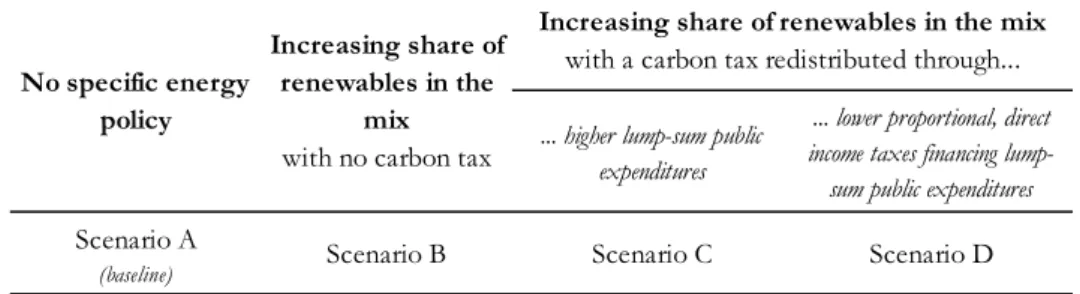
We define 4 policy scenarios. Scenario A is a no-reform scenario in the energy sector. The share of renewables in electricity is frozen in the future to its latest known level and no carbon tax is implemented. Scenario B introduces a rise of renewables10 from the current levels to 35% of the
production of electricity in 2020, 50% in 2030 and 65% in 2040. This corresponds to the target publicly set by German authorities. In the model, this weighs on wholesale electricity prices but bolsters network costs, feed-in tariffs and retail prices. Scenario C adds to scenario B the implemen-tation of a carbon tax from 2015 onwards. In the model, the rate of the carbon tax begins at 32€/t in 2015, increases by 5% in real terms per year, until reaching a cap of 98€/t in 2038 and remains constant afterwards.11 The income associated with the carbon tax is fully redistributed to private
agents through higher lump-sum public expenditures. Eventually, scenario D differs from scenario C only insofar as the income of the carbon tax is recycled through lowering the proportional, direct tax on income that finances lump-sum public expenditures, with the level of the latter remaining unchanged.
Scenario A is assumed to be the baseline scenario. If governments decides any reform incoporated in scenarios B, C or D, this announcement modifies the informational set of all living agents in 2010. This triggers an optimal reoptimisation process at that year, yielding new future intertemporal paths for consumption, savings and capital supply.
... higher lump-sum public expenditures
... lower proportional, direct income taxes financing lump-sum public expenditures
Scenario A
(baseline) Scenario B Scenario C Scenario D
Increasing share of renewables in the mix
with a carbon tax redistributed through...
No specific energy policy
Increasing share of renewables in the
mix
with no carbon tax
Figure 1: Scenarios simulated in the model
9Additionnally, facilities producing electricity out of nuclear energy (which amount to one fourth of the electricity produced in Germany in the early 2010’s) are shut down in the future in all scenarios - as publicly announced by the German government in the aftermath of the events in Fulushima in 2011.
1 0Defined here as encompassing hydroelectricity, wind and PV; along with renewables substitutes (i.e., biomass, biogas, biofuel, waste).
1 1The price of CO2 in the EU-ETS is supposed to be indexed to the rate of the carbon tax after a few years and increases accordingly in the next decades in the model.
Such a framework allows for measuring the dynamic impacts on growth and intertemporal welfare of each cohorts of a rising share of renewables in the energy mix and a fully recycled carbon tax. By construction, in a dynamic GE model, all the variables interact with one another. The only way to isolate the influence of one variable (i.e., increasing renewables, environmental taxation) on another (i.e., GDP, cohorts’ welfare...) in the intertemporal, general equilibrium consists in running two scenarios where the only difference is the first variable (i.e., increasing renewables, environmental taxation). With this setting, the effects of increasing the share of renewables in the energy mix can be assessed by computing the differences between the results of scenario B and scenario A. The influence of implementing a carbon tax stems from the comparison between scenario C (or D) with scenario B, depending on the assumption as concerns the redistribution of the public income associated with the tax to households. The difference between scenario D and C mirrors the effect of recycling a carbon tax through lower proportional taxes rather than higher lump-sum public expenditures, namely, the so-called "second dividend" on an environmental taxation.
3
Results
Some aggregate results of the scenarios are presented before going in more details to the implications on GDP growth and intergenerational equity.
3.1
Aggregate effects
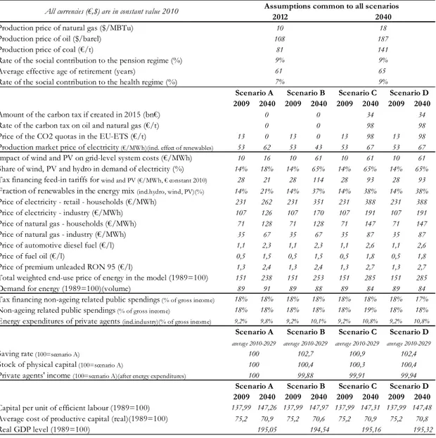
• in the baseline scenario A where no specific energy policy is implemented, the prices of fossil fuels keep increasing over the next decades by assumption. No specific policy bolsters the develop-ment of the production of electricity out of renewables from 2012 on. Accordingly, the amount of the tax financing feed-in tariffs declines gradually in the future to reach 21€/MWh in 2040 (in line with declining costs of production for wind and PV stemming from learning-by-doing productivity effects). Coal firing remains the main peaker on the electricity market in the future (in part because the price of CO2 in the EU-ETS is assumed to remain depressed in this scenario). The rise in the prices of fossil fuels on world markets triggers an upward trend in the total weighted end-use price of energy (+58% in real terms from 2009 to 2040). In this context, the total demand for energy almost stabilises while the activity keeps growing. The rise of total renewables12 in the energy mix (from
14% of total demand of energy in 2009 to 21% in 2040) mirrors the consequences on the energy mix of the surge in the prices of fossil fuels. The capital per unit of efficient labour in Germany rises gradually over the future decade since German demography is ageing relatively quickly and will keep weighing on the labour force. Accordingly, the future cost of productive capital declines in the model.
• in scenario B (which differs from scenario A only insofar as public authorities set higher quantitative targets for the future development of renewables), the energy policy implies a rise of renewables13 as a share in the production of electricity from the current levels to 35% in 2020, 50%
1 2Total renewables are defined here as encompassing hydroelectricity, wind, PV, biomass, biofuels, biogas, waste. 1 3Renewables in the electricity sector are defined here as encompassing hydroelectricity, wind and PV .
in 2030 and 65% in 2040 - as publicly announced by German authorities. PV, onshore and offshore wind produce overall 157TWh in 2020 in the model14, entailing a downward effect on wholesale
prices of -27€/MWh in 2040. The associated consequences are sizeable for feed-in tariffs (surging from 37€/MWh in 2013 to 114€/MWh in 2040) as well as for electric network costs (with an upcard specific effect of 10€/MWh in 2009 and 61€/MWh in 2040). The average retail price of electricity for industry rises by 59% in 2040 in real terms as compared to its level in 2009 (corresponding to 180% rise in nominal terms over the same period)15. The total weighted end-use price of energy
surges from 2009 to 2040 (+67% in real terms). The share of total renewables (i.e., biomass, biofuels, biogas, hydro, wind and PV) in the total final consumption of energy reaches 37% in 2040. The total demand for energy is lower in scenario B than in scenario A because prices of energy are higher.
• Scenario C differs from scenario B only insofar as public authorities implement a carbon tax from 2015 on, fully recycling it with higher lump-sum public expenditures. Retail prices of electricity for industry rise by 78% in 2040 in real terms as compared to their level in 2009. The total weighted end-use price of energy displays a strong upward trend (+88% in real terms from 2009 to 2040). In this context, the total demand for energy declines by -6% in volume over the next decades.16 Taxation of carbon magnifies the effects on energy demand stemming from high
prices of fossil fuels on markets, along with the impact of the development of renewables. However, the share of total renewables17 in the total final consumption of energy is 38% in 2040: this result,
compared to its counterpart in scenario B (i.e., 37%) suggests that the impact on the energy mix of this carbon tax remains limited in the model. Sensitivity analysis indeed confirms that the prices of fossil fuels on world markets or centralised development of renewables with quantitative targets set by policy planners have more influence on the energy mix than implementing a carbon tax with a rate less than 100€/t. As concerns public finances, the revenue associated with the carbon tax modeled here (23bn€2010 in 2030 and 34bn€2010 in 2040) is redistributed to the households each
year from 2015 on, through higher lump-sum public expenditures. In 2040, these lump-sum public expenditures are 1,1 point of percentage (of private agents’ income) higher than in scenarios A and B with no carbon tax.
• Scenario D differs from scenario C only insofar as the revenue of the carbon tax is fully redistributed to the private agents by lowering the proportional, direct tax financing the lump-sum public expenditures regime (with unchanged non-ageing public spending). In 2040, this proportional income tax is 1,1 point of percentage (of private agents’ income) lower than in scenarios A, B and C.
1 4This is close to the German official target of 146TWh, which does not take account of GE effects (whereas the model does).
1 5Assuming an annual rate of inflation of 1,5%.
1 6By assumption, energy efficiency gains are constant in the model. Had they accelerated, the decline of energy demand would have been stronger. The assumption of stable annual energy gains has no significant impact of the results as the results are presented as differences between policy scenarios that rely on the same assumptions as regards energy efficiency.
Production price of natural gas ($/MBTu) Production price of oil ($/barel) Production price of coal (€/t)
Rate of the social contribution to the pension regime (%) Average effective age of retirement (years)
Rate of the social contribution to the health regime (%)
2009 2040 2009 2040 2009 2040 2009 2040
Amount of the carbon tax if created in 2015 (bn€) 0 0 34 34
Rate of the carbon tax on oil and natural gas (€/t) 0 0 98 98
Price of the CO2 quotas in the EU-ETS (€/t) 13 0 13 0 13 98 13 98
Production market price of electricity (€/MWh)(incl. effect of renewables) 53 62 53 43 53 67 53 67
Impact of wind and PV on grid-level system costs (€/MWh) 10 16 10 61 10 61 10 61
Share of wind, PV and hydro in demand of electricity (%) 14% 18% 14% 65% 14% 65% 14% 65%
Tax financing feed-in tariffs for wind and PV (€/MWh, € constant 2010) 28 21 28 114 28 93 28 93
Fraction of renewables in the energy mix (incl.hydro, wind, PV)(%) 14% 21% 14% 37% 14% 38% 14% 38%
Price of electricity - retail - households (€/MWh) 231 262 231 351 231 388 231 388
Price of electricity - industry (€/MWh) 107 126 107 170 107 191 107 191
Price of natural gas - households (€/MWh) 71 128 71 128 71 147 71 147
Price of natural gas - industry (€/MWh) 35 67 35 67 35 87 35 87
Price of automotive diesel fuel (€/l) 1,1 2,3 1,1 2,3 1,1 2,6 1,1 2,6
Price of fuel oil (€/l) 0,5 1,5 0,5 1,5 0,5 1,8 0,5 1,8
Price of premium unleaded RON 95 (€/l) 1,3 2,4 1,3 2,4 1,3 2,7 1,3 2,7
Total weighted end-use price of energy in the model (1989=100) 151 238 151 253 151 285 151 285
Demand for energy (1989=100)(volume) 89 91 89 88 89 84 89 84
Tax financing non-ageing related public spendings (% of gross income) 18% 18% 18% 18% 18% 18% 18% 17%
Non-ageing related public spendings (% of gross income) 18% 18% 18% 18% 18% 19% 18% 18%
Energy expenditures of private agents (incl.industry)(% of gross income) 9,2% 9,8% 9,2% 10,1% 9,2% 10,8% 9,2% 10,8%
Saving rate (100=scenario A)
Stock of physical capital (100=scenario A)
Private agents' income (100=scenario A)(after energy expenditures)
2009 2040 2009 2040 2009 2040 2009 2040
Capital per unit of efficient labour (1989=100) 137,99 147,26 137,99 147,97 137,99 147,31 137,99 147,48
Average cost of productive capital (real)(1989=100) 75,2 70,9 75,2 70,6 75,2 70,9 75,2 70,8
Real GDP level (1989=100) 195,05 194,54 195,16 195,32
61 65
7% 9%
All currencies (€,$) are in constant value 2010
Scenario A Scenario B Scenario C Scenario D Assumptions common to all scenarios
18 187 141 2012 2040 10 108 81 9% 9%
Scenario A Scenario B Scenario C Scenario D
average 2010-2029 average 2010-2029 average 2010-2029 average 2010-2029
100 100 100 102,7 99,88 Scenario A Scenario B 100,9 102,4 100,4 100,3 100,4 99,91 99,94 Scenario C Scenario D
-0,4% -0,3% -0,2% -0,1% 0,0% 0,1% 0,2% 0,3% 0,4% 0,5% 0,6% 2000 2005 2010 2015 2020 2025 2030 2035 2040 2045 2050
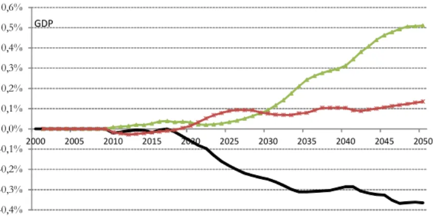
Impact on GDP of increasing the share of renewables in the energy mix (scenario B - scenario A) Impact on GDP of implementing a fully recycled carbon tax (scenario C - scenario B) Impact on GDP of recycling the carbon tax through lower proportional taxes rather than higher lump-sum expenditures (scenario D - scenario C)
GDP
Figure 3: Impact on the level of GDP in the long run of the scenarios simulated in the model
3.2
Implications on growth dynamics
Figure 3 displays the results obtained in the model as concerns growth dynamics. Several results emerge.18
Result 1: Higher quantitative targets set by public authorities for the future development of renewables weigh on economic growth in the long run. This stems from a direct comparison between the results of scenario B and scenario A. Intuitively, the rise in the share of renewables in the energy mix fosters average energy prices for private agents, forcing them to buy at a higher price a good that is necessary for production and has no perfect substitute.
While lessening the demand for energy, the rise of renewables in the energy mix also fosters the stocks of capital and labour. In the private agents’ accounts, higher energy prices stemming from a development of renewables weigh on disposable income. Life-cycle optimizing behaviour imply a rise in the saving rate, entailing an upward effect on the supply of capital. The dynamics of the labour supply and of the optimal average working time is also influenced by the rise in renewables. The first order intratemporal condition for a working individual can be written as 1−ℓ∗
t,a=
c∗
t,a(κξH−1a )
[wtεa(1−τt,D−τt,P−τt,H−τt,NA)+dt,NA−dt,energy]ξ (where 1−ℓ
∗
t,ais optimal leisure and ξ > 0).
Increasing prices of energy bolsters the amount of expenditures in energy (dt,energy) and thus tend
to increase optimal working time. This latter effect remains quantitatively subdued, however. In 1 8In Figure 3, the GDP appears somewhat different in the early 2010’s in the scenarios with a recycling of the carbon tax than in the baseline scenario A, while the carbon tax is assumed to be implemented in 2015 in the model. This mirrors different modelling assumptions that do not have far reaching economic significance nor implications. By assumption, the reform consisting in implementing a carbon tax is announced in 2010 and implemented in 2015 in the model. This triggers reoptimisation in 2010 by forward-looking agents, which account for some small effects right from the beginning of the 2010’s.
the end, higher energy prices stemming from a development of renewables increase the capital per unit of efficient labour. This rise in the stock of capital per capita flows from the private agents’ optimal responses to a negative supply shock that lessens economic output because of increasing prices of energy.19 The existence of retired cohorts which consume relatively more energy, feeds the
downward effect on average income after energy expenditures and the impact on saving. Accordingly, the older the population, the stronger the capital deepening associated with a rise in renewables in the energy mix.
Result 2: a carbon tax, if it is fully recycled, has a positive influence on GDP in the long run. This stems from a direct comparison between the results of scenario C (or D) and scenario B.
This favourable influence on activity in the long run of a fully recycled carbon tax is related to its downward effect on the demand for energy in volume. Indeed, since the carbon tax weighs on the total demand for energy in volume, the rise in the total energy expenditures paid by private agents - which mirrors volume and real price effects altogether - is less than the amount of the carbon tax collected and fully redistributed. Accordingly, the households’ income, which encompasses energy expenditures and public spending, rises in the model. This fosters consumption. Such an effect dominates the upward influence on savings that flows from higher energy prices ceteris paribus. Accordingly, capital supply is lower in scenario C than in scenario B. Labour supply remains quantitatively little affected. Overall, capital per unit of efficient labour is lower when a fully recycled carbon tax is implemented.
The existence of retired cohorts consuming relatively more energy lessens the upward effect on income after energy expenditures and the downward impact on saving. Accordingly, the older the population, the smaller the upward impact on growth (as shown in Figure 3 during the 2010’s and the 2020’s for scenario C) and the smaller the downward impact on the stock of capital associated with the implementation of a fully recycled carbon tax.20
Result 3: Recycling the revenue associated with the carbon tax with lower direct taxes entails more favourable effects on growth than recycling the tax with a rise in lump-sum public spending (i.e., the second dividend is positive in the model). This stems from a direct comparison between the results of scenario D and scenario C. Intuitively, lessening distortionary taxes has a more favourable effect on activity than raising lump-sum public transfers. This is in line with the theoretical litterature on optimal environmental taxation (Nichols (1984), Terkla (1984), Pearce (1991) and Poterba (1991)) which suggests that substituting environmental taxes with other, direct taxes may reduce the distortionary cost of the tax system.
This result mirrors a joint influence of fiscal policy on the households’ income and their life-cycle consumption/saving behaviour, entailing some additional capital deepening when taxes are lowered. In scenario D, lessening the proportional tax amounts, in absolute terms, to distributing more revenues to cohorts receiving higher wages. These cohorts receiving on average a higher gross labour income are relatively older working cohorts, which are more productive in the model than 1 9Only skyrocketting prices for fossil fuels on world markets might influence significantly this result. It could then happen that a higher share of renewables in the energy mix would alleviate tensions on the dynamics of the average prices of energy. This provides with a rationale for a possible positive effect on GDP of the development of renewables - however, only in the very long run, given the amount of remaining reserves of fossil fuels (natural gas, coal).
2 0This can be checked for instance with sensitivity analysis where there is no relation between the level of con-sumption of energy and the age of the private agents.
the younger working cohorts. In line with the life-cycle theory, the saving rate of aged working cohorts is also higher than the one of younger working cohorts. Overall, capital supply is higher in scenario D than in scenario C.
Result 4: the macroeconomic magnitude of the effects on growth obtained in results 1, 2 and 3 remain subdued in the long run.
Around 2050, the macroeconomic magnitude of these effects are close to +/-0,5% of the level of the GDP. This is in line with the "elephant and rabbit" tale in energy economics (Hogan and Manne, 1977) according to which the size of the energy sector in the economy bares it to entail very sizeable effects on growth. This is also globally in line with Knopf et al. (2010) who suggest that meeting environmental objectives so as to mitigate the climate change would trigger only limited macroeconomic long-run costs.
3.3
Intergenerational redistributive effects
3.3.1 Effects on future annual welfare of each cohort
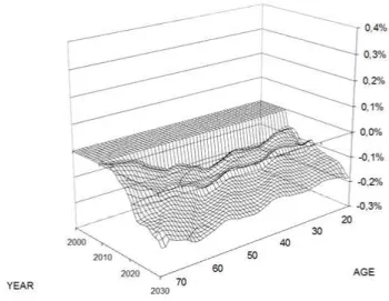
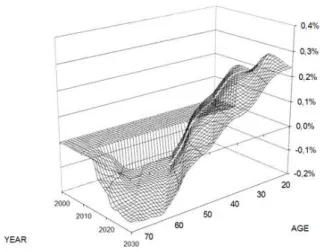
A first detailed analysis of the cohorts loosing or gaining in different scenarios is possible using Lexis surfaces (Figures 4, 5 and 6). A Lexis surface represents in 3 dimensions the level of a variable associated with a cohort of a given age at a given year. The variable considered here is the gain (or loss) of annual welfare of a cohort aged a in a given year t and in a scenario where the carbon tax is recycled through lower proportional income tax compared to the baseline scenario where the carbon tax is recycled through higher lump-sum public spending. Annual welfare refers here to the instantaneous utility function of a private agent in the model, and thus depends on the level of consumption and optimal leisure. Before the announcement of a reform package in 2010, annual current welfare of one cohort is by assumption equal between the vaseline scenario A and any of the reform scenarios considered here. Graphically, this involves a flat portion in the Lexis surface, at value 0. From 2010 onwards, the deformations of the Lexis surfaces mirror the influence of mechanisms of intergenerational redistribution of the reform scenario, as measured by its influence on current welfare.
Result 5: Higher quantitative targets set by public authorities for the future development of renewables trigger intergenerational redistributive effects in the population.
Figure 5 displays the Lexis surface for current annual welfare, at each year and for each cohort in the model, in scenario B as compared to scenario A. Accordingly it materializes the intergenerational effects of setting higher quantitative targets for the future development of renewables. It may be useful to remind here that annual welfare in the model depends on the optimal consumption and leisure paths defined by perfectly anticipating households over their whole life-cycle, and not only on their current income.
As shown in Figure 5, higher quantitative targets set by public authorities for the development of renewables weighs on the future annual welfare of all cohorts. However, the detrimental effect in the short run is slightly less pronounced for currently retired generations. This flows mainly from the joint influence of a permanent income effect and of an energy consumption effect:
• the permanent income effect is intuitive. The shorter the period of remaining life, the smaller the effect on optimal behaviours, defined on an intertemporal basis, stemming from a permanent rise in energy prices and the development of renewables. Thus the currently older the cohort, the smaller the detrimental effect on its permanent income associated with a rise of renewables.
• the energy consumption effect is mechanical. Since the energy consumption increases with age, the detrimental impact of rising energy prices concentrates relatively more on older households. The energy consumption effect thus partially offsets the permanent income effect. Figure 5 provides with the net influence of both mechanisms on future current welfare.
Result 6: A carbon tax, if fully recycled, has pro-youth intergenerational redistributive proper-ties.
Figure 6 displays the Lexis surface for current annual welfare, at each year and for each cohort in the model, in scenario C as compared to scenario B. Accordingly it materializes the intergenerational effects of implementing a fully recycled carbon tax. Two mechanisms are involved. Both favor younger and future cohorts:
• a permanent income effect: the shorter the period of remaining life, the smaller the favourable effect on optimal behaviours, defined intertemporally, of a permanent rise in lump-sum public expenditures. Thus the currently older the cohort, the smaller the positive influence on permanent income associated with the recycling of the carbon tax.
• an energy consumption effect: since the energy consumption increases with age, the mag-nifying effect of a carbon tax on energy prices weighs more on older households.
The net effect of recycling a carbon tax is thus negative for the older generations, as shown in Figure 6, because the detrimental energy consumption effect (which is relatively stronger for them) dominates the favourable permanent effect (which is relatively smaller for these generations). For young and future cohorts, the detrimental energy consumption effect (which is relatively subdued as far as they are concerned) is dominated by the favourable permanent effect (which is relatively stronger for these generations).
Result 7: Recycling a carbon tax through lower direct, proportional taxes rather than higher lump-sum public expenditures conveys specific redistributive effects that benefit to young and future generations.
Figure 7 displays the Lexis surface for current annual welfare, at each year and for each cohort in the model, in scenario D as compared to scenario C. Accordingly it materializes the intergenerational effects of the second dividend associated with the carbon tax. One main mechanism is involved here and it relatively favours young and/or active generations. The capital per unit of efficient labour is higher when the carbon tax is recycled through lower proportional taxes (as in scenario D) rather than through higher public lump-sum expenditures (as in scenario C) - as seen in table 2 and explained in result 3. This weighs on the yield of the saving of these cohorts which have accumulated significantly more capital than younger cohorts when the carbon tax is implemented in the model. This weighs relatively more on the optimal consumption path of older cohorts in the
Figure 4: Effect on annual welfare of increasing the share of renewables in the energy mix (%, Germany) (scenario B - scenario A)
Figure 5: Effect on annual welfare of implementing a carbon tax fully recycled through higher lump-sum public expenditures (%, Germany) (scenario C - scenario B)
Figure 6: Effect on annual welfare of implementing a carbon tax fully recycled through lower proportional taxes on income rather than higher lump-sum public expenditures (%, Germany) (scenario D - scenario C)
model.21
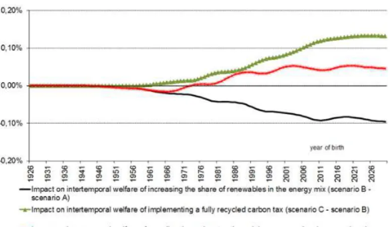
3.3.2 Effects on intertemporal welfare of private agents
Computing the intertemporal welfare of each cohort over its whole lifetime allows for precising and completing the above analysis of intergenerational redistributive effects. Figure 7 displays the effects on intertemporal welfare for each scenario of reform.
Result 8: a higher share of renewables in the energy mix weighs relatively more on the in-tertemporal welfare of young and future generations. As long as inin-tertemporal welfare is defined as depending only on consumption and leisure, all cohorts would suffer a loss of wellbeing in case of a rising share of renewables in the energy mix. However, the younger a cohort today, the longer it will bear the cost of higher energy prices associated with the development of renewables in the mix, ceteris paribus, the higher the detrimental influence on its intertemporal welfare. This result is relatively robust to realistic hypothesis about future world energy prices.
Result 9: A fiscal policy implementing a fully recycled carbon tax may more than offset the detrimental effects of increasing renewables on private agent’s intertemporal welfare, and would display pro-youth redistributive features. This result holds especially if the carbon tax is recycled through lower proportional taxes on income rather than higher public lump-sum expenditures.
2 1These intergenerational redistributive effects are robust to different assumptions as concerns future prices of fossil fuels on world market. The Lexis surfaces obtained in scenarios with low prices of fossil fuels on world markets display the same patterns as those presented in the text.
Figure 7: Effects on the intertemporal welfare of scenarios simulated in the model (%)
4
Conclusion and policy implications
This paper assesses the respective effects on growth and intertemporal welfare of a rising share of renewables in the energy mix and of a fully recycled carbon tax. The main result is that while both policies foster the average price of energy, they entail opposite (though limited) impacts on growth and intertemporal welfare of the cohorts. The intuition is that the recycling of a carbon tax fosters consumption and labour supply, and thus growth and welfare, whereas an increasing share of renewables does not. Results also suggest that a higher share of renewables and a recycled carbon tax trigger intergenerational redistributive effects, with the former being relatively detrimental to young generations and the latter being more pro-youth.
The policy implication of this article is not that implementing a fully recycled carbon tax should be preferred to setting higher quantitative targets for renewables in the future energy mix. Rather, it implies that significant economic gains arise when both are implemented. The model shows that the price-signal associated with a carbon tax (with a rate less than 100€/t) triggers relatively contained effects on the structure of the energy mix. In this context, a policy aiming at modifying the energy mix while simultaneaoulsy achieving some form of neutrality as concerns the GDP and triggering some pro-youth intergenerational equity could usefully contemplate implementing simultaneously higher quantitative targets for the future development of renewables and a carbon tax fully recycled through lower proportional taxes.
A
Description of the GE-OLG model
This CGE model displays an endogenously generated GDP with exogenous energy prices influ-encing macroeconomic dynamics, which in turn affect the level of total energy demand and the future energy mix. GE-OLG models combine in a single framework the main features of GE models (Arrow and Debreu, 1954), Solow-type growth models (Solow, 1956), life-cycle models (Modigliani and Brumberg, 1964) and OLG models (Samuelson, 1958). The development of applied GE-OLG models, using empirical data, owes much to Auerbach and Kotlikoff (1987). This GE model includes a detailed overlapping generations framework so as to analyse, in a dynamic setting, the intergen-erational redistributive effects of energy and fiscal reforms, and to take account of demographic dynamics on the economic equilibrium.22
A.1
The Energy sector
A.1.1 Energy prices
End-use prices of natural gas, oil products and coal (q1,t, q2,t, q3,t) The end-use prices of
natural gas, oil products and coal (qi,t, i ∈ {1; 2; 3}) are computed as weighted averages of prices of
different sub-categories of energy products: ∀i ∈ {1; 2; 3} , qi,t= n j=1
ai,j,tqi,j,t. qi,j,t stands for the
real price of the product j of energy i at year t. For natural gas (i = 1), two sub-categories j are modeled: the end-use price of natural gas for households (j = 1) and the end-use price of natural gas for industry (j = 2). For oil products (i = 2), three sub-categories j are modeled: the end-use price of automotive diesel fuel (j = 1), the end-use price of light fuel oil (j = 2) and the end-use price of premium unleaded 95 RON (j = 3). For coal (i = 3), two sub-categories j are modeled: the end-use price of steam coal (j = 1) and the end-use price of coking coal (j = 2). This hierarchy of energy products covers a great part of the energy demand for fossil fuels. The ai,j,t’s weighting
coefficients are computed using observable data of demand for past periods. For future periods, they are frozen to their level in the latest published data available: whereas the model takes account of interfuel substitution effects (cf. infra), it does not model possible substitution effects between sub-categories of energy products (for which data about elasticities are not easily available).
The end-use prices of sub-categories of natural gas, oil or coal products (qi,j,t) are in turn
computed by summing a real supply price with transport/distribution/refining costs and taxes: ∀i ∈ {1; 2; 3} , ∀j, qi,j,t= qi,j,t,s+ qi,j,t,c+ qi,j,t,τ
2 2In line with most of the literature on dynamic GE-OLG models, the model used here does not account explicitly for effects stemming from the external side of the economy. First, the question that is adressed here is: what optimal choice should the social planner do as concerns energy and fiscal transition so as to maximize long-run growth and minimize intergenerational redistributive effects? Accounting for external linkages would not modify substantially the answer to this question. It would smooth the dynamics of the variables but only to a limited extent. Home bias (the “Feldstein-Horioka puzzle”), exchange rate risks, financial systemic risk and the fact that many countries in the world are also ageing and thus competing for the same limited pool of capital all suggest that the possible overestimation of the impact of ageing on capital markets due to the closed economy assumption is small.
• qi,j,t,s stands for the real supply price at year t of the product j of energy i. This real
price is computed as a weighted average of real import costs and real production prices: ∀i ∈ {1; 2; 3} , ∀j, qi,j,t,s = [Mi,j,tmi,j,t+ Pi,j,tpi,j,t] / [Mi,j,t+ Pi,j,t] where Mi,j,t stands for imports in
volume of the product j of energy i at year t ; mi,j,t stands for imports costs of the product j of
energy i at year t ; Pi,j,t stands for national production, in volume, of the product j of energy i
at year t ; pi,j,t stands for production costs of national production of the product j of energy i at
year t. The weights Mi,j,t and Pi,j,t are computed using OECD/IEA databases for past periods,
and frozen to their latest known level for future periods.
• qi,j,t,c stands for the cost of transport and distribution and/or refinery for the different
energy products for natural gas, oil and coal. More precisely, q1,1,t,c stands for the cost of transport
and distribution of natural gas for households in year t; q1,2,t,c stands for the cost of transport
of natural gas for industry in year t; q2,1,t,c , q2,2,t,c and q2,3,t,c stand respectively for the cost of
refining and distribution for automotive diesel fuel, light fuel oil and premium unleaded 95 RON in year t; q3,1,t,cand q3,2,t,c stand respectively for the transport cost of steam coal and coking in year
t. The qi,j,t,c’s are calculated as the difference between the observed end-use prices excluding taxes
by category of products (as provided by OECD/IEA databases) and the supply prices (the qi,j,t,s’s)
as computed above. For future periods, each qi,j,t,c’s is computed as a moving average over the 10
preceding years before year t.
• qi,j,t,τ stands for the amount, in real terms, of taxes paid by an end-user of a product j of
energy i at year t. For past periods, these data are provided by OECD/IEA databases. They include VAT, excise taxes, and other taxes: qi,j,t,τ = V ATi,j,t+ Excisi,j,t+ othersi,j,t+ carbon taxi,j,t. For
future periods, the rate of V ATi,j,tand othersi,j,tare computed as a moving average over the latest
10 years before year t, and the absolute real level of Excisi,j,tis computed as a moving average over
the latest 10 years before year t. For future periods, depending on the reform scenario considered, qi,j,t,τ can also include a carbon tax (carbon taxi,j,t) which is computed by applying a tax rate to
the carbon contained in one unit of volume of product j of energy i.
Prices of electricity (q4,t) The real end-use price of electricity is computed as a weighted average
of prices of electricity for households and industry (i = 4); q4,t= 2 j=1
a4,j,tq4,j,t. q4,j,tstands for the
end-use real price, at year t , of the product j of electricity. Two sub-categories j are modeled: the end-use price of electricity for households (j = 1) and the end-use price of electricity for industry (j = 2). The a4,j,t’s weighting coefficients are computed using observable data of demand for past
periods, and frozen to their level in the latest published data available for future periods. Real end-use prices of electricity are computed by adding network costs of transport and distribution (q4,j,t,c)
and differents taxes (VAT, excise, tax financing feed-in tariffs for renewables, carbon tax...)(q4,j,t,τ)
to an endogenously generated (structural) wholesale market price of production of electricity (q4,t,s):
(i = 4); ∀j, q4,j,t= q4,t,s+ q4,j,t,c+ q4,j,t,τ
Wholesale structural market price of production of electricity (q4,t,s) The wholesale
market price of production of electricity (q4,t,s) is computed from an endogenous average peak price
of electricity and a peak/offpeak spread: ∀j, q4,t,s= (qel,peak,t+spread2peak,t∗qel,peak,t). The parameter
The peak market price of production of electricity (qel,peak,t) derives from costs of production of
electricity among different technologies, weighted by the rates of marginality in the electric system of each production technology: qel,peak,t =
9 x=1
ξel,x,t̺el,x,t,prod (1+ξel,import,t) 9
x=1ξel,x,t +ξel,import,t+̟f atal,t
. The costs of producing electricity (̺el,x,t,prod) are computed for 9 different technologies x: coal (x = 1), natural gas (x = 2), oil (x = 3), nuclear (x = 4), hydroelectricity (x = 5), onshore wind (x = 6), offshore wind (x = 7), solar photovoltaïc (x = 8), and biomass (x = 9). The ξel,x,t’s stand for the rates of marginality in the electric system of the producer of electricity using technology x
Cost of production of electricity among different technologies (̺el,x,t,prod) Following, for instance, Magné, Kypreos and Turton (2010), each ̺el,x,t,prodis computed as the sum of variable costs (i.e., fuel costs and operational costs) and fixed (i.e., investment) costs of producing electricity: ∀x, ̺el,x,t,prod= ̺el,x,t,f uel+̺co2 price,t∗̺el,x,t,co2em
̺el,x,t,therm + ̺el,x,t,ops +̺el,x,t,f ixedwhere ̺el,x,t,f uelstands
for the fuel costs for technology x (either coal, oil, natural gas, uranium, water, biomass for costly fuel, or wind and sun for costless fuels) measured in €/MWh; ̺el,x,t,therm stands for thermal efficiency (in %). CO2 costs are measured by the exogenous price of CO2 on the market for quotas (EU ETS) (̺co2 price,t, in €/ton), as applied to technology x characterised by an emission factor ̺el,x,t,co2em expressed in t/MWh; ̺el,x,t,opsstands for operational and maintenance variable costs (in €/MWh). Fixed costs ̺el,x,t,f ixed are expressed in €/MWh and computed according to the following annuity formula: ∀x, ̺el,x,t,f ixed = ̺el,x,t,inv
1+̺el,x,t,prodloss
1+̺el,x,t,learning̺el,x,t,cap c
(1−(1+̺el,x,t,cap c)−̺el,x,t,lif e)̺el,x,t,util
. ̺el,x,t,inv corresponds to overnight cost of investment (expressed in €/MW); ̺el,4,t,prodloss is the rate of productivity loss due to increased safety in the nuclear industry ; ̺el,x,t,learning is the learning rate for renewables; ̺el,x,t,cap c stands for the cost of capital (̺el,x,t,cap c= 10%); ̺el,x,t,lif e the average lifetime of the facility (in years) depending of the technology used; ̺el,x,t,util the utilisation rate of the facility (in hours). All these parameters are exogenous and found mainly in IEA and/or NEA databases.
Rates of marginality (ξel,x,t) and main peaker between coal firing and natural gas firing (ξel,1,t and ξel,2,t) The rates of marginality are the fraction of the year during which a producer of electricity is the marginal producer, thus determining the market price during this period. These rates are exogenous in the model. They are computed in France by the French Energy Regulation Authority and/or by operators in the electric sector in France and Germany. For future periods, the model uses the 2010 values which are frozen onwards.23
The computation of the future values for ξel,1,tand ξel,2,tin the model stems from an endogenous determination of the main peaker, either coal firing or natural gas firing. The model computes, for each year t > 2012, the clean dark spread and the clean dark spread. These are mainly influenced by CO2 prices (̺co2 price,t), respective emission factors (̺co2 price,tand ̺el,2,t,co2em) and fuel costs (̺el,x,1,f uel and ̺el,x,2,f uel). Each year t > 2012, if the difference between the clean spark spread 2 3Accordingly, the formula used for computing (qelec,peak,t) assumes that the energy mix of imports is the same as the domestic energy mix.
and the clean dark spread is negative, and if the clean dark spread alone is positive, then the main peaker is coal. The reverse holds if signs are opposite (the natural gas become main peaker).
Simulated market peak price of production of electricity (qel,peak,t) The development
of fatal producers of electricity (onshore wind, offshore wind and solar PV) weighs down on market prices by moving rightward the supply curve. We take account of this phenomenon by introducing a parameter ̟f atal,t 24 in the denominator of the expression of qel,peak,twhich allows for capturing
some characteristics of fatal producers of electricity. Their marginal cost is nil and they are not marginal producers: hence ξel,6,t = ξel,7,t = ξel,8,t = 0% in the numerator. They shift the supply curve of the wholesale market rightward: hence the more they produce, the less the market price. This is taken into account in the model by introducing ̟fatal,t at the denominator of qel,peak,t. We
assume that the mark-up of market price of electricity over the average weighted cost of production is zero. A parameter markupel,tcould have been included. Including such a parameter would have
brought about the question of the modelling of the associated surplus between economic agents. Since this parameter would have remained constant, its first order effect on the dynamics of the model would have been zero.
Network costs of electricity (q4,j,t,c) q4,j,t,c stands for the cost of transport and/or
dis-tribution of electricity. More precisely, q4,1,t,c stands for the cost of transport and distribution of
electricity for households in year t; q4,2,t,c stands for the cost of transport (only) of electricity for
industry in year t. The q4,j,t,c’s are calculated as the difference between the observed end-use prices
excluding taxes of electricity for households or industry (as provided by OECD/IEA databases) and the supply price (q4,t,s) as computed above. For future periods, each q4,j,t,c’s is computed as a
moving average over the 10 preceding years before year t. In scenarios of reforms involving a rise in the fraction of electricity produced out of fatal producers (i.e., onshore and offshore wind and solar PV), supplementary network costs are incorporated in the model following NEA (2012) orders of magnitude.25
Taxes on electricity (q4,j,t,τ): VAT, excise tax, tax financing feed-in tariffs for
re-newables q4,j,t,τ stands for the amount, in real terms, of taxes paid by an end-user of
elec-tricity (either households (j = 1) or industry ( j = 2)) at year t: ∀j ∈ {1; 2} , q4,j,t,τ =
V AT4,j,t+ Excis4,j,t+ others4,j,t+ T afF T AR4,t. For past periods, these data are provided by
OECD/IEA databases. They include VAT, excise taxes and other taxes. For future periods, the rates of V AT4,j,tand others4,j,t are computed as a moving average over the latest 10 years before
year t, and the absolute real level of Excis4,j,t (if any) is computed as a moving average over the
latest 10 years before year t. For future periods, depending on scenario reforms, q4,j,t,τ can also
include a tax financing feed-in tariffs for fatal producers of electricity (T af F T AR4,t, in €/MWh).
Indeed, government in the model is assumed, when it decides to implement an energy transition, to create a scheme compensating the difference between the market price of electricity (q4,j,t,s) and
2 4̟f atal,tassesses the penetration level of fatal producers of electricity at year t and is computed as the ratio between production of electricity out of wind and solar PV (x ∈ {6; 7; 8}, in GWh) in year t divided by total demand of electricity in year t − 1.
2 5NEA (2012) computes the supplementary network cost (in €/MWh) of a given rise in the penetration rate of intermittent sources of electricity.