Computational imaging with scattered photons to see inside the body

Computational Imaging with Scattered Photons to

See inside the Body

by

Tomohiro Maeda

Submitted to the the Program in Media Arts and Sciences,

in partial fulfillment of the requirements for the degree of

Master of Sciencein Media Arts and Sciences

at the

MASSACHUSETTS INSTITUTE OF TECHNOLOGY

June 2020

© Massachusetts Institute of Technology 2020. All rights reserved.

Author . . . .

the Program in Media Arts and Sciences,

May 18, 2020

Certified by. . . .

Ramesh Raskar

Associate Professor

Thesis Supervisor

Accepted by . . . .

Tod Machover

Academic Head, Department Committee on Graduate Theses

Computational Imaging with Scattered Photons to See inside

the Body

by

Tomohiro Maeda

Submitted to the the Program in Media Arts and Sciences, on May 18, 2020, in partial fulfillment of the

requirements for the degree of

Master of Sciencein Media Arts and Sciences

Abstract

Conventional imaging for health applications captures photons from the objects that are directly in the field of view of the camera. In this thesis, we develop computational frameworks to exploit scattered photons to image regions that are not directly visible to the camera.

First, we will explore a new framework to model volumetric scattering with time-of-flight imaging to recover objects in scattering media with less need for calibrations. This technology can be applied to see under the skin. Second, we will exploit fluores-cent tags, and quantum dots to image tagged objects around the corner for endoscopy with traditional cameras. We introduce a novel parametric approach to NLOS imag-ing for localizimag-ing tags around corners from radiometric measurements. The goals of the thesis are to develop novel approaches to model scattered light-transport and to demonstrate recovery of hidden objects, though scattering or around corners. The proposed technology can extend the scope of medical imaging.

Thesis Supervisor: Ramesh Raskar Title: Associate Professor

Computational Imaging with Scattered Photons to See inside the Body by

Tomohiro Maeda

Thesis Advisor. . . . Ramesh Raskar Associate Professor of Media Arts and Sciences MIT Program in Media Arts and Sciences

Thesis Reader . . . . Joseph A. Paradiso Alexander W. Dreyfoos (1954) Professor of Media Arts and Sciences MIT Program in Media Arts and Sciences

Thesis Reader . . . . Edward Boyden Professor of Media Arts and Sciences MIT Program in Media Arts and Sciences

Acknowledgments

I would not have been able to complete this work without the help from many people. First, I would like to thank Prof. Ramesh Raskar for the guidance, support and en-couragement. I learned a lot from Ramesh’s positive, optimistic views for everything. I also would like to thank Prof. Joseph Paradiso and Prof. Edward Boyden for the support and constructive feedback for the work. I thank Prof. Moungi who has been generously supporting me with the equipment necessary for the research.

I am thankful to Achuta Kadambi, who has been supporting me since I started as a UROP camera culture group. He has been a great mentor since the beginning. I thank my colleagues and mentors, Ayush Bhandari, Guy Satat, Tristan Swedish, Praneeth Vepakomma, Lagnojita Sinha, Connor Henley, Subhash Sadhu and Abhishek Singh for the inspirations and friendships.

Finally, I am grateful to my wife, Olena Fedoniuk. She has been next to be for the best and worst time through the Masters program. I would not be able to push myself without her supporting and encouraging me. Olena always reminded me that there is always something good in any moment.

Contents

0.1 Motivation . . . 18

0.1.1 Imaging through volumetric scatterings . . . 18

0.1.2 Imaging Tagged Objects around Corner . . . 19

0.2 Contributions . . . 20

0.2.1 Imaging through volumetric scatterings . . . 20

0.2.2 Imaging Tagged Objects around Corner . . . 21

1 Background and Related Works 25 1.1 Imaging through volumetric scattering . . . 25

1.1.1 Ballistic photon gating . . . 25

1.1.2 Coherent Imaging . . . 26

1.1.3 Computational Light Transport . . . 26

1.2 Imaging around corners . . . 27

1.2.1 ToF-based NLOS imaging . . . 27

1.2.2 Coherence-based NLOS imaging . . . 29

1.2.3 Intensity-based NLOS imaging . . . 30

2 Automatic Differentiation for All Photons Imaging to See inside Volumetric Scattering Media 31 2.1 Forward Model . . . 32

2.2 Reconstruction Algorithm . . . 36

2.2.1 Estimation of optical properties . . . 37

2.2.2 Estimation of target . . . 40

2.3.1 Simulation . . . 41

2.3.2 Experiment . . . 43

2.4 Discussion . . . 48

2.4.1 Practical Limitations . . . 48

2.4.2 Trade off between efficiency, accuracy, and modeling of complex scenes . . . 49

2.4.3 Resolution Analysis . . . 49

2.4.4 Applications . . . 50

2.5 Conclusions and Future Directions . . . 51

3 Imaging tagged objects around corners 53 3.1 Forward Model . . . 54

3.2 Localizing tags around corners . . . 56

3.2.1 Linear model with sparsity assumption . . . 57

3.2.2 Parametric Model . . . 58 3.2.3 Multiple Tags . . . 59 3.3 Validation . . . 60 3.3.1 Synthetic Results . . . 60 3.3.2 Experimental Results . . . 68 3.4 Discussion . . . 70 3.4.1 Limitations . . . 70 3.4.2 Applications . . . 72

3.4.3 Conclusions and Future Directions . . . 73

List of Figures

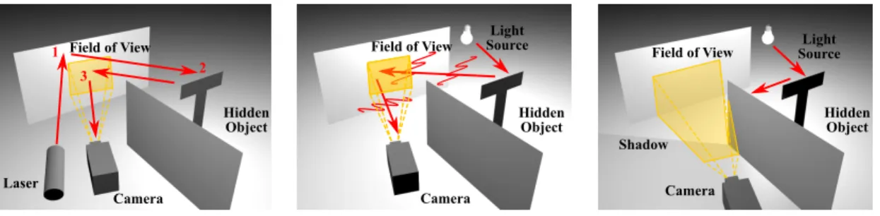
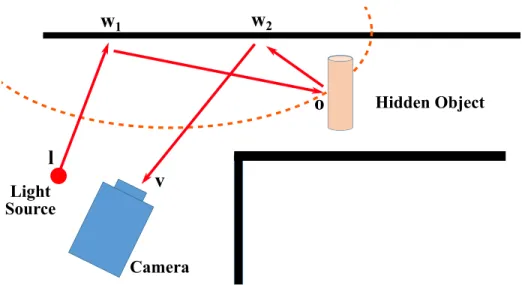
1-1 Summary of NLOS imaging setup for different types of measurement. (a) Time-of-flight based techniques exploit the path length of three bounce photons to constrain the location of the hidden object. (b) Coherence-based techniques exploit speckle patterns or spatial coher-ence, which preserves the information of the hidden scene. (c) Intensity-based information typically exploits occluding geometries, which makes the inverse problem of NLOS imaging less ill-posed. . . 27 1-2 Layouts of NLOS imaging setups with ToF measurement. Photon

emit-ted by the light source at l travels to the hidden surface point w1 (first

bounce), reaches the hidden object surface o (second bounce), and hit the visible surface again at w2 before being captured by the detector

at v. . . 28 2-1 Overview of the imaging setup to see through scattering. Our proposed

technique operates in a transmission-mode setup, where the illumina-tion source (pulsed laser) and the detector (SPAD array) are on the opposite side of the scattering media. A SPAD array captures an ultra-fast measurement of the scattered photons. We computationally model and recover the optical properties and the target in the tissue phantom. 32 2-2 Exploiting automatic differentiation towards imaging to expand the

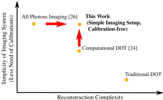
capability of All Photons Imaging. We computationally improve the existing simple imaging system for more complex and realistic scenarios. 33

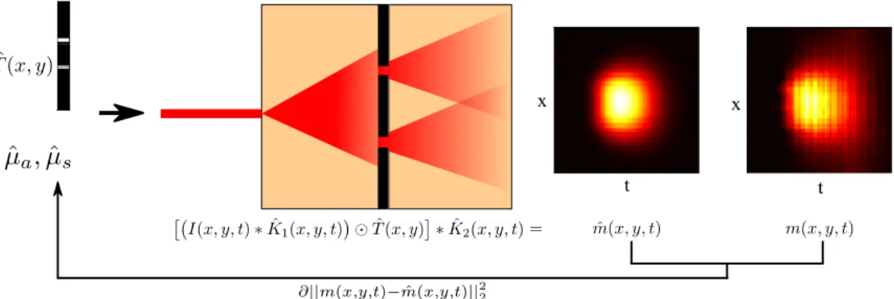
2-3 An overview of the forward model and reconstruction. The forward model is represented as a sequence of 3D convolution with a blur ker-nel 𝐾1(𝑥, 𝑦, 𝑡; 𝐷, 𝑑1), layer-wise Hadamard multiplication with the

tar-get 𝑇 (𝑥, 𝑦), followed by another 3D convolution with a blur kernel 𝐾2(𝑥, 𝑦, 𝑡; 𝐷, 𝑑2). We estimate the optical properties of the

scatter-ing medium by minimizscatter-ing the observed measurement 𝑚(𝑥, 𝑦, 𝑡) and estimated measurement ˆ𝑚(𝑥, 𝑦, 𝑡) via gradient descent. . . 36 2-4 Reconstruction of a 2D target within a scattering medium and the

optical properties of the phantom. (a) A 2D target embedded between two phantoms. (b) When a camera observes the scattered light on the surface of the phantom, the target is blurred in space. (c) The scattered light arrives at different time points so that the measurement is blurred over time. (d) Our method successfully reconstructs the sharp edge of the target. (e) The proposed algorithm recovers the reduced scattering coefficient for various initial estimation. . . 42 2-5 A picture of the experiment setup and biomimetic phantom used as a

scattering media.11 . . . 43 2-6 Reconstruction of the targets between two biomimetic phantoms. (a)

Ground truth shape of the target opening. (b) Time-averaged image of the measurement which is integrated over time. (c) Reconstruction from early-arriving photons. The reconstruction is noisy because the scattering media is thick and dense, and there is almost no ballistic photons. (d) Reconstruction with the proposed algorithm. . . 44 2-7 Reconstruction of the target with different acquisition times. As the

acquisition time shortens, the quality of the time-averaged frame and early-arriving photon frames degrades. Our method is still able to recover the horizontal line of “A” for an acquisition time as short as 150ms. . . 46

2-8 Reconstruction with previously proposed closed-form estimation of the optical properties. The closed-from estimation is susceptible to model mismatch and measurement noise as it does not target the consistency between the estimation and the measurement. . . 47 2-9 Estimated blur kernels for different acquisition time. The proposed

method minimizes the different between the actual measurement and the measurement predicted by the forward model. Therefore, the blur kernel of the scattering medium can be estimated robustly even when the SNR is low due to short acquisition time. . . 47 2-10 Reconstruction of the 2D objects with Tikhonov regularization. The

solution with l2 regularization is blurrier than the solution with l1 and total variation regularization. However, this more general assumption still recovers the feature of the objects such as the horizontal line of “A” character. . . 48 2-11 We evaluate the practical resolution of the method using masks with

two openings separated by a small spacing0. . . 50 3-1 Overview of imaging setup for imaging tagged objects around corners.

A laser illuminate a spot s. The hidden tag at o absorbs and emits light at different wavelengths. A camera observes different points on the wall d1, d2, ..., d𝑚. . . 54

3-2 A scene geometry simulated with Mitsuba Renderer. A point source moves outside of the camera’s field of view. The camera observes the intensity at the visible relay wall. . . 60 3-3 Localizing a point light source around a corner from synthetic

measure-ments with the proposed approach. Our method accurately localizes a point source moving on a grid along x and z directions. . . 61 3-4 Localizing a point source around a corner with different levels of

syn-thetic measurement noise. Our method shows robustness to noisy mea-surements. . . 62

3-5 An example of simulated noisy measurement and the estimated mea-surement from the forward model. Our method recovers noiseless ground truth image from accurate estimation of the hidden point source location. . . 63 3-6 Localization of two point sources around corners with different spacing.

The proposed parametric approach resolves the two sources around cor-ners better than linear inversion approach such as OMP. As expected, as the two points becomes closer, it becomes for the proposed method to resolve two points. Instead, the two points locations are estimated in the middle of two points. . . 65 3-7 Localization of two point sources around corners with different random

positions. This results demonstrates that the proposed approaches can estimate the location of multiple objects around corner with different x, y, z positions. . . 66 3-8 Localization of more than 2 point sources around corners with random

positions. We demonstrate localization of 3 (top), 4 (middle) and 5 hidden point sources. . . 67 3-9 The experimental setup for localizing a single point source. A LED is

placed on a 2-axis translation stage. We moved the source along the x-z grid to validate our localization algorithm. . . 69 3-10 Localization of the hidden source moving along a grid. Left figure

shows the diagram of the entire scene setup, and the right figure shows the more detailed comparison of the estimated location and the ground truth. . . 69 3-11 Localization of two point sources around corners. Our method is able

to reasonably estimate the location of the hidden sources (left and middle). However, when the object is too close, the estimates are not accurate. . . 70

3-12 Localization of a single point source around the corner with two point source assumption. The resulting localization is either two points close to the ground truth location, or one point near the ground truth and another point outside of the range of the interest. . . 71 3-13 Localization of two point sources around the corner with three point

source assumption. Two estimated point converges close to the ground truth, where the third point converges outside of the region of the interest (middle, right). However, such convergence is not guaranteed, and there are cases where localization of two sources fail (left). . . 72

List of Tables

1 We consider two cases of computational imaging with scattered photons in this thesis. . . 19 3.1 The localization errors with varying levels of the synthetic noise added

to the rendered measurement. The error is computed as an average of localization of a point source at each grid location defined as shown in Fig. 3-4. The errors are further averaged by running localization with random noises 1000 times. . . 62

Conventional imaging systems capture photons that travel directly from the ob-ject to the detector. A point in the scene can be mapped to a pixel of the camera such that the acquired images immediately reveal the shape and reflectance of the objects. Conventional imaging has limited capabilities to image inside the body. For example, X-ray imaging uses ionizing radiation, which can be harmful to the body. Current endoscopy is limited to see line-of-sight of the camera, and doctors need to carefully manipulate it, which can lead to longer measurement time and potential missing regions. In this thesis, we explore the technologies to use scattered photons to computationally recover invisible objects, specifically for imaging inside the body. This section covers the motivations and contributions of the methods we propose in this thesis.

0.1

Motivation

The main motivation of the proposed technologies is to design computational frame-works to process information from scattered photons to expand the current capabili-ties to image inside the body. However, the applications of the proposed approaches are not limited to health imaging, but also extend to remote sensing and vision for autonomous navigation.

We consider two cases of imaging with scattered photons. The first case is imag-ing through volumetric scatterimag-ing, where photons undergo hundreds of scatterimag-ings before reaching the detector. The second case is imaging with a few bounce photons, where we know the photons experience scattering at surfaces. These two cases are summarized in Table 1.

0.1.1

Imaging through volumetric scatterings

Imaging with visible or near IR light through the body is challenging because light scatters many times as it propagates through tissue. However, visible light and NIR have several benefits for health imaging applications. The following list illustrates the motivation to computationally solve the scattering problem of imaging with visible,

Number of scattering

Imaging

Geometry Assumption Approach

Tissue Hundreds Transmission Volumetric scattering, Homogeneous media

Auto-Diff forward model, Linear inversion

Corner 3 (or 1) Reflection Diffuse scattering,

Sparse point tags forward modelParametric Table 1: We consider two cases of computational imaging with scattered photons in this thesis.

NIR light.

• Non-ionizing radiation – X-rays are commonly used for imaging through the body, but ionizing radiation is harmful to the body, which can lead to side effects. Non-ionizing radiation such as visible or NIR light is safer for repetitive health imaging.

• Contrast – What can be measured depends on the spectrum of the electromag-netic wave that we use for imaging. For example, X-rays are appropriate for imaging bones, but not other structures such as blood vessels. Developing imag-ing methods that use the visible spectrum could enable higher contrast imagimag-ing of various meaningful features inside the body.

• Functional imaging – Biomarkers such as fluorophores can map the functions of cells, as opposed to structural imaging. Many such markers produce signatures that are within the visible or NIR spectrum.

The main motivation of this thesis is to develop a computational framework to exploit scattered photons for medical applications.

0.1.2

Imaging Tagged Objects around Corner

Imaging around corners, also known as Non-line-of-sight (NLOS) imaging [86], has been developed in the past decade. We introduce tags to NLOS imaging for the following reasons:

• Inexpensive imaging system – Existing approaches for NLOS 3D localization mostly use ToF measurement. We aim to localize the hidden object with in-expensive cameras (e.g., standard cameras without time-of-flight measurement capability).

• Functional imaging – In contrast to most NLOS imaging methods that aim to recover the reflectivity or geometry of the entire hidden scene, we aim to recover objects of interest. By using tags, the signal comes only from the objects of interest, such as specific types of tissue in the body. The use of tags is appropriate for detecting and localizing specific regions inside the body.

In summary, tags to NLOS imaging can be useful for specific applications, where the hidden object can be marked prior to the measurement. The potential applications are health imaging, where antibodies can tag the tissue with fluorophores and search-and-rescue, where people can wear clothes that are coated with quantum dots.

0.2

Contributions

In this section, we summarize the technical contributions of the proposed techniques in this thesis.

0.2.1

Imaging through volumetric scatterings

We propose a novel technique to recover an object in volumetric scattering media. The proposed approach has the following advantages when compared to previously proposed approaches.

• An extension of All Photons Imaging (API) [72] to address the challenge of recovering the target within scattering phantoms. The previous work required an imaging setup, where the target is directly visible to the illumination source. However, most of the applications that require imaging through scattering do not have an object on one surface. Instead, the object is somewhere within

the scattering media. We develop a computational framework such that All Photons Imaging can be used to recover objects within a scattering medium. • Less need for tedious calibrations. As discussed by Satat et al. [74], our imaging

setting does not require many illumination sources and detectors in contact with the phantom as typically seen with diffuse optical tomography (DOT). We also note that our imaging setup is similar to the recently proposed work [50]. The previous work required a prior measurement of the scattering phantom without the target, before collecting a measurement with a target. This can be challenging in practical scenarios where an invasive removal of objects before imaging is not feasible. Our computational framework does not require such prior measurements for calibrations.

0.2.2

Imaging Tagged Objects around Corner

We propose an intensity-based NLOS imaging technique to localize hidden tags around the corner. In contrast to previous works that considered the recovery of hidden reflectors, we consider tags such as fluorophores and quantum dots that ab-sorb and emit light at different wavelengths. By extracting only the light from the tag, NLOS imaging of tags can overcome the following challenges in intensity-based NLOS imaging.

The technical contribution of this thesis in imaging through scattering is following: Auto-differential computational model for tissue: We propose a method, which exploits a modern automatic differentiation framework to design a computa-tional method that simultaneously estimates the optical properties of the scattering media and objects within the media. Our model overcomes the challenges with pre-vious API works.

• Signal-to-background ratio (SBR): In typical NLOS imaging with a passive camera, the photons that are captured by the camera are mostly not from the hidden object of interest. As a result, the measurement mostly consists

of background light that does not contain any information about the hidden object. Furthermore, background subtraction with is often required to remove the background component. However, the acquisition of the background image without the hidden object could be impossible for some scenarios.

• Dynamic Range (SNR): When performing background subtraction, the camera pixel cannot be saturated. This means that the intensity quantization size needs to be large enough to avoid saturation. However, a large quantization size leaves a smaller number of bits to resolve the signal. With tags that absorb and emit light at different wavelengths, the background can be removed optically, and this can mitigate the dynamic range issue.

The technical contribution of the NLOS imaging technique proposed in this thesis are the following:

NLOS 3D localization with intensity measurement: 3D localization around corners is typically performed with time-of-flight measurement. The traditional intensity-based approach requires the exploitation of occluding geometries to localize light sources around corners. Our method models the intensity profile that is specific to small tags that can be modeled as point light sources. The use of tag to optically reject background light makes it possible to localize the hidden object in 3D from intensity measurement.

Parametric approach to NLOS imaging: Most NLOS imaging techniques con-sider discretized hidden volumes in order to formulate reconstruction or localization as linear inverse problems. We take a parametric approach, where localization can be performed by solving a parameter estimation problem. The parametric approach has several benefits. First, the solution is in continuous space, while linear inverse approaches give solutions in discretized voxel space. There is a trade-off between the size of discretization and computational cost. If a voxel is too small, then the matrix becomes large, but the voxel needs to be small enough to resolve small changes. In the parametric approach, such consideration of the hidden volume discretization is not

necessary. Secondly, the parametric approach does not require a full light-transport matrix. This makes our approach more memory efficient.

Chapter 1

Background and Related Works

1.1

Imaging through volumetric scattering

Scattering is one of the major challenges in various imaging applications. Scattering within cells makes it harder for microscopy to image deeper into a tissue. Invasive procedures are often required for medical diagnosis because of scattering. Fog and smoke make remote sensing and autonomous navigation applications more difficult. We summarize different types of optical imaging techniques to overcome scattering.

1.1.1

Ballistic photon gating

When the number of scattering events is low, some of the captured photons are ballistic photons that do not scatter at all. Some methods reject the scattered photons to increase the ratio of captured ballistic photons to scattered photons. Optical coherence tomography [36, 25, 77] use low-coherent light source to get signals only from the ballistic path. When a photon scatters, the path length of the photon changes so that interference is not observed. Confocal microscopy [89, 37] rejects photons from out-of-focus depths to capture photons only from the focus point. Two-photon imaging [34, 69, 11] requires two impulse lasers arriving at the fluorophore at the same time to emit the light, enabling focusing in small spot through scattering. Time-of-flight measurement allows time-gating of ballistic or early arriving photons [88]. In

remote sensing, robotics, and autonomous navigation applications, illuminating and observing the scene in specific spatial patterns enables the gating of ballistic (or direct path) photons [87, 1, 61, 57]. Optical imaging techniques to gate ballistic photons are often useful in biological imaging applications where cellular-level resolution is necessary, such as imaging a few layers of neurons in a mouse brain. However, the number of ballistic photons becomes exponentially small as the number of scattering increases (thicker or denser medium). This limits the applications of such techniques. For example, Theer et al. [82] reports that the practical limitation of two-photon imaging is 500 𝜇𝑚 deep inside the tissue.

1.1.2

Coherent Imaging

Another approach is speckle-based techniques [12, 43], which enable imaging through scattering media with diffraction-limited resolution. However, the memory effect [27] limits the field-of-view for these techniques, which becomes impractically small when imaging in deep tissue. Speckle patterns can be modeled as a sum of complex fields. The reconstruction of a 2D object can be achieved by inverting a complex-valued linear system [23, 55, 78], but capturing this linear system requires tedious calibrations with a fixed target and media, making this method impractical for imaging through a diverse set of media.

1.1.3

Computational Light Transport

When the number of scatterings through the scattering medium is large, the prop-agation of photons can be modeled as diffusion. In the field of biomedical imaging, diffuse optical tomography (DOT) [5, 14, 28] uses diffusion models of light through tissue and has seen substantial success. DOT uses multiple light sources and detec-tors to generate a 3D reconstruction of the tissue and has been developed for a few decades, with advancements including the use of time-of-flight measurement-based techniques [21, 29, 45, 50, 59, 65]. It has also been demonstrated in clinical applica-tions [19].

Figure 1-1: Summary of NLOS imaging setup for different types of measurement. (a) Time-of-flight based techniques exploit the path length of three bounce photons to constrain the location of the hidden object. (b) Coherence-based techniques exploit speckle patterns or spatial coherence, which preserves the information of the hidden scene. (c) Intensity-based information typically exploits occluding geometries, which makes the inverse problem of NLOS imaging less ill-posed.

1.2

Imaging around corners

NLOS imaging was first demonstrated with Time-of-flight (ToF) imaging [44, 62, 86]. Following these results, various methods for NLOS imaging have been produced. Pre-vious NLOS imaging works can be classified into techniques relying on three different sensing principles: time of flight, coherence, and intensity measurement. Fig. 1-1 summarizes the NLOS imaging setup configurations for each sensing principle. A thorough overview of imaging around corners can be found in [51].

1.2.1

ToF-based NLOS imaging

Time-of-flight information encodes the total distance of the light path of photons that are emitted from an active illumination source and captured by the detector. The common types of detectors used for ToF-based NLOS imaging are single-photon avalanche diodes (SPAD) [60], streak cameras [62, 86], and amplitude-modulated-continuous-wave (AMCW) ToF cameras [33, 41]. SPADs and streak cameras directly measure time-of-flight information, while the AMCW-ToF camera captures the phase information of the modulated signal, which indirectly encodes the time-of-flight in-formation.

Figure 1-2: Layouts of NLOS imaging setups with ToF measurement. Photon emitted by the light source at l travels to the hidden surface point w1 (first bounce), reaches

the hidden object surface o (second bounce), and hit the visible surface again at w2

before being captured by the detector at v.

from illumination source to the visible surface, the surface of the hidden object, and to the visible surface again, are measured to estimate the hidden scene (Fig. 1-2). If the geometry of the visible surface is known, the sum of the distance from the illumination point and the hidden object and distance from the hidden object to the detection point can be inferred from the time-of-flight measurement. This provides ellipsoidal constraints, which indicates that the hidden surface should be somewhere on the ellipsoid.

Various techniques such as filtered backprojection [16, 54, 86], regularized linear inversion [30, 32, 33, 64], phasor field [48, 49, 67] convolutional approximation [2] and geometric surface reconstruction [84, 85, 90] have been developed to solve the inverse problem with the ellipsoidal constraints. When the illumination point and detection points are the same (w1 = w2), the ellipsoidal constraints become

spher-ical constraints. The modified measurement can be expressed as a convolution of the hidden surface albedo with a fixed blur kernel. Because of the convolution, the reconstruction can be performed efficiently in Fourier domain [47, 60].

1.2.2

Coherence-based NLOS imaging

Even though diffuse reflection spatially blurs the light from the hidden objects around the corner, some properties from the coherence of light are well preserved.

Speckle: When coherent light scatters at the diffuse surface, it generates a seem-ingly random intensity fluctuation pattern called speckle. The angular correlation of the object image and angular correlation of the speckle pattern is the same. This is known as memory effect [24, 27]. Freund et al. [26] suggested that it is theo-retically possible to image around corners by exploiting the memory effect. A few decades later, Katz et al [43] experimentally demonstrated the reconstruction of an object around a corner using speckle patterns as well as reconstruction of an object through a diffuser using phase-retrieval algorithms [38, 79]. The phase-retrieval can be replaced with deep learning, which learns the statistical mapping from the speckle pattern to the ground truth image. Such an application of deep learning has been demonstrated in NLOS imaging [56].

The translation and rotation of the hidden objects also cause scaling, translation, and rotation of the observed speckle patterns. Smith et al. [80] captured speckle patterns over time to track the relative location and rotation of the hidden reflector. Speckle-aided NLOS imaging shows reconstruction with diffraction-limited resolu-tion [43], but the memory effect limits the region of reconstrucresolu-tion and is often only applicable to the reconstruction of a small object (few cm-scale reconstruction areas). Spatial coherence: Batarseh et al. [8] discovered that spatial coherence of the light from the hidden object is preserved to some extent such that the diffuse wall acts as a “broken mirrors.” Therefore, the NLOS setting can be treated in a way that is similar to the line-of-sight setting, and the reconstruction of the hidden scene can be demonstrated by using line-of-sight reconstruction techniques that exploit spatial coherence [8]. The reconstruction can be improved by jointly optimizing for both intensity and spatial coherence [10]. A specialized instrument such as Dual-Phase Sagnac Interferometer is necessary for measuring spatial coherence.

1.2.3

Intensity-based NLOS imaging

Diffuse reflection makes it challenging to reconstruct the hidden object without ul-trafast measurements because the inverse problem for the reconstruction with only intensity measurement is ill-posed. However, occluding geometries or non-diffuse sur-face reflection in the scene can be exploited to image around the corner with intensity measurements.

Occlusion: Occlusion-aided NLOS imaging uses the shadows cast by occluding ge-ometries (e.g., corner or occluders within the hidden scene). The hidden object can be considered to be a weak light source. The occluding wall casts a shadow at its corner, and the edge of the shadow encodes the angular direction of the hidden object (Fig 1-1 c). Bouman et al. [46] first demonstrated occlusion-aided NLOS imaging by achieving angular tracking of the hidden objects in natural scenes. When an occlud-ing object is present around the corner between the hidden object (light source) and the visible surface, the shadow from the occluders can be used to recover the 2D im-age [3, 76, 83, 91] or 4D light field [7]. The data-driven approach incorporates priors to intensity-based NLOS imaging [4, 81].

Non-Diffuse surface reflection: When the surface reflectance of the relay wall or the hidden object has some specular component, the inverse problem becomes less ill-posed, and reconstruction becomes possible. For example, many common surfaces that are diffuse in the visible spectrum become specular in the long-wave IR spectrum [42, 52]. In the visible range, specular objects [18] and slightly specular relay walls [71] were used to demonstrate NLOS imaging.

Chapter 2

Automatic Differentiation for All

Photons Imaging to See inside

Volumetric Scattering Media

In this thesis, we exploit modern automatic differentiation for overcoming challenges with All Photons Imaging (API) [74], which required objects to be directly visible to the illumination source. The proposed technique reconstructs an object that is embedded within a scattering medium, which is not directly visible to the laser. In contrast to DOT, which requires multiple illumination sources and detectors that are physically attached to the surface of the media, API uses a single light source and pixel array and has the capability of remote, single-shot imaging (Fig. 2-3). The key difference between traditional DOT and API is summarized by Satat et al. [74].

We capture the ultrafast measurement of the scattered photons to recover the target as well as the optical properties of the scattering medium. We show that the adaptation of automatic differentiation [40] to the forward model with diffusion approximation [59, 63] demonstrates the robust recovery of objects through scattering. Our technique shares the same optical setup as API but computationally extends its capability by formulating a more complex forward model in a differentiable manner to solve the inverse problem via gradient descent. Our work can recover a more realistic scene - a 2D target embedded in a phantom - instead of a controlled setting

Mask SPAD Array Phantoms Diffuser Laser

_Time

Figure 2-1: Overview of the imaging setup to see through scattering. Our pro-posed technique operates in a transmission-mode setup, where the illumination source (pulsed laser) and the detector (SPAD array) are on the opposite side of the scattering media. A SPAD array captures an ultrafast measurement of the scattered photons. We computationally model and recover the optical properties and the target in the tissue phantom.

such as a 2D target on the surface of a phantom, as demonstrated in [74]. We also note that the work by Lyons et al. [50] shares the same transmission-mode imaging system. However, Lyons et al. [50] requires the prior knowledge of the optical properties of a phantom. Our method does not require such prior measurements. In contrast to DOT, our framework needs fewer calibrations of the illumination source and detector positioning. We illustrate the contribution of our technique in Fig. 2-2.

2.1

Forward Model

When a photon propagates within a scattering media, the photon gets scattered or absorbed, exhibiting a random walk. The propagation of the photons through a homogeneous medium can be described with the radiative transfer equation (RTE):

1 𝑐 𝜕𝐿(r, 𝜔, 𝑡) 𝜕𝑡 + 𝜔 · ∇𝐿(r, 𝜔, 𝑡) = −𝜇𝑡𝐿(r, 𝜔, 𝑡) + 𝜇𝑠 ∫︁ 𝐿(r, 𝜔, 𝑡)𝑃 (𝜔, 𝜔′)𝑑Ω′+ 𝑆(r, 𝜔, 𝑡). (2.1) The left two terms represent the change of the energy (per unit volume and angle) and the divergence of the beam. The right terms summarize the extinction, energy coming from surrounding volumes due to scattering, and the light source. The equality in

Reconstruction Complexity

Simplic

ity of Imaging Sy

stem

(Less N

eed of Calibrations

)

Traditional DOT Computational DOT [24]

This Work

(Simple Imaging Setup, Calibration-free)

Figure 2-2: Exploiting automatic differentiation towards imaging to expand the ca-pability of All Photons Imaging. We computationally improve the existing simple imaging system for more complex and realistic scenarios.

Eq. 2.1 comes from the preservation of energy. The absorption coefficient µa denotes

the expected number of absorption events per unit distance. The scattering coefficient µsdenotes the expected number of scattering events per unit distance. The extinction

coefficient µtis a sum of the absorption and scattering coefficients. Position, direction

and time are denoted as r, 𝜔, 𝑡. 𝑐 denotes the speed of light in the scattering media, and 𝐿(r, 𝜔, 𝑡), 𝑃 (𝜔, 𝜔′_{) are the radiance and phase function respectively. The phase}

function describes the angle of scattering from the previous trajectory. We use the Henyey Greenstein phase function to describe the probability of the change of angle between directions of light before and after a scattering event:

𝑝(𝜃) = 1 4𝜋

1 − 𝑔2

[1 + 𝑔2_{− 2𝑔 cos(𝜃)]}32

. (2.2)

The anisotropy parameter 𝑔 determines which direction a photon is likely to scatter towards. For example, when 𝑔 = 0, the scattering is isotropic, and the photon is equally likely to scatter towards any directions. When 𝑔 = 1 or −1, the photons scatter only forward (no change of direction) or backward. The typical anisotropy parameter for biological samples is 0.9 (mostly forward scattering).

The general solution to RTE is not available, so two approaches are often used for approximating the solution of RTE. The first approach is Monte Carlo approximation, which simulates individual photons millions of times. While Monte Carlo approxi-mation is an unbiased estimator (if we run simulation forever, it reaches the accurate solution), it is often computationally expensive to simulate enough photons to reach an accurate approximation. The second approach, diffusion approximation, can be used when the number of scattering events is sufficiently larger than the scattering parameters. In this case, the photon fluence rate satisfies the diffusion equation:

1 𝑐 𝜕 𝜕𝑡𝜑(r, 𝑡) − 𝐷∇ 2_{𝜑(r, 𝑡) + 𝜇} 𝑎𝜑(r, 𝑡) = 𝑆(r, 𝑡), (2.3) with 𝜑(r, 𝑡) = ∫︁ 𝐿(r, 𝜔, 𝑡)𝑑Ω, (2.4) and 𝐷 = [3(𝜇𝑎+ 𝜇𝑠(1 − 𝑔))]−1. (2.5)

The diffusion coefficient 𝐷 combines the absorption coefficient, scattering coeffi-cient, and anisotropy to describe the photon propagation with isotropic scattering. For a point impulse light source, the photon fluence rate in the infinite scattering media can be expressed as follows.

𝜑(r, 𝑡) = 𝑐(4𝜋𝐷𝑐𝑡)−3/2exp (︂ − 𝑟 2 4𝐷𝑐𝑡− 𝜇𝑎𝑐𝑡 )︂ . (2.6) .

In this thesis, we consider a scattering media that is sufficiently dense such that diffusion approximation can be used to describe the light transport. We consider a transmission-mode imaging setup, where a target is between two phantoms. The light transport to the impulse light source within a phantom with the thickness of 𝑑 can be expressed with diffusion approximation:

𝐾(𝑥, 𝑦, 𝑡; 𝐷, 𝑑) = (4𝜋𝐷𝑐)−3/2𝑡−5/2exp(−𝜇𝑎𝑐𝑡) exp (︂ − |𝑟| 2 4𝐷𝑐𝑡 )︂ × [︂ (𝑑 − 𝑧0) exp (︂ −(𝑑 − 𝑧0) 2 4𝐷𝑐𝑡 )︂ − (𝑑 + 𝑧0) exp (︂ −(𝑑 + 𝑧0) 2 4𝐷𝑐𝑡 )︂ + (3𝑑 − 𝑧0) exp (︂ −(3𝑑 − 𝑧0) 2 4𝐷𝑐𝑡 )︂ − (3𝑑 + 𝑧0) exp (︂ −(3𝑑 + 𝑧0) 2 4𝐷𝑐𝑡 )︂ ]︂ , (2.7) where 𝑧0 = [𝜇𝑠(1 − 𝑔)]−1 and |𝑟|2 = 𝑥2+ 𝑦2+ 𝑑2. Eq. 2.3 is the diffusion approximation

for infinite scattering media. Eq. 2.7 is modified from Eq. 2.6 as the geometry of the phantom is a slab, and boundary condition needs to be applied. The derivation of diffusion approximation with slab geometry can be found in [63].

When light is emitted from the illumination source, it scatters in the first phan-tom, goes through the 2D mask, and scatters again in the second phantom. The scattering within the phantom can be treated as a 3D convolution with a 3D kernel 𝐾(𝑥, 𝑦, 𝑡; 𝐷, 𝑑). The transmission of photons through the 2D target can be expressed as layer-wise Hadamard multiplication between the 3D blurred tensor and a matrix that encodes the transparency of the target. We denoting the 3D blur kernels of the first and second phantoms as 𝐾1(𝑥, 𝑦, 𝑡), 𝐾2(𝑥, 𝑦, 𝑡)and the 2D target as 𝑇 (𝑥, 𝑦). The

forward model can be written as follows when the input light is 𝐼(𝑥, 𝑦, 𝑡):

𝑚(𝑥, 𝑦, 𝑡) = [{𝐼(𝑥, 𝑦, 𝑡) * 𝐾1(𝑥, 𝑦, 𝑡; 𝐷, 𝑑1)} ⊙ 𝑇 (𝑥, 𝑦)] * 𝐾2(𝑥, 𝑦, 𝑡; 𝐷, 𝑑2). (2.8)

We define the operation “⊙” as follows, where A ∈ R𝑚×𝑛×𝑙_{, B ∈ R}𝑚×𝑛_{and C = A⊙B.}

x

t

x

t

Figure 2-3: An overview of the forward model and reconstruction. The forward model is represented as a sequence of 3D convolution with a blur kernel 𝐾1(𝑥, 𝑦, 𝑡; 𝐷, 𝑑1),

layer-wise Hadamard multiplication with the target 𝑇 (𝑥, 𝑦), followed by another 3D convolution with a blur kernel 𝐾2(𝑥, 𝑦, 𝑡; 𝐷, 𝑑2). We estimate the optical properties

of the scattering medium by minimizing the observed measurement 𝑚(𝑥, 𝑦, 𝑡) and estimated measurement ˆ𝑚(𝑥, 𝑦, 𝑡) via gradient descent.

2.2

Reconstruction Algorithm

Given the forward model, we can estimate the 2D target by optimizing the estimated optical properties and 2D target embedded in the scattering media. The reconstruc-tion is performed by solving the following minimizareconstruc-tion problem:

min 𝑇 (𝑥,𝑦),𝜇′ 𝑠,𝜇𝑎 ‖𝑚(𝑥, 𝑦, 𝑡) − [{𝐼(𝑥, 𝑦, 𝑡) * 𝐾1(𝑥, 𝑦, 𝑡; 𝐷, 𝑑1)} ⊙ 𝑇 (𝑥, 𝑦)] * 𝐾2(𝑥, 𝑦, 𝑡; 𝐷, 𝑑2)‖2 +Γ(𝑇 (𝑥, 𝑦)), (2.10) The first term in the l2 norm is measurement consistency term that ensures that measurement predicted by the forward model is consistent with the actual measure-ment. The second term Γ(𝑇 (𝑥, 𝑦)) encodes a prior of the 2D target. We solve this minimization by updating the estimate of the optical properties and of the target in alternating manner.

2.2.1

Estimation of optical properties

The scattering coefficient 𝜇𝑠, the anisotropy 𝑔, and the absorption coefficient 𝜇𝑎

are commonly used to describe the scattering properties of the medium. Since the diffusion approximation combines 𝜇𝑠 and 𝑔 into a reduced scattering coefficient

𝜇′_𝑠= 𝜇𝑠(1 − 𝑔), we estimate two parameters 𝜇𝑎 and 𝜇′𝑠.

Estimation of absorption coefficient: Chance et al. [17] proposed that the asymptotic slope of the logarithm of the 3D blur kernel along the time dimension is equivalent to the absorption coefficient. When we take the limit of the Eq 2.7 for infinite t, we can write as follows.

lim 𝑡=∞ 𝜕 𝜕𝑡log 𝐾(𝑥, 𝑦, 𝑡; 𝐷, 𝑑) = −5 2𝑡 − 𝜇𝑎𝑐 + |𝑟|2 4𝐷𝑐𝑡2 + 𝜕 𝜕𝑡log [︂ (𝑑 − 𝑧0) exp (︂ − (𝑑 − 𝑧0) 2 4𝐷𝑐𝑡 )︂ − (𝑑 + 𝑧0) exp (︂ − (𝑑 + 𝑧0) 2 4𝐷𝑐𝑡 )︂ + (3𝑑 − 𝑧0) exp (︂ − (3𝑑 − 𝑧0) 2 4𝐷𝑐𝑡 )︂ − (3𝑑 + 𝑧0) exp (︂ − (3𝑑 + 𝑧0) 2 4𝐷𝑐𝑡 )︂]︂ (2.11)

The first and the third term on the right side becomes infinitely small as 𝑡 approaches infinity. We define 𝑓(𝑡) as following:

𝑓 (𝑡) = (𝑑 − 𝑧0) exp (︂ − (𝑑 − 𝑧0) 2 4𝐷𝑐𝑡 )︂ − (𝑑 + 𝑧0) exp (︂ − (𝑑 + 𝑧0) 2 4𝐷𝑐𝑡 )︂ + (3𝑑 − 𝑧0) exp (︂ − (3𝑑 − 𝑧0) 2 4𝐷𝑐𝑡 )︂ − (3𝑑 + 𝑧0) exp (︂ −(3𝑑 + 𝑧0) 2 4𝐷𝑐𝑡 )︂ . (2.12)

The derivative of 𝑓(𝑥) is written as 𝜕𝑓 (𝑡) 𝜕𝑡 = (𝑑 − 𝑧0)3 4𝐷𝑐𝑡2 exp (︂ −(𝑑 − 𝑧0) 2 4𝐷𝑐𝑡 )︂ − (𝑑 + 𝑧0) 3 4𝐷𝑐𝑡2 exp (︂ −(𝑑 + 𝑧0) 2 4𝐷𝑐𝑡 )︂ +(3𝑑 − 𝑧0) 3 4𝐷𝑐𝑡2 exp (︂ − (3𝑑 − 𝑧0) 2 4𝐷𝑐𝑡 )︂ −(3𝑑 + 𝑧0) 3 4𝐷𝑐𝑡2 exp (︂ −(𝑑 + 𝑧0) 2 4𝐷𝑐𝑡 )︂ = 1 4𝐷𝑐𝑡2 [︂ (𝑑 − 𝑧0)3exp (︂ − (𝑑 − 𝑧0) 2 4𝐷𝑐𝑡 )︂ − (𝑑 + 𝑧0)3exp (︂ − (𝑑 + 𝑧0) 2 4𝐷𝑐𝑡 )︂ + (3𝑑 − 𝑧0)3exp (︂ − (3𝑑 − 𝑧0) 2 4𝐷𝑐𝑡 − (3𝑑 + 𝑧0) 3_exp (︂ − (3𝑑 + 𝑧0) 2 4𝐷𝑐𝑡 )︂)︂]︂ . (2.13) Since log(𝑓(𝑡))′ _{= 𝑓}′_{(𝑡)/𝑓 (𝑡) and 𝑓}′_{(𝑡) has} 1

𝑡2 term while 𝑓(𝑥) does not, we have

lim𝑡=∞log(𝑓 (𝑡))′ = 0. Therefore, the fourth term of the right side of Eq. 2.11 becomes

0. Hence,

lim

𝑡=∞

𝜕

𝜕𝑡log 𝐾(𝑥, 𝑦, 𝑡; 𝐷, 𝑑) = −𝜇𝑎𝑐. (2.14)

Therefore, when 𝑡 = 𝑡𝑙 is sufficiently large 𝜇𝑎 can be approximated as

ˆ 𝜇𝑎≈ − 1 𝑐 𝜕 𝜕𝑡log 𝐾(𝑥, 𝑦, 𝑡 = 𝑡𝑙; 𝐷, 𝑑). (2.15)

Our forward model is not as simple as the blur kernel, but the insight in Eq. 2.11 is that when the time is sufficiently large, the decay of photon counts over time is dominantly affected by the absorption coefficient. Therefore, we approximate the absorption coefficient of the scattering media from the measurement as

ˆ 𝜇𝑎 ≈ − 1 𝑐 𝜕 𝜕𝑡log ∑︁ 𝑥,𝑦∈x,y 𝑚(𝑥, 𝑦, 𝑡 = 𝑡𝑙). (2.16)

While a closed-form estimate of the absorption coefficient is susceptible to mea-surement noise, especially when the number of captured photons is low, the iterative estimation of the scattering coefficient makes the estimation of the 3D blur kernel

robust.

Estimation of reduced scattering coefficient: The closed-form estimation of 𝜇′_𝑠 is challenging for the forward model in Eq. 2.8. We numerically estimate the reduced scattering coefficient by minimizing the following objective function with a fixed ˆ𝜇𝑎

and ˆ𝑇 (𝑥, 𝑦). ^ 𝜇′_𝑠= arg min ⃦ ⃦ ⃦𝑚(𝑥, 𝑦, 𝑡) − [{𝐼(𝑥, 𝑦, 𝑡) * 𝐾1(𝑥, 𝑦, 𝑡; 𝐷, 𝑑1)} ⊙ ^𝑇 (𝑥, 𝑦)] * 𝐾2(𝑥, 𝑦, 𝑡; 𝐷, 𝑑2) ⃦ ⃦ ⃦ 2 . (2.17)

We solve this minimization problem with gradient descent. As shown in Eq. 2.8 and Eq. 2.7, the forward model is fairly complex. Our method exploits JAX [40], a modern framework for automatic differentiation to efficiently and accurately com-putes the derivative of the objective function with respect to the reduced scattering coefficient.

Automatic differentiation has been used for numerical optimizations for appli-cations such as robust design optimization [66], computational fluid dynamics [13], fluorescent lifetime imaging [68], diffuse optical tomography [6, 20], and computer graphics [92]. Machine learning often requires optimization of millions of parameters, so efficient computation of gradients with automatic differentiation is becoming pop-ular [9]. In this thesis, we use one of the modern automatic differentiation framework JAX [40] to implement a differentiable forward model from Eq. 2.8. RMSProp [35] is used for the optimizer of the gradient descent. The use of a differentiable forward model enables robust recovery of the 3D blur kernel of the phantom by ensuring the measurement consistency of the objective function. Patterson et al. [63] proposes a closed-form estimator of the reduced scattering coefficient for a simple geometry as a homogeneous slab of the scattering medium. However, such an estimator can be noisy, especially when the number of captured photons is small and SNR is low.

2.2.2

Estimation of target

A differentiable forward model can be used to compute the gradient of the objective function with respect to the estimated target 𝑇 (𝑥, 𝑦). However, with given 𝜇𝑎 and

𝜇′_𝑠, Eq. 2.8 can be reformulated as a linear equation.

b = Pv. (2.18)

b ∈ R𝑘 _{is a vectorized measurement, P ∈ R}𝑘×𝑛 _{is a light transport matrix, and}

v ∈ R𝑛 is a vectorized target. Denoting vec(·) as an operator that vectorizes 3D

matrix into a normalized column vector, P can be expressed as follows. P𝑖 =vec

(︂

[{𝐼(𝑥, 𝑦, 𝑡) * 𝐾1(𝑥, 𝑦, 𝑡; 𝐷, 𝑑1)} ⊙ 𝑇𝑖(𝑥, 𝑦)] * 𝐾2(𝑥, 𝑦, 𝑡, 𝐷, 𝑑2)

)︂

, (2.19)

We reconstruct the target v by solving the minimization problem written as ˆ v = arg min v 1 2‖b − Pv‖ 2 2+ Γ(v), (2.20)

where the first and second term of the right side represents the measurement consis-tency and priors. In this thesis, we use l1 sparsity and total variation priors so that the prior term can be expressed as

Γ(v) = 𝜆1‖v‖₁+ 𝜆2‖∇𝑥,𝑦v‖₁ = ‖Gv‖₁, (2.21) with G = 𝜆1 ⎡ ⎢ ⎢ ⎢ ⎣ I 𝜆2 𝜆1Dx 𝜆2 𝜆1Dy ⎤ ⎥ ⎥ ⎥ ⎦ , (2.22)

Since the we take the total variation of the 2D target along x and y axis, we introduce two matrices for computing the gradient of the target along two dimensions. Denoting 𝑛𝑥 and 𝑛𝑦 as the length of the target along x and y axis, Dx ∈ R(𝑛𝑥−1)𝑛𝑦×𝑛 and

Algorithm 1: ADMM algorithm to solve Eq. 2.20 Input: Input: v0_{, z}0 _{=vec( ˆ𝑇 (𝑥, 𝑦), u}0 _{= 0, 𝜌, 𝜆}

1, 𝜆2

while not converged do

1 v𝑖+1= (P⊤P + 𝜌G⊤G)−1(P⊤b + 𝜌z𝑖− u𝑖). 2 z𝑖+1 = max(︀|v𝑖+1− u𝑖| − 𝜆/𝜌, 0).

3 u𝑖+1 = u𝑖+ v𝑖+1− z𝑖+1.

Dy ∈ R𝑛𝑥−(𝑛𝑦−1)×𝑛 are designed such that Dxv and Dyv results in vectors that list

all the gradients of the target along x and y directions.

The minimization of Eq. 2.20 with l1 sparsity and total variation priors is well studied and can be solved with an iterative method such as the alternating direction method of multipliers (ADMM) [15] to solve this minimization problem. The iterative steps of ADMM are summarized in Algorithm 1.

While we mainly use l1 sparsity and total variation priors for better reconstruction quality, more general priors such as Tikhonov regularization can be used when such priors cannot be assumed.

2.3

Validation

We validate our technique using synthetic measurements as well as experiments.

2.3.1

Simulation

We simulate the scattering of the photons in the phantom in the imaging system shown in Fig. 2-3. We use GPU-based Monte Carlo renderer [75]. The simulated measurement does not contain any sensor noise, such as dark noise. We set the optical properties of the scattering media as 𝜇𝑠 = 20𝑚𝑚−1, 𝑔 = 0.9 and 𝜇𝑎 = 0.01𝑚𝑚−1.

The reduced scattering coefficient is 𝜇′

𝑠 = 2𝑚𝑚

−1_{. The thickness of the phantom is}

30𝑚𝑚, and the 2D target is placed in the middle (15𝑚𝑚 deep) of the phantom. The measurement is simulated with a 32x32 SPAD array with 50ps temporal binning with no jitter. We perform reconstruction from 32x32x60 3D measurement.

Number of iterations μs Initial μs = 1.0 Initial μs = 1.5 Initial μs = 2.5 Initial μs = 3.0 number of photons time (ps)1000 2000 3000 0 0 200 400 600 800

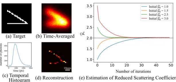
(a) Target (b) Time-Averaged

(c) Temporal

Histogram (d) Reconstruction (e) Estimation of Reduced Scattering Coefficient

10mm

Figure 2-4: Reconstruction of a 2D target within a scattering medium and the optical properties of the phantom. (a) A 2D target embedded between two phantoms. (b) When a camera observes the scattered light on the surface of the phantom, the target is blurred in space. (c) The scattered light arrives at different time points so that the measurement is blurred over time. (d) Our method successfully reconstructs the sharp edge of the target. (e) The proposed algorithm recovers the reduced scattering coefficient for various initial estimation.

and the number of iterations for each update of 𝑇 (𝑥, 𝑦) is 50. The update of 𝜇′ 𝑠 was

performed with a step size of 5 × 10−2_{. The update is terminated after 300 iterations,}

or if the change is less than 0.01%. We alternate the update of the optical properties and the target. We initialized the estimated target with the time-averaged frame and alternated the optimization over the reduced scattering coefficient 𝜇′

𝑠 and the target

𝑇 (𝑥, 𝑦) three times, starting with 𝜇′_𝑠.

Our reconstructions are the result after three updates of each parameter. As shown in Fig 2-4 (b) (c), the scattering blurs the sharp features of the target over space and time. Our reconstruction algorithm recovers the sharp edge of the target (Fig. 2-4 (d)) and recovers the optical properties of the phantom with different initialization values. The converged reduced scattering coefficient is slightly off from the ground truth be-cause of the model mismatch between Physically-accurate Monte Carlo rendering and our assumptions such as diffusion approximation and convolutional forward model.

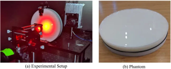
(a) Experimental Setup (b) Phantom

Figure 2-5: A picture of the experiment setup and biomimetic phantom used as a scattering media.11

2.3.2

Experiment

Implementation

Fig. 2-5 shows the physical imaging setup for the experiment. We used SuperK EX-TREME/FIANIUM supercontinuum laser from NKT photonics for the illumination source. The acousto-optic tunable filter (AOTF) was used to bandpass filter the white laser such that only light with a wavelength of around 628𝑛𝑚 was captured. The rep-etition rate of the pulsed laser is 80MHz. Photon Force 32x32 SPAD array was used to collect the ultrafast measurement. Each pixel time-stamps captured photons into 50𝑝𝑠time bin. The full width at half max (FWHM) of the total instrument response, including the pulse width of the lasers and electronic delay of the SPAD pixel, was 150𝑝𝑠.

The phantom was fabricated with epoxy resin (East Coast Resin) as a base and TiO2 powder (Pure Organic Ingredients) as a scattering agent. We followed a

pro-cedure proposed by Diep et al. [22]. The refractive index of the phantom is 1.4, which is reported in [22]. We computed the absorption coefficient and the reduced scattering coefficient of the phantom by taking measurement without any target, and fitting the parameters using the diffusion approximation model (Eq. 2.7) proposed by Patterson et al. [63]. The estimated optical properties are 𝜇𝑎 = 0.080𝑚𝑚−1 and

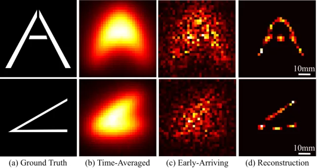
(a) Ground Truth (b) Time-Averaged (c) Early-Arriving (d) Reconstruction

10mm 10mm

Figure 2-6: Reconstruction of the targets between two biomimetic phantoms. (a) Ground truth shape of the target opening. (b) Time-averaged image of the measure-ment which is integrated over time. (c) Reconstruction from early-arriving photons. The reconstruction is noisy because the scattering media is thick and dense, and there is almost no ballistic photons. (d) Reconstruction with the proposed algorithm. 𝜇′_𝑠= 2.32𝑚𝑚−1. The two phantoms have identical optical properties, and the thick-ness of each phantom was 13𝑚𝑚, with a total of 26𝑚𝑚 scattering media.

We followed the same reconstruction steps as the simulated data. The only differ-ence is the ADMM parameters that are 𝜌 = 1, 𝜆1 = 8 × 10−4, and 𝜆2 = 10−3𝜆1. We

used higher 𝜆1 for the reconstruction on the experimental data than simulated data

to account for higher noise level.

Results

We use a black sheet of paper with a cut pattern for the target. Two opening patterns “A” and Wedge-shape were used as the targets. Without time-resolved imaging, the light exiting from the surface of the phantom is blurred, as shown in Fig. 2-6. The horizontal line of the A and the sharp edge of the wedge shape is not distinguishable from the image. While time-resolved imaging provides more information as it can capture photons exiting the phantom at different times, the reconstruction with the

early-arriving photons is noisy because the number of the ballistic photons is small. Our reconstruction algorithm successfully recovers the blurred features such as the horizontal line of “A” and the sharp edge of the wedge-shaped object, as shown in Fig. 2-5 (d). The total acquisition time to generate this result is 100 seconds for each target. The recovered reduced scattering coefficient and absorption coefficient are 2.45𝑚𝑚−1 and 0.0082𝑚𝑚−1 for “A” target, and 2.39𝑚𝑚−1 and 0.0088𝑚𝑚−1 for the wedge-shaped target.

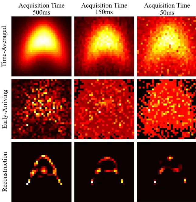
We also demonstrate the recovery of the object with a shorter acquisition time (Fig. 2-7). As expected, the reconstruction quality degrades with shorter acquisition time. We could resolve the horizontal line of “A” for acquisition times as short as 150ms. The biomimetic phantom has similar optical properties as human tissue, and the total thickness of the phantom is comparable to the thickness of our hand. Since SPAD is operating in the photon-starve regime, a stronger laser can shorten the acquisition time. This result shows the possibility for real-time medical imaging through scattering.

As discussed in Section 2.2.1, it is possible to estimate the optical properties in closed-form. However, reconstruction with closed-form estimation results in recon-struction with poorer quality than the proposed approach (Fig. 2-8). As shown in Fig. 2-9, our method robustly recovers the blur kernels of the phantom with different levels of SNR.

Finally, we also show the reconstruction with more general prior. Here, the prior term Γ(·) is the l2 norm.

Γ(v) = 𝜆 ‖𝑣‖₂. (2.23)

The minimizer of Eq. 2.20 with an l2 prior is written in a closed-form solution: ˆ

v = (P⊤P + 𝜆𝐼)−1P⊤b. (2.24)

The reconstruction results shown in Fig. 2-10 were produced using a hyper parameter 𝜆 = 0.1.

500ms

150ms

50ms

Acquisition Time

Acquisition Time

Acquisition Time

T

ime-A

veraged

Early-Ar

riving

Reconstruction

Figure 2-7: Reconstruction of the target with different acquisition times. As the acquisition time shortens, the quality of the time-averaged frame and early-arriving photon frames degrades. Our method is still able to recover the horizontal line of “A” for an acquisition time as short as 150ms.

100s Acquisition Time 500ms 500ms Acquisition Time 150ms Acquisition Time 50ms Acquisition Time

Figure 2-8: Reconstruction with previously proposed closed-form estimation of the optical properties. The closed-from estimation is susceptible to model mismatch and measurement noise as it does not target the consistency between the estimation and the measurement. x x t t t x t x x t 0 500t (ps)1000 1500 2000 Normali zed Inte nsity

(b) Acquisition Time: 100 s (c) Acquisition Time: 500 ms

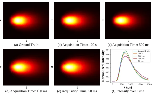
(d) Acquisition Time: 150 ms (e) Acquisition Time: 50 ms (f) Intensity over Time (a) Ground Truth

Figure 2-9: Estimated blur kernels for different acquisition time. The proposed method minimizes the different between the actual measurement and the measure-ment predicted by the forward model. Therefore, the blur kernel of the scattering medium can be estimated robustly even when the SNR is low due to short acquisition time.

10mm 10mm

Figure 2-10: Reconstruction of the 2D objects with Tikhonov regularization. The solution with l2 regularization is blurrier than the solution with l1 and total variation regularization. However, this more general assumption still recovers the feature of the objects such as the horizontal line of “A” character.

2.4

Discussion

We discuss the limitations, challenges, and potential applications of the proposed technology.

2.4.1

Practical Limitations

We demonstrated robust recovery of a 2D binary object embedded in a homogeneous volumetric scattering media with unknown optical properties. The proposed compu-tational approach extends the limitations of previous All Photons Imaging work [74]. Our technique also removes the necessity of prior measurements of the optical prop-erties of phantoms [50]. However, there are still some assumptions. For example, we assume the depth of the target is known and only consider flat surfaces for illumina-tion and detecillumina-tion. The depth can be estimated by using the automatic differentiaillumina-tion of the forward model with respect to the depth parameter, but its sensitivity is still yet to be studied. We also assumed that the scattering medium is homogeneous. However, previous works in All Photons Imaging shows that the diffusion model can be applied to layered phantoms where each layer has different optical properties [73]. Though it is out of the scope of this thesis, the proposed technique has the potential to be applied with layered, heterogeneous scattering media.

2.4.2

Trade off between efficiency, accuracy, and modeling of

complex scenes

Because our forward model is based on the diffusion approximation, the accuracy and complexity of the modeling of the scattering media are limited. While All Photons Imaging can be extended to layered media [73], the diffusion approximation does not hold for thin phantoms or spatially heterogeneous materials. To model more complex scenes accurately, the Monte Carlo Approximation [29] or combinations of the Monte Carlo approximation and the diffusion approximation [31] are better suited. However, such methods are also computationally more expensive. The proposed approach can be used as initialization to a more computationally expensive approach to achieve faster convergence.

2.4.3

Resolution Analysis

The resolution of API is limited by the invertibility of the light transport matrix P in Eq. 2.20. The light transport matrix depends on various parameters such as the temporal and spatial resolution of the ultrafast measurement, the reduced scattering coefficient, the absorption coefficient, the thickness of the scattering medium, and the spatial probing pattern of the illumination source. Therefore, the theoretical analysis of the resolution is not trivial (The first API work numerically evaluated the resolution via simulation [74]). While our work focuses on the robustness of the reconstruction without prior information of the optical properties, we illustrate the resolution performance of the proposed method experimentally. Fig. 2-11 illustrates 1D slices of the reconstruction for the mask with 2𝑚𝑚 by 10𝑚𝑚 bars with 15𝑚𝑚, 10𝑚𝑚 and 5𝑚𝑚 spacing in between. The phantoms and imaging systems that are used in this evaluation were the same as the experiments described in the results section. Similar to the results presented before, the time-averaged measurement is too blurred, and the early-arriving photons are noisy. However, our reconstruction resolves the clear peaks with 10𝑚𝑚 openings with phantoms that are 26𝑚𝑚 thick in total. While the reconstruction quality degrades, our method still manages to detect

Time-Averaged Ballistic Reconstruction Ground-Truth Time-Averaged Ballistic Reconstruction Ground-Truth 15mm Intensity (normalized) Time-Averaged Ballistic Reconstruction Ground-Truth x (mm) x (mm) x (mm) 10mm 5mm

Figure 2-11: We evaluate the practical resolution of the method using masks with two openings separated by a small spacing0.

the peaks with 5𝑚𝑚 spacing.

2.4.4

Applications

The followings are the potential applications of the proposed technology.

Medical imaging: Our transmission imaging system can be exploited to perform X-ray style imaging without using ionizing radiation, which can cause harm to the human body. Our technique is designed to use light from the visible or near-visible spectrum. Our computational framework has the potential to replace current ionizing radiation with visible light to see through scattering, making the medical imaging safer.

Fluorescent Imaging through Scattering in reflection mode: While our tech-nique can be potentially applied to the reflection-mode setting, the major challenge is the SNR. In reflection-mode imaging through deep tissue, the majority of the photons that come back to the surface do not propagate through the tissue deep enough to interact with the objects of interest. With fluorophores, such background photons can be rejected with spectral filtering as the fluorophores absorb and emit light at differ-ent wavelengths. By incorporating fluorescdiffer-ent lifetime decay in the forward model, reflection-mode imaging can be modeled with a similar model as the proposed model.

Remote Sensing through smoke, fog, and cloudy water: Our technique does not require detectors in contact with the scattering media so that it can be used for remote sensing. When smoke, fog, or cloudy water is dense and homogeneous, the proposed method can recover what is inside of such scattering media remotely.

2.5

Conclusions and Future Directions

We proposed a novel computational framework to image objects though dense vol-umetric scattering media with unknown optical properties using a simple imaging system. The use of a modern automatic differentiation framework to the physics-based forward model overcomes the challenges of previously proposed All Photons Imaging works. We experimentally demonstrated the robust recovery of 2D objects in phantoms. Our method can be used for X-ray style imaging without the use of ionizing radiation.

One of the main challenges with the proposed framework is that the imaging setup is in transmission mode. In many realistic scenarios, access to the opposing side of a scattering medium may not be available. Reflection-mode imaging is more challenging as many of the back-scattered photons that do not interact with embedded objects are also captured. One possible way to solve this problem is to use fluorescent imaging. The ‘signal’ photons can be separated from the ‘background’ by selecting a specific wavelength. This permits the use of a similar forward model as the proposed convolutional model, except that the object has exponential decay from fluorescence lifetime.

Another challenge is that the proposed framework assumes homogeneous scatter-ing media. As Satat et al. [73] demonstrated, the homogeneous assumption is still valid for reconstructing a 2D object with layer-wise heterogeneous media along the optical axis. The extension of the proposed method with a more complex forward model could address the challenges with heterogeneous scattering media in the future.

Chapter 3

Imaging tagged objects around

corners

The study of imaging around corners, also known as non-line-of-sight (NLOS) imag-ing, has advanced significantly in the past decade. While the past works in NLOS imaging mostly considered reflective targets for intensity-based measurement tech-niques, we consider tags such as fluorophores and quantum dots that absorb and emit light at different wavelengths. Previous intensity-based approaches suffer from high signal-to-background ratio as the background light has the same wavelength as the signal light that comes from the object of interest. Often, background subtraction is necessary to extract the signal light from the measurement. The low signal-to-background ratio imposes a practical challenge. A high dynamic range is required to capture small changes in the signal while the background light can saturate the sensor. Using tags, the background light can be removed by a spectral filter. The use of tags is also a natural direction for health-related imaging, where the fluorophores and quantum dots are often used to highlight regions of interest. In this chapter, we discuss the intensity-based computational imaging methods to see tagged objects around corners.

Camera

Camera Field of View

Occluder

s

o

d

n

i

l

Figure 3-1: Overview of imaging setup for imaging tagged objects around corners. A laser illuminate a spot s. The hidden tag at o absorbs and emits light at different wavelengths. A camera observes different points on the wall d1, d2, ..., d𝑚.

3.1

Forward Model

Let us consider the setting illustrated in Fig. 3-1, where a laser at i illuminates a point on a wall s, and the detector is focused at another point on the wall d. A tag (fluorophore or quantum dot) is located at o with an area 𝐴𝑜, which is sufficiently

small compared to the scale of the scene. We consider a scene consists of Lambertian surfaces with albedo 𝜌𝑠. We denote the flux of the laser projection as Φ𝑖 and the

normal of the surface as ⃗n𝑠. The radiance from the laser illumination point s towards

the tag can be written as

𝐸𝑠→𝑜 =

𝜌𝑠

𝜋Φ𝑖(︀⃗v𝑜→𝑠· ⃗n𝑠)︀. (3.1)

The total energy that a tag receives is Φ𝑠→𝑜=

∫︁

Ω𝑂

𝐸𝑠→𝑜𝑑𝜔, (3.2)

where the integral over 𝜔 is taken over the angle of vectors ⃗v𝑠→𝑜 that connects the