HAL Id: hal-01649515
https://hal.archives-ouvertes.fr/hal-01649515
Submitted on 7 Nov 2019HAL is a multi-disciplinary open access archive for the deposit and dissemination of sci-entific research documents, whether they are pub-lished or not. The documents may come from teaching and research institutions in France or abroad, or from public or private research centers.
L’archive ouverte pluridisciplinaire HAL, est destinée au dépôt et à la diffusion de documents scientifiques de niveau recherche, publiés ou non, émanant des établissements d’enseignement et de recherche français ou étrangers, des laboratoires publics ou privés.
Theoretical Study of Superposition of Macro- and
Microscale Mixing and its Influence on Mixing Kinetics
and Mixture Quality
V. Mizonov, E. Barantseva, Y. Khokhlova, Henri Berthiaux, Cendrine
Gatumel
To cite this version:
V. Mizonov, E. Barantseva, Y. Khokhlova, Henri Berthiaux, Cendrine Gatumel. Theoretical Study of Superposition of Macro- and Microscale Mixing and its Influence on Mixing Kinetics and Mix-ture Quality. Particulate Science and Technology, Taylor & Francis, 2009, 27 (4), pp.327-336. �10.1080/02726350902991015�. �hal-01649515�
Theoretical Study of Superposition of Macro- and
Microscale Mixing and its Influence on Mixing
Kinetics and Mixture Quality
V. MIZONOV
1, E. BARANTSEVA
1, Y. KHOKHLOVA
1,
H. BERTHIAUX
2, AND C. GATUMEL
21Department of Applied Mathematics, Ivanovo Power Engineering State
University, Ivanovo, Russia
2UMR CNRS 2392, Ecole des Mines d’Albi-Carmaux, Campus Jarlard,
Albi, France
The objective of this study was to build a model that describes evolution of the state of a mixture where microscale mixing (penetration of particles into the closest neighborhood of its position during a small period of time) is accompanied by macroscale mixing (periodical exchange of large parts of the mixture inside a mixing volume after a certain period of time). The mixing kinetics for segregation and nonsegregation mixtures, agitated by blades placed in a certain sequence inside the mixing volume, was modeled. The case of exchange by the halves of material was examined as well. Two variants of the exchange were examined: the parallel displacement and the symmetric turn. It is shown that there exist optimal parameters of the macroscale transitions providing the highest rate of mixing. The proposed model helps to achieve better understanding of the process and suggests some ideas to improve the design of the mixers.
Keywords blade mixing, degree of capture, granular material, macroscale mixing, Markov chain, mixing quality, transition probability
Introduction
Mixing of solids is a complex process of particle migration inside an operating volume of a mixer. To initiate the process, one has to agitate the particles strongly enough to make them overcome the threshold of coulomb friction thus bringing them to the state of interpenetration. This agitation can be realized, for example, by imposition of vibration. However, usually the rate of the process is rather small, and the equilibrium state of obtained mixtures is not homogeneous for the components, which have the tendency to segregate. In order to make the process faster and to compensate for the influence of segregation, very often a stronger kind of action is made use of, by which more-or-less large parts of material are removed from one zone of operating volume to another. Other things being equal, blades of varying geometry moving inside the operating volume can do the task.
Address correspondence to V. Mizonov, Department of Applied Mathematics, Ivanovo Power Engineering State University, Rabfakovskaya 34, Ivanovo 153003, Russia. E-mail: mizonov@home.ivanovo.ru
A mathematical model of a process helps to understand it better and can serve as a basis of calculation and design. However, the predicting ability of the model depends on the level of the process decomposition.
A common approach to model the process of mixing is the convection-dispersion model, based on the well-known Fokker–Planck equation. This approach was successfully used by Sommer (1994, 1996), especially for the case of continuous mixing. Being a partial differential equation, the Fokker–Planck equation describes the evolution of a key component concentration distribution. Also, the Fokker–Planck equation formally does not presuppose the possibility of instant or very fast transitions of the component from one zone of the operating volume to another, i.e., it fails to describe the blades’ action. Traditionally, the dispersion coefficient in this equation is used as an adjusting parameter that helps to level the calculated and the experimentally obtained concentration distribution data and automatically “averages” all the phenomena that are not taken into account by the equation itself.
An appropriate mathematical tool for modeling the process is the theory of Markov chains, which is appropriate for the process of mixing because both are related to the evolution of the state of a stochastic system. The basic idea of the Markov chain approach is to separate the operating volume of a mixer into small but finite zones (cells) and to observe the evolution of the key component concentration in the zones at discrete moments of time after a small but finite time step between them. The essence of mixing itself is migration of particles from one zone of operating volume to another. The essence of the theory of Markov chains is to describe “migration” of probabilities from one state to another in a sample space. The matrix of transition probabilities can be interpreted as a theoretical image of a mixer, acting in the sample space and transforming it. However, substantial theoretical and experimental work needs to be done in order to set up correspondence between the mixer and its matrix image.
The transition probabilities that form the matrix depend on the duration of the transition. If the duration is small enough, the transitions are allowed only to neighboring cells (states); if the duration is greater, the transitions to more distant cells can take place. Asymptotically all possible transitions are allowed, and the matrix connects directly the initial and final state of the process. Wang and Fan (1977) used the approach to describe the state of mixture after passing a static mixer. However, the approach misses the evolution of process parameters and fails to present the physical features of the mixing zone. In further works by the authors (Wang & Fan 1977; Fan et al. 1978) the model of the process, in which transitions only to the neighboring cells were allowed, was developed. A similar approach was used by Gyenis (1997) to describe segregation-free particle mixing.
The general strategy of application of the theory of Markov chains to model different processes in chemical engineering and powder technology is described by Tamir (1998) and Berthiaux et al. (2004, 2005). The attempt to describe the evolution of the homogeneity of a mixture when different conditions of mixing are realized at each transition (or at several of them) is presented below.
Description of the Model and Governing Equations
Following the general strategy of application of the theory of Markov chains, let us divide the operating volume of a mixer into m perfectly mixed cells of identical
volume placed in columns. Of course, the 1-D presentation of the volume is a very rough presentation thereof, but on the other hand it allows the demonstration of the effects of the first order of importance. The state of a key component in the mixture can be presented as the column vector S= !Sj" where j= 1# 2# $ $ $ # m is the cell
number, and Sj is the relative volume content of the key component in the jth cell related to its total volume in all the cells. Suppose that we observe the state step-by-step after the finite time intervals %t. In this case, the current time can be expressed as tk = &k − 1'%t where k = 1# 2# $ $ $ is the transition number that
can also be treated as a discrete analogue of time. The state of the mixture S changes from one transition to another. These changes can be described by the recurrent matrix equation:
Sk= PkSk−1 (1)
where Pk is the matrix of transition probabilities that can vary from one transition
to another.
In a general case the matrix of transition probabilities is a square m× m matrix. The jth column of it is associated with the jth cell of the chain. The probability Pij in the ith row of the column is related to the transition from the jth to the ith cell. The term “probability” is related to a single particle of the key component in the cell. It can also be interpreted as the relative volume of the key component transiting from the jth to the ith cell during %t (related to the total current volume of the key component in the cell).
Let us call such transition, at which particles are allowed to transit from the given cell only to the neighboring cells, the microscale transition. These transitions occur due to material agitation and are directly connected with the Fokker–Planck equation. For a general case, downward and upward transition probabilities are not equal to each other due to segregation in one or the other direction. Let us suppose that Pj+1#j > Pj−1#j, having in mind that the numbering of the cells begins
from above. In this case segregation occurs in the downward direction. These transitions can be separated to the symmetrical part characterized by the probability d and nonsymmetrical part characterized by the probability v. Thus, we get the following presentation for the transition probabilities: Pj−1#j = d, Pj+1#j = d + v. In this case the matrix of transition probabilities, which is associated with the dispersion equation and written for five cells, can be written as:
PD= ⎡ ⎢ ⎢ ⎢ ⎢ ⎢ ⎣ 1− d − v d 0 0 0 d+ v 1− 2d − v d 0 0 0 d+ v 1− 2d − v d 0 0 0 d+ v 1− 2d − v d 0 0 0 d+ v 1− d − v ⎤ ⎥ ⎥ ⎥ ⎥ ⎥ ⎦ (2)
where d= D%t/%x2# v= V%t/%x# D is the dispersion coefficient, V is the average
velocity of particle downward segregation, and %x is the length of cells. This matrix acts on the state vector at each transition. The transition probabilities depend on the time step %t and on the spatial step %x, which must be chosen with such values that no negative elements in the matrix Equation (2) appear, i.e., 1− 2d − v ≥ 0. Physically it means that the amount of the key component that is removed from a cell in the both directions during a transition cannot be larger than the amount the cell contained before the transition. It is necessary to emphasize that in this study
we deal with linear models where the transition probabilities do not depend on the key component concentration in a cell, i.e., with the case of the state-independent matrix.
Let us also introduce the matrix of macroscale transitions PB, which allows
transitions to cells more distant than the neighboring ones. For example, it can imitate the action of blades in a blade mixer, or other variants of macroscale events. As in Equation (1), its main diagonal contains the probabilities to stay within corresponding cells during one transition, but probabilities to transit should be placed in those rows to which the particles transit. Some examples of the matrix PB
will be shown below.
Suppose that the matrix PD (i.e., the microscale mixing) acts during L transitions, and then the matrix PB (i.e., macroscale mixing) acts during one
transition. Thus, the cycle of mixing consists of L+ 1 transitions, and the evolution of the state vector within the cycle can be described by the following recurrent equation:
Sk+i = P
DSk+i−1# i = 1# 2# $ $ $ # L# and Sk+L+1 = PBSk+L (3)
where i is the number of the current microscale transition. It is necessary to emphasize that the matrix can also vary from one macroscale transition to another. Thus, the above-formulated model allowed the description of mixing kinetics when the microscale mixing alternates with the macroscale mixing.
Numerical Experiments
Macroscale Transitions Caused by Material Displacement from One Cell Only (Imitation of Small Blade Action)
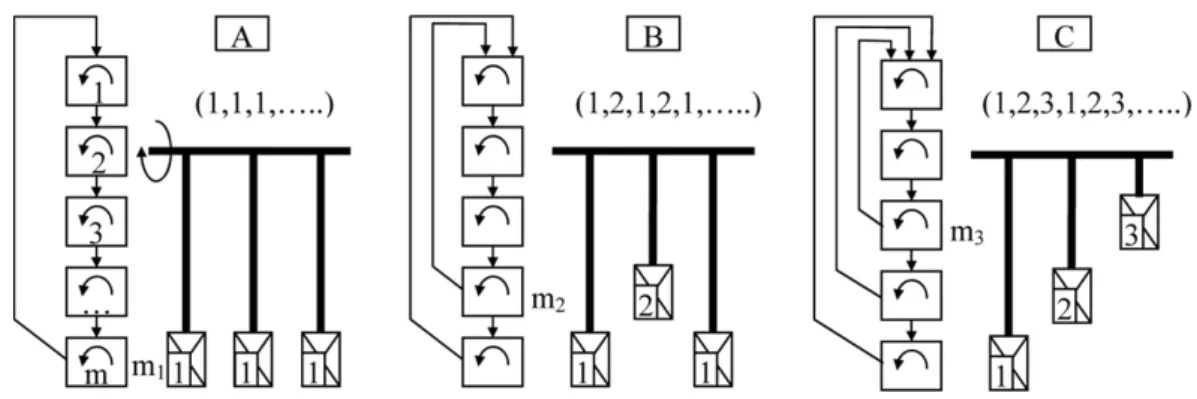
Let us examine the process schematically presented in Figure 1. The operating volume is presented as five perfectly mixed cells. The microscale mixing can occur at each transition. Figure 1 shows several variants of the macroscale transitions that imitate action of blades interacting with a cell when the blade sends the part ( of the key component from the cell to the top, i.e., to cell 1. However, formally it is better to speak about macroscale mixing due to convective fluxes where the cycle should be closed via fluxes through the series of neighboring cells. For example, for case A the cycle is 5→ 1 → 2 → 3 → 4 → 5 where the transition from cell 1 to
Figure 1. Various cycles of blade interaction with material: case A, all blades interact with the same cell at the bottom; case B, alternation of two blades interacting with two different cells; case C, alternation of three blades interacting with three different cells.
cell 5 occurs directly (without any interaction with the other cells). If we deal with a real blade, it elevates the material through other layers above and interacts with them. Nevertheless, if the size of the blade is small enough, this distortion can be approximately neglected.
The blades are placed in a certain order, which defines the sequence of their actions also shown in the figure. The arrangement of the blades on the shaft is shown conditionally. It can correspond to a continuous blade mixer with homogeneous perfect plug flow in the axial direction, but the blades can be placed in one plane that corresponds to batch mixing.
The matrix of macroscale transitions written, for instance, for case B (blade 2), has the following form:
PB= ⎡ ⎢ ⎢ ⎢ ⎢ ⎢ ⎣ 1− ( 0 0 ( 0 ( 1− ( 0 0 0 0 ( 1− ( 0 0 0 0 ( 1− ( 0 0 0 0 0 1 ⎤ ⎥ ⎥ ⎥ ⎥ ⎥ ⎦ (4)
where part ( of the key component is sent to the top from cell 4. It is obvious that ( should be less than 1. In all numerical examples presented below L= 1. The homogeneity of mixture is estimated by the standard deviation:
)= ' ( ( )1 m m * j=1 + Sj − 1 m ,2 (5) Figure 2 illustrates the influence of parameter ( on the nonsegregation mixture homogeneity after 10 transitions (left) and mixing kinetics (right) for various structures of macroscale transitions. It is obvious that ) has the minimum with respect to ( lying in the range (= 0$5# $ $ $ # 0$6, and the best mixture quality is provided by blade arrangement C.
Figure 2. Influence of parameter ( on the mixture homogeneity after 10 transitions (left) and mixing kinetics (right) for various structures of macroscale transitions: × for case A, + for case B, ∗ for case C.
Figure 3. Influence of the structure of macroscale transitions on the mixing kinetics in the case of downward segregation: − for pure micro, × for case A, + for case B, ∗ for case C.
The situation changes when the key component has the tendency to segregation. The data shown in Figure 3 for v= 0$1 demonstrate that the best mixture quality is provided by blade arrangement A. However, the rate of mixing is much faster and the mixture quality is much better at any structure of the macroscale transitions than in the case of their absence.
Macroscale Transitions Caused by Exchange of the Halves of Material Volume Now let us examine some of the cases when the large zones of operating volume can exchange their positions. This can be achieved with large blades the size of which is commensurable with the size of the operating volume, by periodical revolving of the operating volume and other methods. These exchanges can be also called macroscale transitions that involve several cells at once.
Two variants of these macroscale transitions are shown in Figure 4. One of them is the parallel displacement of the halves without their turning around the central axis; the other is the symmetric turn around this axis. It is necessary to emphasize that the chains modeling the process are not bound to the mixer body, and the numbering of the cells remains the same after a macroscale transition. If there is no segregation, the latter case gives nothing for the mixing kinetics except
Figure 4. Two variants of macroscale transitions: 1, parallel displacement; 2, symmetric turn ((= 1).
additional delay for each macroscale transition in the model. This, however, is not the case if segregation occurs.
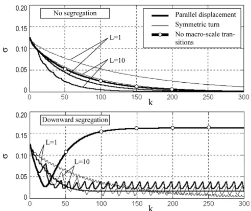
The example of macroscale transition matrices for the four-cells chain is shown below: PB= ⎡ ⎢ ⎢ ⎢ ⎢ ⎢ ⎢ ⎢ ⎢ ⎢ ⎢ ⎢ ⎢ ⎣ 1− ( 0 0 0 ( 0 0 0 0 1− ( 0 0 0 ( 0 0 0 0 1− ( 0 0 0 ( 0 0 0 0 1− ( 0 0 0 ( ( 0 0 0 1− ( 0 0 0 0 ( 0 0 0 1− ( 0 0 0 0 ( 0 0 0 1− ( 0 0 0 0 ( 0 0 0 1− ( ⎤ ⎥ ⎥ ⎥ ⎥ ⎥ ⎥ ⎥ ⎥ ⎥ ⎥ ⎥ ⎥ ⎦ for Case 1 (6) and PB= ⎡ ⎢ ⎢ ⎢ ⎢ ⎢ ⎢ ⎢ ⎢ ⎢ ⎢ ⎢ ⎢ ⎣ 1− ( 0 0 0 0 0 0 ( 0 1− ( 0 0 0 0 ( 0 0 0 1− ( 0 0 ( 0 0 0 0 0 1− ( ( 0 0 0 0 0 0 ( 1− ( 0 0 0 0 0 ( 0 0 1− ( 0 0 0 ( 0 0 0 0 1− ( 0 ( 0 0 0 0 0 0 1− ( ⎤ ⎥ ⎥ ⎥ ⎥ ⎥ ⎥ ⎥ ⎥ ⎥ ⎥ ⎥ ⎥ ⎦ for Case 2 (7) Figure 5 illustrates evolution of the state vector and influence of the interval L between successive macroscale transitions on the mixture quality after 80 transitions for Case 1 without segregation.
It can be seen that the mixture quality has the flat maximum with respect to L lying in the range 5# $ $ $ # 10.
Figure 5. Evolution of the key component content for d = 0$2 and L = 10 (left) and influence of the period of macroscale transitions on the mixture homogeneity after 80 transitions (right): symbol × is for d = 0$05, + for d = 0$1, ∗ for d = 0$2, and horizontal solid lines for no macroscale transitions.
Figure 6. Influence of macroscale transitions parameters and their structure on mixing kinetics for different components.
Figure 6 shows influence of some of macroscale transition parameters and their structure on mixing kinetics. The upper graph is related to the case of no segregation. The parallel displacement strongly improves the mixing kinetics in comparison to pure microscale mixing, and L= 10 provides much better results than L= 1. The symmetric turns give no gain in this case. The situation changes practically to the opposite if segregation occurs (the lower graph). The maximum mixture quality for pure microscale mixing comes first, but the quality itself is not too good, and it gets worse rapidly after the optimum point. The frequent macroscale transitions provide lower rate of mixing but better quality of the mixture that is reached later on. The lowest rate of mixing but the highest quality of the mixture can be reached using the frequent (L= 1) symmetric turns, at which the mixture quality slightly oscillates with time around the lowest value of ). This result validates the efficiency of static revolving mixers for the materials inclined to segregate. The case L= 10 gives much stronger asymptotic oscillation of the standard deviation ), which is not good from the viewpoint of mixture quality.
Investigation of the influence of ( on ) shows that an optimum exists here too. The optimum value of ( is close to 0.5 for no segregation and becomes larger with more extensive segregation.
The model described here can be generalized to the case of continuous blade mixing. If the objective of the study is mixing in the longwise direction only, the Fokker–Planck equation, or a one-dimensional chain corresponding to it, can be used. However, in this case the model cannot describe the crosswise mixing and possible segregation in this direction, which has a great influence on mixture quality at output. At least a two-dimensional model, in which the columns of cells are placed one after another, must be used. Additional transitions between columns appear in such a model, and the dimension of the model increases strongly.
In particular, the blade crossing a mixture at the bottom of the holdup in a column sends a part of material to the top of the column and a part to the bottom cell of the next column. The same strategy of modeling as described above can be used to build the two-dimensional model. However, its detailed description is beyond the objectives of the present article.
Conclusions
A cell model of combined micro- and macroscale mixing where the macroscale mixing can imitate blade action is proposed. It is shown that the efficiency of this action depends on properties of materials to be mixed (in particular, on their tendency to segregation), on the position of the blades inside a mixing volume, and on the part of the material that can be transported by the blade to the top of the mixture during one transition. The rational distribution of blades over the mixing volume is found and the optimum value of the transported part of the material is defined. A model with exchange of large parts of material in the volume is proposed as well, and two variants of the exchange are examined: parallel displacement and symmetrical turn. It is shown that the parallel displacement is more effective for nonsegregating components while the symmetric turn is more effective for segregating components. The results can play an important role in the synthesis of mixing systems and mixer design.
Nomenclature
D dispersion coefficient, m2/s
d dimensionless dispersion coefficient, dispersion transition probability i number of cell material transits to and from the jth cell
j current cell number k transition number
L number of microscale transitions between the macroscale one m number of cells in a chain
Pij probability of transition from the jth to the ith cell during %t
PB matrix of transition probabilities for macroscale mixing PD matrix of transition probabilities for microscale mixing S state column vector
t time, s V velocity, m/s
v dimensionless convection coefficient, convection transition probability Greek letters
( part of material captured and transported by blade ) standard deviation
References
Berthiaux, H. & V. Mizonov. 2004. Applications of Markov chains in particulate process engineering: A review. Can. J. Chem. Eng. 85 (6): 1143–1168.
Berthiaux, H., K. Marikh, V. Mizonov, D. Ponomarev, & E. Barantzeva. 2004. Modelling continuous powder mixing by means of the theory of Markov chains. Part. Sci. Technol. 22 (4): 379–389.
Berthiaux, H., V. Mizonov, & V. Zhukov. 2005. Application of the theory of Markov chains to model different processes in particle technology. Powder Technol. 157: 128–137. Fan, L. T., F. S. Lai, Y. Akao, K. Shinoda, & E. Yoshizawa. 1978. Numerical and
experimental simulation studies on the mixing of particulate solids and the synthesis of a mixing system: Mixing process and stochastic motion of mutually noninteracting particles. Comput. Chem. Eng. 2 (1): 19–32.
Gyenis, J. 1997. Segregation-free particle mixing. In Proceedings of the 2nd Israel Conference for Conveying and Handling of Particulate Solids. Jerusalem, pp. 11.1–11.10.
Sommer, K. 1994. Continuous powder mixing. In Proceedings of the 1st International Particle Technology Forum, Denver, 1994. Part III, pp. 343–349.
Sommer, K. 1996. Mixing of particulate solids. KONA 14: 73–78.
Tamir, A. 1998. Applications of Markov Chains in Chemical Engineering. Amsterdam: Elsevier. Wang, R. H. & L. T. Fan. 1976. Axial mixing of grains in a motionless Sulzer (Koch) mixer.
Ind. Eng. Chem. Process Des. Dev.15 (3): 381–388.
Wang, R. H. & L. T. Fan. 1977. Stochastic modeling of segregation in a motionless mixer. Chem. Eng. Sci.32: 695–701.