Excitation of wood joist floors with the standard rubber ball

Publisher’s version / Version de l'éditeur:

Vous avez des questions? Nous pouvons vous aider. Pour communiquer directement avec un auteur, consultez la première page de la revue dans laquelle son article a été publié afin de trouver ses coordonnées. Si vous n’arrivez pas à les repérer, communiquez avec nous à PublicationsArchive-ArchivesPublications@nrc-cnrc.gc.ca.

Questions? Contact the NRC Publications Archive team at

PublicationsArchive-ArchivesPublications@nrc-cnrc.gc.ca. If you wish to email the authors directly, please see the first page of the publication for their contact information.

https://publications-cnrc.canada.ca/fra/droits

L’accès à ce site Web et l’utilisation de son contenu sont assujettis aux conditions présentées dans le site LISEZ CES CONDITIONS ATTENTIVEMENT AVANT D’UTILISER CE SITE WEB.

Inter-Noise 2009 [Proceedings], pp. 1-9, 2009-08-23

READ THESE TERMS AND CONDITIONS CAREFULLY BEFORE USING THIS WEBSITE. https://nrc-publications.canada.ca/eng/copyright

NRC Publications Archive Record / Notice des Archives des publications du CNRC :

https://nrc-publications.canada.ca/eng/view/object/?id=62a8d8e3-9df0-4067-b0b4-578666181470 https://publications-cnrc.canada.ca/fra/voir/objet/?id=62a8d8e3-9df0-4067-b0b4-578666181470

NRC Publications Archive

Archives des publications du CNRC

This publication could be one of several versions: author’s original, accepted manuscript or the publisher’s version. / La version de cette publication peut être l’une des suivantes : la version prépublication de l’auteur, la version acceptée du manuscrit ou la version de l’éditeur.

Access and use of this website and the material on it are subject to the Terms and Conditions set forth at Excitation of wood joist floors with the standard rubber ball

http://irc.nrc-cnrc.gc.ca

Exc it at ion of w ood joist floors w it h t he st a nda rd

rubbe r ba ll

N R C C - 5 1 3 1 0

S c h o e n w a l d , S . ; Z e i t l e r , B . ; N i g h t i n g a l e , T . R . T .

A u g u s t 2 3 , 2 0 0 9

A version of this document is published in / Une version de ce document se trouve dans: InterNoise 2009, Ottawa, Ontario, Aug. 23-26, 2009, pp. 1-9.

The material in this document is covered by the provisions of the Copyright Act, by Canadian laws, policies, regulations and international agreements. Such provisions serve to identify the information source and, in specific instances, to prohibit reproduction of materials without written permission. For more information visit http://laws.justice.gc.ca/en/showtdm/cs/C-42

Les renseignements dans ce document sont protégés par la Loi sur le droit d'auteur, par les lois, les politiques et les règlements du Canada et des accords internationaux. Ces dispositions permettent d'identifier la source de l'information et, dans certains cas, d'interdire la copie de documents sans permission écrite. Pour obtenir de plus amples renseignements : http://lois.justice.gc.ca/fr/showtdm/cs/C-42

Excitation of wood joist floors with the standard rubber ball

Stefan Schoenwalda Berndt Zeitlerb Trevor Nightingalec

Institute of Research in Construction National Research Council Canada Ottawa ON K1A 0R6 Canada

ABSTRACT

Characterizing and rating the impact sound isolation of floors and of building structures are important issues in building acoustics. During impact tests the floor is excited structurally with standard impact sources that exert forces normal to the floor like e.g. as occurs when a person is walking. However, different kinds of impact sources exist and unfortunately the excitation spectrum of the lightweight tapping machine according to ISO 140-7 differs significantly from the heavy sources according to JIS A 1418-2 (the rubber ball and the tire that are dropped from a defined height on the floor). Excitation due to a drop of a rubber ball is considered in the course of a current research project on the impact sound isolation of lightweight wood joist floors. In this paper the change of the impact sound level with drop height of the ball is investigated. In a first step the change of the impact force caused by the ball is predicted with an analytical model and the results are compared to experiment.

a

Email address: stefan.schoenwald@nrc-cnrc.gc.ca b

Email address: berndt.zeitler@nrc-cnrc.gc.ca c

Email address: trevor.nightingale@nrc-cnrc.gc.ca

1. INTRODUCTION

Rating the impact sound isolation of floors in the laboratory or buildings is one important issue in building acoustics and usually impact tests are carried out to characterize floors. Currently testing is done according to different international and national standards. Basically all standards follow the same test procedure - the floor is excited structurally by a standardized impact source in one room and the sound pressure level due to the impact is measured in a second receiving room. Besides differences in the measurement of the receiving sound power and the post processing, e.g. averaging, weighting and normalization, the most obvious difference between

the standards is the used impact source. In ISO 140-7 a tapping machine is defined that is probably the most commonly used impact source worldwide. Five steel hammers of 0.5 kg weight are lifted by a shaft that is driven by an electrical engine and dropped with a frequency of 10 Hz from a height of 4 cm. Unfortunately, the impact force spectrum that is applied by this light impact source to lightweight framed floors does not correlate well with a real human walker or a child jumping. Therefore other impact sources - a modified tapping machine with rubber pads between the hammers and the floor and a so-called heavy/soft impact source - are presented in the Annexes of ISO 140-11.

The latter one, a rubber ball, is dropped from a 1 m height and will be the focus of this paper. It was developed in Japan and originally defined in JIS A 1418-2 along with a second heavy impact source – the tire or so-called “bang machine”. The tire is a small car wheel that is lifted mechanically and dropped from a height of 85 cm. Even though the ball impact source was developed more recently it soon became more popular than the tire because the ease of its handling. Often still the tire is preferred because of the higher impact sound pressure levels that are beneficial if it is applied in a noisy environment, like on a construction site, or for the measurement of flanking transmission.

A simple solution to obtain better signal-to-noise ratio for the ball impact might be to increase the sound pressure level in the receiving room by raising the drop height of the ball and normalizing the results afterwards to the standard drop height of 1 m. However, this solution is only feasible if the force as well as the response of the floor due to ball impact is linear with the drop height. Hence as a first step the blocked ball force is predicted with a simple model for different drop heights and results are compared to experiment to determine the characteristics and limits of the ball source.

2. PREDICTION OF THE BLOCKED BALL FORCE

In this paper a rather simple prediction model of Hubbard et al.1 is applied to predict the force due to the impact of the JIS ball from different drop heights. Besides the geometry and the mass of the ball that are well defined in JIS A 1418-2 only the E-modulus and Poisson’s ratio of the ball material have to be known for the prediction model.

The geometry of a hollow elastic spherical shell - like balls - can be simply described by the so-called thinness ratio R/h which is the ratio of the radius, R, and the wall thickness, h, as shown in Figure 1. The thinness ratio of the ball impact source is approximately 3 and is rather small compared to a table tennis ball (R/h = 47) for which the applied model originally was developed. However, Hubbard pointed out that for tennis balls with a thinness ratio of around 5 which is close to the one of the impact ball his prediction model is expected to deliver even better results than for table tennis balls.

B. Deformation of a Hollow Elastic Spherical Shell

In the applied prediction model two regimes of compression are considered, namely small and moderately large shell deflections δ.

At the beginning of the impact - just before contact of the shell and the surface – the shell is assumed to move with uniform impact velocity in z-direction normal to the rigid surface. Directly after contact, in the first regime, part of the shell that is in contact with the rigid structure flattens and remains in contact with the surface. This flattened cap of the shell has no velocity (it is at rest) for small deflections whereas the remainder of the shell moves uniformly with a reduced centre of mass velocity ₀, as shown on the left in Figure 1.

The second regime occurs if the impact velocity is sufficiently high and the critical deflection δc is exceeded. The shell buckles to minimize its strain energy of deformation, i.e. the

central area of the flattened shell snaps through in the hollow interior as shown on the right in Figure 1. At the point of maximal shell deflection all dynamic energy of the shell is transformed into elastic energy due to shell compression and the whole shell is at rest (it has no velocity).

The whole process is reversed during the restitution phase. The shell starts to move in the opposite direction and elastic energy is transformed back into dynamic energy.

Figure 1: Deflection of a hollow spherical shell at impact on a rigid surface – a) small and b) moderate large shell deflection

The critical deflection δc depends on the shell thickness and the internal pressure and was found

to occur for unpressurised table tennis balls at δc/h = 2.0…2.2.2,3 For the ball impact source the

ratio of the maximum deflection investigated in this paper is much smaller δmax/h  1 and thus

only the first regime for small deflections is considered in this paper. C. Ball Forces

In the prediction model two force components are considered and the total contact force FT that

is exerted by the ball during normal impact on a flat rigid surface is the sum of both the force FB

due to the shell stiffness and force due to the increase of internal pressure FG.

Most important is the force FB due to elastic deformation of the shell during impact. For

small deflections Reissner4 developed equations for a small indentation of a segment of an elastic spherical shell by a point force at the crown. The force FB due to the shell stiffness is given by

Equation 1 and is a function of the deflection δ, the radius R, the usual plate bending stiffness B and the reduced wall thickness hr. Latter ones are given in equations 2 and 3 and are additionally

a function of the wall thickness h, the modulus of elasticity E, and the Poisson’s ratio ν.  r B h R B F  8 . (1)













The other contact force FG is associated with the gas pressure inside the shell. This component is

of secondary order for the ball impact source. The initial internal pressure p0 of the ball impact

source is assumed to be equal to the external atmospheric pressure pa. The impact ball has a

small hole in its shell to ensure that the force component FG is independent of external pressure

changes e.g. due to geographical conditions or weather. However, during impact the ball is flattening against the surface and the internal volume decreases. Thus the internal gas pressure increases in proportion to ball deflection since the radius of the shell is assumed not to expand and airflow through the small hole in the shell cannot equalize the increase of internal pressure

during the short contact time. The force FG is much smaller than the force associated with the

stiffness of the shell and possibly negligible for small ball deflections. It is taken into account for the ball impact source for completeness and for small ball deflections it is given by equation 4 where the ratio of specific heats for air is γ = 1.4.

                                                     R R R p p R p F a g a G 1 2 2 3 1 1 2 . with p0  pa  pg (4)

D. Equation of Motion for Ball Impact

The dynamic energy of the shell is proportional to the centre of mass velocity  which is the time derivative of its deflection δ since for small deflections it is assumed that the whole shell with exception of its flattened cap moves uniformly. On the other hand its elastic energy is proportional to the components of elastic force presented in the previous section. Both dynamic and elastic energy can be related since there has to be a conservation of momentum during impact.

The momentum of the shell is the product of the centre of mass velocity  and its dynamic mass both of which change during impact as outlined above in section 2B. The mass Mc of the

flattened cap is at rest and reduces the dynamic mass of the shell which is given by Equation 5. It is a function of the total mass of the shell M and of course also a function of shell deflection.

 R M M_c 2  . (5)

When the momentum relationship is applied the equation of motion of the ball is given by equation 6 for normal impact on a rigid flat surface

 





 

 

 

where the second term on the left side represents a dissipative momentum flux term that occurs only during restitution5 and hence the Heaviside function H is defined as follows:

 

H . for 0 (7)

 

H . for 0 (8)

E. Solving the Equation of Motion and Data Processing

Equation 6 can be solved numerically for a given time span with a commercial software package as an initial value problem after the substitution method is applied to transform the differential equation of second order into set of two coupled differential equations of first order.

The time span starts at time t0 = 0 just before impact and two initial conditions have to be

known at this time point. First the most obvious initial condition is the shell deflection δ0 = 0.

Second also the initial impact velocity 0 of the ball impact source is known at the start time. It

depends on the constant of gravitation g and drop height hD of the ball.

D h g 2 0   _{. (9)}

The time span for evaluation of the set of differential equations is chosen to be 1 s which is the time span for averaging the impact force exposure level LFE according to Annex 1 of JIS A

1418-2:2000. The number of time samples in this time span was 44100 which equals the sampling rate of the measurement system that was used to record the time history of force in experiment.

For the considered drop height and for all time samples the numerical solver for the set of differential equations returns the shell deflection δ. In a second step the time history of the impact force is calculated using equation 1 and equation 4.

In the last stage of data processing a FFT is performed on the time history of the predicted impact force and the RMS-values are band filtered in the frequency domain to obtain the octave band spectrum of the impact force exposure level LFE according to JIS A 1418-2:2000.

3. MEASUREMENT SETUP

The predicted results are compared to measured results to validate and gauge the accuracy of the applied prediction model and to gather more information of characteristics of the ball impact source.

An impact ball (Type YI-01, Rion) was dropped on a force plate (Impulse-Force-Transducer PF-10, Rion) located on a rigid concrete floor. The time history of the blocked ball force was measured with a A/D-data acquisition card connect to a standard desktop computer. The sampling rate of the measurement system was 44.1 kHz and a time span of 1 s that contains the impulse due to the ball drop was used for the further data processing. Data processing to obtain the impact force exposure level LFE was done identically to the predicted forces outlined

in section 2E.

To investigate the change of the impact force five ball drops were carried out at each heights, hD, ranging from a minimum height of 10 cm to a maximum height of 160 cm in 10 cm

steps. An adjustable microphone stand was used to ensure the correct drop height. The measured forces were averaged in the frequency domain. The standard deviation of the forces of the five ball drops was surprisingly small for all heights.

4. COMPARISION OF PREDICTION AND EXPERIMENT

For the prediction of the impact forces the geometrical and material properties of the Rion ball impact source have to be known as input data. The geometry (R = 89 mm, h = 32 mm) and the total mass (M = 2.5 kg) of the ball is well-defined in JIS A 1418-2:2000, whereas the elastic properties of the material are defined indirectly by the composition of the silicone rubber. Hence literature values are used in the prediction model for the modulus of elasticity (E = 1.65 N/mm2) and the Poisson’s ratio (ν = 0.49).

A. Time History, Maximal Ball Force and Impact Time

First the raw measurement and prediction data is compared for the different drop heights. Two constants that roughly describe the time history of the force are the impact time and the maximum impact force.

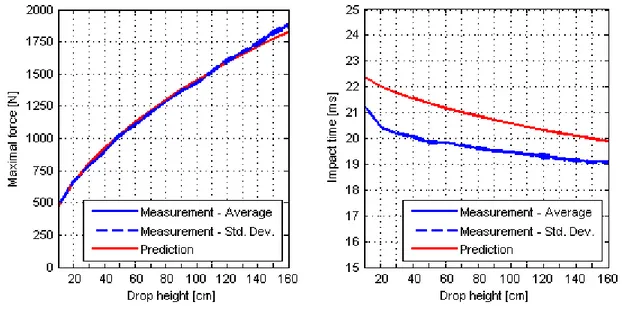
The maximal force is presented on the left in Figure 2 for drop heights 10 cm to 160 cm in 10 cm steps. The blue solid graph is the average of the five measured ball drops for each height and the blue dashed lines indicate the standard deviation that is very small and almost not visible in the figure. The maximal impact force is 465 N for a 10 cm drop height. The force increases as the impact speed in Equation 9 by a factor 2 per doubling of height. The red line shows the predicted maximal force also follows this trend and agrees very well with the measurement results. At 160 cm drop height both the predicted and measured force are about 1800 N.

The impact time is the duration of the contact between the ball and the rigid surface or force plate and is shown on the right in Figure 2 for all drop heights. The blue lines are again the measured results. Again the standard deviation of the five drops is very small, i.e. less than 0.1 ms. The measured average impact time is about 21 ms for 10 cm and 19 ms for 160 cm drop

height. The prediction (red line) overestimates the impact time by about 1 ms for all drop heights. However, at the standard drop height of 100 cm both the prediction (20.5 ms) and measurement (19.5 ms) fulfill the requirements (20 ms ± 2 ms) according to JIS A 1418-2:2000.

Figure 2: Maximal force (left) and impact time (right) as function of the drop height of the impact ball - Comparison between prediction and measurement

At first glance the difference between predicted and measured impact time seems to be rather large. In Figure 3 both are related to the magnitude of the measured values. The prediction model either overestimates or underestimates the maximal impact force by only less than 3% for all drop heights. For the impact time the error is slightly larger and about 6% in average for all drop heights which is still very small.

Figure 3: Relative error of predicted maximal impact force and impact time as function of drop height The predicted and measured time histories of the force are compared in Figure 4 for all considered drop heights. The predictions on the right seem to be almost symmetric around their maximum and the slope seems to be equal during compression and restitution. Thus the dissipative momentum flux term (in Equation 6 which is only valid for the restitution phase) is small and causes only a slight distortion of the graphs.

The measured time histories on the left are the mean of the five ball drops for every drop height. Averaging is done in the frequency domain and afterwards an inverse FFT is carried to obtain an “average” time history. The shape of the measured curves is very different from the predicted. The increasing slope during compression phase is much bigger for the measurement

than for the prediction whereas during the restitution phase both measured and predicted graphs are quite similar. Further the measured time histories show an oscillating behavior with a period that is a small fraction of the impact time. Both the steeper initial slope and the oscillations are possibly related to resonances of the ball and the first radial mode of the contact plate of the impulse-force-transducer that are not taken into account in the prediction model.

Figure 4: Time history of impact force for drop heights from 10 cm to 160 cm – Measurement (left) and prediction (right)

B. Impact Force Exposure Level LFE

In JIS A 1418-2:2000 the heavy impact sources are further characterized by the spectrum of the impulse force exposure level LFE. Limits are given for the allowable force levels in octave bands

from 31.5 Hz to 500 Hz. Thus the measured and predicted forces are processed as described in section 2E to obtain LFE.

On the left in Figure 5 LFE is shown for a limited number of drop heights (due to legibility

aspects). Measured data is only presented below 1000 Hz because of the limit in the frequency range of the force plate. Blue lines are measured and red are predicted LFE. The thick lines are

the drop height of 100 cm and the measured LFE for this height within the limits of JIS A

1418-2:2000 indicated by the black lines. The prediction for 100 cm agrees very well to measurement at 31.5 Hz and 63 Hz and decreases almost linearly with 9 dB per octave band besides a small offset between 63 Hz and 125 Hz. The measured LFE decreases less and not linearly with

frequency. Thus the prediction model grossly underestimates LFE above 125 Hz.

Further data is presented for 10 cm, 20 cm, 40 cm, 80 cm and 160 cm which is always a doubling of height and additionally for drop height of 120 cm. The predicted LFE show all the

same trend for these heights but are shifted in all octave bands by a constant value that depends on drop height. The measured forces roughly follow all the same trend but the shift between the graphs is frequency dependent.

To further investigate the frequency dependency, differences of LFE for all drop heights and

for 100 cm are presented on the right in Figure 5. For the predicted data the differences are almost equal in all octave bands whereas the measured show a distinct frequency dependency with increasing differences at higher frequencies. Further Figure 5 shows that the error in LFE

due to a small uncertainty in the standard drop height is quite small since the measured level difference for drop height 100 cm ±20 cm is less than ±3dB.

Increase of drop height

Increase of drop height

Figure 5: Measured and predicted impact force exposure level LFE for drop heights from 10 cm to 160 cm – Octave band spectrum (left) and normalized to 100 cm drop height (right)

In Figure 6 the increase of LFE is plotted as function of ratio of the drop height for the full set of

data. The increase is linear for all octave bands but of course the slope of the lines varies strongly for the measured data on the left. On the right the predicted LFE increases with 3 dB per

doubling of drop height in all octave bands except at 63 Hz, where the increase is slightly bigger.

Figure 6: Increase of impact force exposure level LFE with drop height– Measurement (left) and prediction (right)

Since Figure 6 clearly indicates that LFE increases linearly with drop height a linear curve fitting

is done. The slope of the lines in Figure 6 is determined for all octave bands and shown in Figure 7 as increase of LFE per doubling of drop height for all octave bands. Again the

agreement between prediction and measurement only matches for 31.5 Hz and 63 Hz since the predicted values are about 3 dB higher in all octave bands. The little peak at 63 Hz is caused by the change of the frequency content of the impulse, i.e. by the shift of the so-called first contact resonance, due to the decrease of impact time with drop height. The measured data increases

with frequency and the change of LFE per doubling of drop height even reaches 16 dB at

1000 Hz. Thus the impact ball cannot be considered to be a linear source.

Figure 7: Increase of impact force exposure level LFE per doubling of drop height

4. CONCLUSIONS

In this paper a rather simple prediction model of the impact of a hollow spherical shell on a rigid surface is applied for the prediction of the impact force exposure level LFE of the ball impact

source for different drop heights. Measurements are carried out to validate the prediction model. Good agreement was found for the maximal impact force and the impact time in the time domain. However these two quantities do not sufficiently characterize the source because only in the 31.5 Hz and 63 Hz octave bands the measurement and prediction agree well and the predicted LFE was within the limits of the JIS A 1418-2:2000. However, these octave bands

usually govern the single number rating of the impact sound isolation of lightweight floors that are considered in the future in this research project. Further for the prediction model the increase of LFE with drop height is linear excluding the 63 Hz octave band. The measured LFE increases

differently in each single octave band with drop height making it frequency dependent, where the slope is for example at 1000 Hz 20 times bigger than at 31.5 Hz. Hence the ball is not a linear impact source. The increase is probably caused by deformations of the ball that are not taken into account in the prediction model, like e.g. the different vibration modes of the rubber shell.

Nevertheless the ball is a good alternative to other heavy impact sources or the tapping machines due to its simplicity and it is shown in this paper that the error due to small changes of the standard drop height is rather small.

ACKNOWLEDGMENTS

We gratefully acknowledge the help of Christoph Höller of the RWTH Aachen, Germany who did all the measurements that are presented in this paper.

REFERENCES

1

M. Hubbard and W. J. Stronge, “Bounce of hollow balls on flat surfaces”, Sports Engineering 4, 49-61 (2001) 2

D. P. Updike and A. Kalnins, “Axisymmetric post-buckling and nonsymmetric buckling of a spherical shell compressed between rigid plates”, ASME Journal of Applied Mechanics 94, 172-178 (1972)

3

R. Kitching, R., Houlston and W. Johnson, “Theoretical and experimental study of hemispherical shells subjected to axial loads between flat plates”, International Journal of Mechanical Sciences, 17, 693-703 (1975)

4

E. Reissner, “On the theory of thin, elastic shells”, Contributions to Applied Mechanics, H. Reissner Anniversary

Volume, J.W. Edwards, Ann Arbor, MI, USA, 231-247 (1949)

5

A. L. Percival, “The impact and the rebound of a football”, The Manchester Association of Engineers, Session 1976-77, 5, 17-28 (1976)