TreeNET: Discovering and Connecting Subnets

TreeNET: Discovering and Connecting Subnets

Jean-Francois Grailet

, Fabien Tarissan

, Benoit Donnet

∗ Universit´e de Li`ege, Montefiore Institute – Belgium

‡ Universit´e Paris-Saclay, ISP, ENS Cachan, CNRS, 94235 Cachan, France

Abstract— Since the early 2000’s, the Internet topology has been an attractive and important research topic, either for developing data collection mechanisms, and for analyzing and modeling the network. Beside traditional aspects of the Inter-net topology (i.e., IP interface, router, and AS levels), recent researches focused on intermediate promising visions of the topology, namely Point-of-Presence (PoP) and subnets (i.e., a set of devices that are located on the same connection medium and that can communicate directly with each other at the link layer). This paper focuses on network subnet discovery by proposing a new tool called TreeNET. One of the key aspects of TreeNET is that it builds a tree representing the way subnets are located with respect to each other. This tree allows TreeNET to obtain additional information on the network, leading to better analysis of the collected data. In this paper, we demonstrate the potential of TreeNET through the evaluation of its key algorithmic steps and the study of measurements collected from the PlanetLab testbed.

I. INTRODUCTION

The Internet is made of a vast set of heterogeneous and interconnected entities enabling the communication between millions of machines. Typically, this network is described as a graph where nodes refer to IP interfaces, routers, or au-tonomous systems (ASes) and edges depict their relations [1]. For now fifteen years, advanced mechanisms have been devel-oped to collect data revealing the topology of the Internet at those different levels [2]. However, recent researches have sug-gested to extend the view of the traditional Internet topology to Point-of-Presence (PoP) [3], [4] and sub-networks [5], [6], [7], [8]. This paper follows this line of research by proposing a new tool named TreeNET dedicated to the Internet topology discovery integrating sub-network information.

A sub-network (or, simply, subnet) refers to a set of devices that are located on the same connection medium and that can communicate directly with each other at the link layer [9]. The subnet level is a way to enrich router level maps with subnet level connection information [5]. Subnet discovery presents some similarities with alias resolution [10]. Indeed, alias resolution follows the goal of aggregating several IP addresses (appearing in various traces) of a router into a single identifier. Similarly, subnet detection aims at identifying multiple links (appearing to be separate) and at combining them to represent their single hop connection medium (point-to-point or multi-access) [7]. Considering subnet maps instead of classical IP interfaces, routers, or ASes level maps is a way to deepen our understanding of the Internet topology, in particular topological features of ISP networks.

Previously, techniques have been proposed to obtain infor-mation on subnets. One can cite for instance IGMP

prob-ing [11] that can be used to detect subnets [12]. But due to filtering done by operators, it becomes less and less usable in practice [13], making this inference technique outdated. The most promising approach proposed recently relies on TraceNET[5]. This tool works as traceroute [14] in the sense that it detects subnets on a given path between a source and a destination. Building on this tool, the same authors developed ExploreNET [8] in order to improve TraceNET by discovering individual subnets rather than subnets on an end-to-end path. ExploreNET also presents techniques for sampling subnets in a targeted domain and inferring their global characteristics (such as mean subnet degree, subnet prefix length distribution, etc.) [6]. However, ExploreNET does not provide any guarantee on the soundness of the inferred subnets or any metric to evaluate them. Furthermore, it tends to fragment large subnets into several smaller (and incomplete) ones.

In this paper, we introduce TreeNET, a new tool dedi-cated to the collection and manipulation of subnet topology information.1 This tool overcomes the issues mentioned above by introducing a refinement phase and a classification of the inferred subnets for qualitative evaluation purposes. Moreover, TreeNET also introduces a tree-like structure able to show how subnets are located with respect to each other with the help of Paris traceroute [15]. Using specific interfaces found in subnets and the way they are located in the network, our tool is also able to achieve router inference through alias resolution techniques, eventually leading to a complete router – subnet representation of the targeted network.

In order to assess the performance of TreeNET, we thor-oughly study a private academic ground truth network and sev-eral ASes. All networks are analyzed with both TreeNET and ExploreNETfor the sake of comparison and we demonstrate that TreeNET provides more accurate results than the state of the art. In addition to this comparative study, we also assess our alias resolution method on a publicly available dataset [16].

The remainder of this paper is organized as follows: Sec. II describes in details TreeNET, our tool for discovering sub-network topology of a targeted domain; Sec. III evaluates the performance of TreeNET and compares it to the state of the art tool (i.e., ExploreNET); finally, Sec. IV concludes this paper by summarizing its main achievements and discussing potential future research directions.

1_{Available at https://github.com/JefGrailet/treenet. Data}

discussed in this paper is also available at https://github.com/ JefGrailet/treenet/tree/master/v2/Measurements

Fig. 1. Illustration of Contra-Pivot, Pivot, and Neighborhood notions.

II. TREENET

This section introduces TreeNET, our new tool for re-vealing subnets. We first provide a broad overview of how TreeNET works (Sec. II-A), before introducing the vocab-ulary associated to the tool (Sec. II-B). We also detail in the remaining sections the four different steps of TreeNET, namely the network pre-scanning (Sec. II-C), the subnet in-ference (Sec. II-D), the tree construction (Sec. II-E), and the router inference (Sec. II-F).

A. Overview

TreeNET is a topology discovery tool that infers the subnets of a targeted network and relies on them to infer the whole topology (at the router and subnet level), or more precisely the whole visible topology (i.e., containing all the interfaces that are responsive to probes). To do so, it follows four steps that we briefly describe in the next paragraphs.

First of all, TreeNET performs a network pre-scanning which consists in listing every potential IP interface of the targeted domain, using its IPv4 prefix as input. All listed interfaces are then probed in order to only consider respon-sive interfaces during the subsequent steps for the sake of efficiency.

Then, TreeNET moves to the subnet inference step which aims at identifying the subnets inside the targeted domain. These subnets typically encompass all the IP interfaces which were responsive during pscanning. To do so, TreeNET re-lies on the inference mechanisms provided by ExploreNET in order to list all potential subnets. In addition, TreeNET performs refinements over the measured subnets in order to ensure their soundness when they seem incomplete or partial. Both approaches require additional probing, hence the need for filtering only responsive IP interfaces in the first step. The subnet inference step ends when all responsive IP addresses from the previous step have been considered.

Next, during the tree construction step, TreeNET builds a tree depicting the way subnets are located with respect to

each other. This tree is built using Paris traceroute [15] towards every inferred subnet, as a set of traceroute paths from a same vantage point typically forms a directed acyclic graph (at worst) or a tree (at best). The tree is rooted at the traceroute vantage point and the leaves are the inferred subnets themselves.

Finally, the router inference step relies on the location details obtained thanks to the tree structure to apply alias resolution techniques [10], eventually leading to the discovery of routers providing access to the measured subnets.

At the end, the tree with inferred routers describes the full router – subnet topology discovered by TreeNET when targeting the initial domain. The code of TreeNET is freely available at https: //github.com/JefGrailet/treenet.

B. Terminology

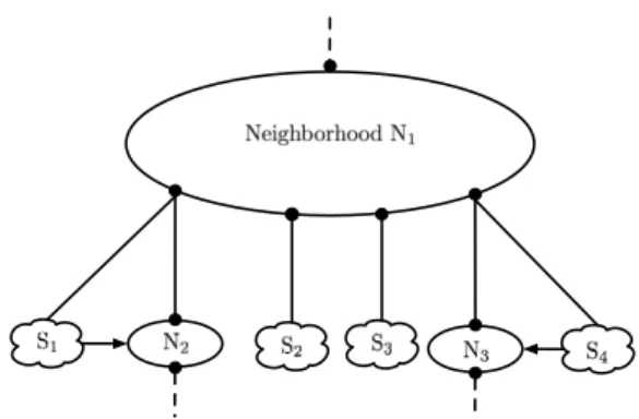
From the perspective of a single vantage point, a subnet can be seen as a set of N responsive interfaces (all being part of a continuous block of M hypothetical interfaces) made of three important components, all of them being depicted in Fig. 1. First, the Ingress router refers to the last router crossed by a packet before reaching the subnet of interest. Second, the Contra-Pivot interface is the IP interface belonging to the subnet that is located on the Ingress router (black circles on Fig. 1). Finally, the Pivot interface refers to any other IP interface in the subnet, all located at the same hop count (gray squares on Fig. 1).

By definition, the Contra-Pivot interface is located at the hop count required to reach a Pivot interface minus one. As such, the Contra-Pivot interface demarcates the subnet under exploration. Finally, in order to ease the subnets location, we introduce the notion of Neighborhood as a location bordered by a set of subnets located at, at most, one hop from each other. From a physical point of view, subnets bordering a same neighborhood should be connected through one router or a mesh of Layer-2/Layer-3 devices.

C. Network Pre-scanning

The very first step of TreeNET consists in listing all IP addresses of the targeted domain, either provided as single addresses, either as IPv4 prefixes. After a shuffling step, which prevents TreeNET from probing consecutive addresses during the next steps (to mitigate network delays), each listed address is probed to check its liveness. Multi-threading is used to make this step as fast as possible.

Due to networking issues, some addresses might not reply during this first probing phase. This is why TreeNET con-ducts a second pre-scanning phase during which the timeout delay used in the first phase is doubled to get as many re-sponsive addresses as possible. An optional third pre-scanning phase can also be conducted.

When a probed address replies within the expected delay, it is saved in a structure we will refer to as the IP dictionary. It stores all responsive IP interfaces and related data, such as the timeout delay which was used when it first replied. All next

probes targeting this interface will use this timeout delay to guarantee new responses.

As unresponsive IP interfaces do not appear in the dictio-nary, they will not be probed again during the next TreeNET steps, such as subnet inference, where all potential IP in-terfaces of a subnet under exploration are considered, one at a time. Therefore, by listing only responsive IPs with a preliminary multi-threaded step, TreeNET buys time for subsequent algorithmic steps.

D. Subnet Inference and Refinement

After the end of the pre-scanning phase, TreeNET infers all subnets containing the IP addresses in the IP dictionary by relying on the subnet inference techniques implemented in ExploreNET. The algorithm starts by probing a given target address (with ICMP ECHO requests, naked or wrapped in UDP or TCP) and estimating its distance from the vantage point as a TTL value. Then, it builds a small subnet (/31 or /30) which encompasses it, sending additional probes on close IP addresses (e.g., which differs by one bit in the two last bits) with the same TTL as the one required to reach the initial target. This first step also considers adjustments of the TTL value used while probing IP addresses other than the target in case the initial target address was a Contra-Pivot interface.

The next step consists in growing the initial subnet by iteratively decrementing its prefix length while checking that the new addresses are indeed part of it. This verification step involves additional probing during which the TTL of the probe packets varies to confirm the position of the targeted IP addresses. ExploreNET eventually stops growing a subnet in two distinct scenarios. In the first scenario, ExploreNET discovers that a new address is not part of the subnet (e.g., second Contra-Pivot interface, interface located at the Pivot TTL plus one, etc.). In such a case, it increments the subnet prefix length by one and returns it together with the list of its responsive interfaces. The second scenario happens when, at a given iteration, the total amount of responsive interfaces within the new subnet is below a threshold value that depends on the current prefix length. Then, ExploreNET stops iterating and returns the subnet with its prefix length incremented by one and the list of its responsive interfaces. Upon receiving the final subnet as inferred by ExploreNET, TreeNET also merges the result with previously inferred subnet(s) which cover(s) the same address ranges to ensure the uniqueness of each subnet at the end of the inference.

It is important to understand that, when a large subnet lacks of responsive interfaces, ExploreNET tends to frag-ment it into several smaller subnets containing groups of responsive interfaces with only one of them containing a valid Contra-Pivot interface, meaning that only this subnet can be considered as sound. To overcome this issue, TreeNET introduces a refinement phase which aims at ensuring any inferred subnet features a valid Contra-Pivot interface. The idea of the refinement phase is the following: TreeNET takes subnets that miss a Contra-Pivot and adjusts their sizes in order to find it. This consists in iteratively decrementing the prefix

Fig. 2. Topology from Fig. 1 seen as a tree – horizontal arrows highlights the subnets acting as links between two routers.

length of the incomplete subnet and probing the new addresses with the TTL that matches the hypothetical hop count of the Contra-Pivot interface. This refinement by expansion stops as soon as one or several Contra-Pivot candidates are found, or when the subnet starts overlapping other measured sound subnets whose TTL to reach Pivot interfaces is different from the one to reach a Pivot in the subnet being expanded. It also stops when the subnet becomes larger than a /20, as no /19 were observed with neither ExploreNET neither TreeNET. The fact that a subnet can have several Contra-Pivot candidates can be due to networking issues (e.g., redirections) or network policies, such as routers having a back-up interface for a subnet in case the first one failed. The absence of visible Contra-Pivot interface is most probably due to networking issues. In a sense, TreeNETapplies a best effort policy while refining subnets. The fact that a subnet can feature a single, several, or no Contra-Pivot motivates the introduction of a classification which can be used to assess the accuracy and soundness of the measurements. It is worth noticing here that IP addresses can respond with TTL that does not match the expected Pivot TTL or Contra-Pivot TTL. We will refer to such addresses as

outliers and our classification takes into account such cases. Each subnet is therefore labeled as Accurate (i.e., it features a single Contra-Pivot interface and no outlier), Odd (i.e., it features two or more Contra-Pivot interfaces and/or some outliers), or Shadow (i.e., no valid Contra-Pivot interface could be found, with or without outliers).

Furthermore, when a subnet is classified as Accurate, each missing IP address that was responsive during pre-scanning is added to this subnet in order to have a list of live interfaces as complete as possible for each subnet. Finally, Shadow subnets are expanded until they collide with sound (i.e., Accurate or

Odd) subnets at the very end of the subnet inference. The purpose of this last refinement is to obtain an upper bound on their size.

E. Tree Construction

Once the targeted domain has been completely analyzed, TreeNET performs Paris traceroute measurements to-wards each inferred subnet, using a Pivot interface as des-tination.

Having routes to every subnet provides knowledge on how they are located with respect to each other. Taking benefit of such an additional information, TreeNET builds a tree rooted at the vantage point and whose leaves are the measured subnets. Each internal node of depth N is labeled with an interface that appears at the Nth _{position in one or several}

traces. The immediate result of this construction is that internal nodes actually represent Neighborhoods. Moreover, the labels of internal nodes can be used to identify the subnets that act as a link between two routers: one has simply to check that a label belongs to a subnet occurring at the same depth. To illustrate this construction, Fig. 2 shows the same topology as shown in Fig. 1 but as a tree, with the horizontal arrows highlighting the subnets acting as links between two routers.

In order to be faithful to the measured topology, the tree should reduce the impact of routing issues caused by traffic engineering (e.g., load balancing [17]). For example, several subnets sharing the same Ingress router should have routes of the same length with the same last replying interfaces, but differences can still occur on the rest of the routes. As a consequence, the tree could feature several branches for these subnets and partial representation of their Neighborhood, rather than having a single branch at the end of which one can obtain a complete representation of the Neighborhood bordering those subnets. To avoid this situation, TreeNET allows internal nodes to have more than one label in such a way that the Neighborhood information in deeper nodes is not lost. As a result, internal nodes with multiple labels constitute no longer a single Neighborhood but rather a superposition of several Neighborhoods. For the sake of simplicity, we will refer to these nodes as multi-label nodes. Post-processing of the fully built tree can however isolate Neighborhoods of a multi-label node from each other.

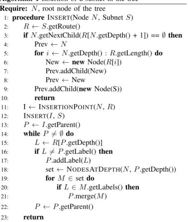
The process of the tree construction is fully described in Algorithm 1. Starting with an empty tree, the algorithm inserts sequentially new subnets in two steps. The first one consists in finding the insertion point defined as the deepest internal node that shares a common label (line 11). In TreeNET, this step is efficiently implemented using additional data structures to avoid visiting the whole tree. Once the insertion point has been found, all missing internal nodes (if any) and the leaf corresponding to the subnet are inserted (lines 3 – 10). The second step consists in moving from the insertion point to the root of the tree while inserting new labels whenever the route differs from current information stored in the tree (lines 12 – 23). In particular, for each node, if the label from the route of the new subnet already appears in another internal node of the tree at the same depth, it is merged with the current node (lines 19 – 21). The final result is a tree in which every label should appear only once.

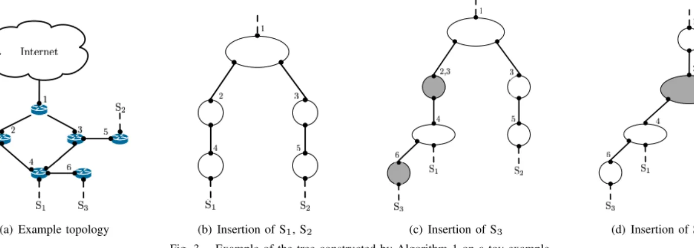
Fig. 3 illustrates the tree construction on a toy exam-ple. Given the topology shown in Fig. 3(a), possible Paris traceroute to subnets S1, S2, and S3 could be{1, 2, 4},

{1, 3, 5}, and {1, 3, 4, 6} respectively. The insertion of S1and

S2is then rather simple, as Fig. 3(b) shows. Fig. 3(c) and 3(d)

illustrates how the insertion of S3 occurs. The insertion point

Algorithm 1 Insertion of a subnet in the tree Require: N , root node of the tree

1: procedure INSERT(Node N , Subnet S)

2: R_{← S.getRoute()}

3: if N .getNextChild(R[N .getDepth() + 1]) ==∅ then

4: Prev← N

5: for i ← N .getDepth() : R.getLength() do

6: New← new Node(R[i])

7: Prev.addChild(New) 8: Prev← New 9: Prev.addChild(new Node(S)) 10: return 11: I← INSERTIONPOINT(N , R) 12: INSERT(I, S) 13: P ← I.getParent() 14: while P 6= ∅ do 15: L ← R[P .getDepth()] 16: if L6= P .getLabel() then 17: P .addLabel(L)

18: set← NODESATDEPTH(N , P .getDepth())

19: for M ∈ set do

20: if L∈ M .getLabels() then

21: P .merge(M )

22: P _{← P .getParent()}

23: return

is obviously the node having the label 4. As the parent node does not have the label 3, such a label is added; however, label 3 already appears in the tree, therefore the branch is merged with the node containing both labels 2 and 3. In the final tree, all non-null (i.e., not 0.0.0.0) labels appear only once.

As implied in the previous paragraph, the routes obtained with Paris traceroute are not always complete, i.e., they feature 0.0.0.0 interface(s) along the way. As TreeNET does not consider these labels while looking for the insertion point, this leads to one branch per distinct interface following a 0.0.0.0 interface. While this does not affect deeper internal nodes, this can lead to splitting a large internal node into several ones. Specially when the interface is labeled as 0.0.0.0 due to a delay or a black-listing of the vantage point by that interface, preventing it from replying to any subsequent probe. This typically occurs with the first hops to a remote network (which are often common to all routes): some routes will feature the proper interface(s) while others will not.

To mitigate this issue, TreeNET always starts building the tree using only subnets that feature a complete route (i.e., with no occurrence of 0.0.0.0). Then, before inserting any subnet with an incomplete route, TreeNET finds the most similar route already stored in the tree and replaces 0.0.0.0 interface(s) of the incomplete route with the interface(s) at the same index(es) in the selected route.

F. Router Inference

A fully built tree provides a good knowledge of the topology, as it gives an idea of how many interfaces border

(a) Example topology (b) Insertion of S1, S2 (c) Insertion of S3 (d) Insertion of S3(2)

Fig. 3. Example of the tree constructed by Algorithm 1 on a toy example.

an internal node, which is either a Neighborhood, either a superposition of Neighborhoods. Given #L the amount of labels of a node, #S the amount of children subnets, #I the total amount of labels from child internal nodes, and #C the amount of crossed subnets (i.e., subnets which contain the label of a child internal node), the amount N of interfaces an internal node is given by

N _{= #L + #I + #S − #C. (1)} The amount of labels#L can be assimilated to the number of interfaces through which packets enter the Neighborhood(s), while #I + #S − #C refers to the number of outgoing interfaces.

Not only the tree provides an idea of the number of interfaces of each internal node, but it also gives some of these interfaces. The labels themselves are interfaces, but moreover, subnets classified as Accurate during subnet inference feature a valid Contra-Pivot interface which, by definition, is the interface of a router. Odd subnets also feature at least one valid Contra-Pivot. Therefore, for each internal node, one can list all labels and each Contra-Pivot of each child Accurate or

Odd subnet. Then, one can use an alias resolution technique on them to infer one or several routers. After that, internal nodes do not need to be abstracted as Neighborhoods (or superimpositions) any longer, and one can build a full router – subnet topology of the measured network. The alias resolution also helps to disambiguate multi-label nodes, as interfaces of routers belonging to distinct (superposed) Neighborhoods should never be associated together.

In TreeNET, the router inference consists in a combination of three different alias resolution techniques: Ally [18], IP-ID counter velocity check (which is reminiscent of Radar-Gun [19]), and reverse DNS association.

For every interface of an internal node/Neighborhood, TreeNETcollects i IP-IDs (i is at least three) and evaluates the wall clock time (in microseconds) between the acquisition of each ID, leading to i - 1 delays. While the wall clock time might not be necessarily faithful to the delay between the generation of two IP-IDs on a remote device, it is a

Fig. 4. Schematic view of the data used for the velocity range technique.

reasonable and exploitable estimation. In addition to the IP-IDs and delays, the reverse DNS for each IP address is also retrieved when available.

Once all the aforementioned data has been collected for every interface, the association process starts. When IP-IDs and associated delays are available, TreeNET first considers association by Ally. The idea of Ally is very simple: one probes a first interface, retrieves an IP-ID x, then obtains another IP-ID y from a second interface, and a third ID z from the first one. If the inequality x < y < z with z - x being reasonably small is verified, one can assume both probed interfaces actually belong to the same router. Therefore, in the context of TreeNET, one just has to find a triplet of IP-IDs from two distinct interfaces which form a succession to use Ally. To locate IP-IDs chronologically, each collected ID has an associated token, an integer unique to each probe that is given by a counter incremented each time a token is drawn.

However, the IP-ID counters can evolve quite fast, therefore mitigating the efficiency of Ally in many cases. To overcome this issue, the second technique implemented in TreeNET rather estimates the velocity of each counter for each interface (the three IP-ID mentioned above) and associates interfaces together when their velocity is similar, which is the same idea as RadarGun [19]. This is why delays between getting each IP-ID are being collected.

However, the velocity of a counter is not constant and fluctuates, and to model this, TreeNET does not compute a single velocity per interface but rather a range of velocities, with a velocity being computed for every pair of consecutive IP-IDs. Moreover, as IP-ID counters are encoded on 16 bits, they can rollover on a regular basis, and it is not unlikely to have two or more rollovers for interfaces belonging to routers dealing with large traffic. For every pair of consecutive IP-IDs (denoted as i and i+ 1 and the delay between those IP-IDs is

denoted di), we consider a variable xito model the amount of

rollovers. In Fig. 4, we illustrate the data involved in our alias resolution technique based on IP-ID counter velocity and the variables for each pair of consecutive IP-IDs.

To be able to compute coherent velocities, one must find a value for every xisuch that the velocities are reasonably close

to each other. Our approach consists in assigning a value from 0 to a maximum (e.g., 50) to x0and, for each value, resolving

i_{− 2 equations to find every x}i with i being greater than 0.

The equation is the following i_{1− i0+ 65535 × x0}

d₀ =

i_{i+1− i}i+ 65535 × xi

di

. ₍₂₎ As it is possible to have the inequality ii+1 < ii due to a

rollover between the first IP-ID of the pair and the second one, we replace−iiby+(65535−ii) when this occurs to accurately

express the amount of times the counter was incremented. Since it is extremely rare to find an integer, non-zero solution for every xi, we rather solve such equations in the real

domain and round the results afterwards. If all solutions are positive and if the rounding error (i.e., the difference between the rounded result and the real value) is below a threshold (e.g., 0.35), the rounded solutions are kept, otherwise the next value for x0is being considered until the maximum. If the maximum

value is reached without finding a solution, we consider the counter to have an infinite velocity, represented by the range [0, 65535].

If an integer value is found for every xi, the velocities are

obtained with the following formula: vi=

ii+1− ii+ 65535 × xi

di

. ₍₃₎

Of course, if ii is greater than ii+1, the term −ii is again

replaced with +(65535 − ii).

The final step consists in retrieving the maximum and minimum velocity obtained for the IP addresses. Afterwards, interfaces are associated if their respective ranges of velocity overlap. As we observed several ranges being very close to each other without overlapping, we added a tolerance value (e.g., 0.3) which slightly extends the largest range such that it overlaps close ranges. Finally, it is worth noting we always associate together interfaces for which the velocity is computed as infinite (i.e., [0, 65535]).

If neither Ally nor the velocity range technique can be used, reverse DNS association is considered. It is worth noting that if IP-IDs are available and if the two previous techniques rejected the association, reverse DNS is not considered. In other words, reverse DNS is the last resort technique. The technique itself is very simple: splitting the DNS of two IP interfaces at dots, they will be associated if and only if they have the same amount of components and if only the first ones differ between both IP addresses. We did not elaborate our reverse DNS technique further because of the need for additional inputs, such as the naming conventions found in a particular network.

0.0 0.1 0.2 0.3 0.4 0.5 0.6 0.7 0.8 0.9 1.0

Accuracy

Cumulative Density Function

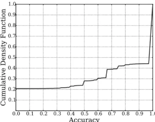
Fig. 5. Preliminary performance results for our alias resolution scheme.

III. EVALUATION

In this section, we evaluate the performance of TreeNET. We first provide preliminary results for our three alias res-olution scheme (Sec. III-A) and, next, we compare subnet inference of TreeNET with ExploreNET (Sec. III-B) on a ground truth and several ASes. We also mention some preliminary results which could guide future study of the mea-sured ASes (Sec. III-C). Subnets and aliases collected during our measurement campaign are freely available: https:// github.com/JefGrailet/treenet/tree/master/ v2/Measurements

A. Alias Resolution

To assess our alias resolution scheme described in Sec. II-F, we relied on a dataset provided by iPlane [16]. It is made of a list of 57,806 routers with their aliases as observed in iPlane traceroute. Aliases are determined by using standard IP-ID technique and identical return TTLs when probed at the same time. It should be noted that this dataset is updated every two months and that our GitHub repository provides the dataset which was available at the time of our measurements. For each alias (given as a list of interfaces), we run our resolution technique and define an accuracy rate, i.e., the size (i.e., amount of interfaces) of the largest alias inferred by TreeNET for this list divided by the number of responding interfaces from that list. As a consequence, a value of 1 means that we obtain the same results as iPlane with respect to responsive interfaces. On the contrary, a value of 0 means that we are not able to identify the listed interfaces as aliases at all. Measurements were done on November 19th_{, 2015, collecting}

four IP-IDs for each responsive interface.

On the set of 57,806 routers, 26% of them were not responding to our probes. No accuracy rate has been computed on those routers. The accuracy rate for the remaining 74% of the routers is given, as a cumulative distribution function, on Fig. 5. The most important result here is that, in 55% of the cases, our alias resolution provides the same results as the iPlane dataset. The second main result is that, for a bit more than 70% of the dataset, we have an accuracy rate of at least 50%. Those results are promising and we leave as a future work a better characterization of our alias resolution technique and potential improvements of it. In particular, we

plan to elaborate on the amount of collected IP-IDs and the effects of other parameters of our velocity-based technique we previously mentioned.

B. Subnet Inference

In order to evaluate the subnet inference proposed by TreeNET with respect to ExploreNET, we implemented a slightly edited version of ExploreNET using the same input/output schemes as TreeNET and targeted different ASes as well as a ground truth network (an academic network for which we have access to the actual topology – access to that network topology is, obviously, not allowed outside the campus) with both of them.

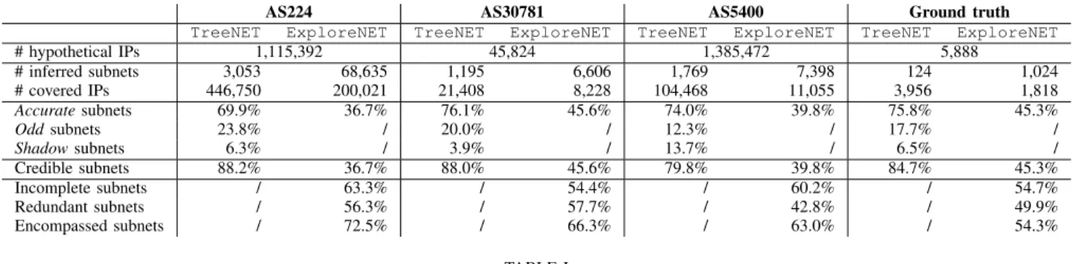
We decided to conduct measurements on three ASes: AS224, AS5400 and AS30781. The first two are comparable regarding the amount of hypothetical IP addresses (a bit more than one million in both cases) but have a different role in the Internet topology: AS224 is a stub AS (i.e., all traffic coming in and out of it goes through a single path) while AS5400 is a transit AS (i.e., it acts as a link between other ASes). AS30781, on the other hand, is another transit AS but of a much smaller scale (with a maximum of 45,824 hypothetical IP addresses), which is interesting for a comparison with AS5400. The datasets we obtained from them are available on https:// github.com/JefGrailet/treenet/tree/master/ v2/Measurements. Additionnal datasets for other ASes will be progressively added on the same page.

In the case of the ground truth, we were able to check the re-sults with a network administrator, and discovered that 86.3% of our measured subnets were correct in terms of prefix with respect to the actual topology, the problematic results being caused by very specific cases. These difficult cases notably included loop-back interfaces from distinct subnets (sometimes /32 subnets) whose TTL were similar and for which the IPv4 addresses were consecutives, and were therefore considered to be on the same subnet. The inferred routers were also confirmed by the actual network, therefore demonstrating the relevancy of the tree structure and proving again the accuracy of our alias resolution scheme.

To assess the soundness of subnets measured by TreeNET, we introduce the notion of credibility of a subnet. A subnet is considered as credible if less than 10% of its listed interfaces are Contra-Pivot candidates and more than 70% of them are Pivot interfaces, as we consider a subnet cannot be sound if more than 20% of its interfaces are outliers. These numbers are however arbitrary and could be adapted for specific networks where the amount of outliers is assumed to be high. The purpose of this metric is to evaluate if an Odd subnet is a good measurement, an Accurate subnet being de facto credible while Shadow subnets are never considered as credible.

Finally, we also use two additional metrics on datasets ob-tained through ExploreNET: redundancy and encompassed ratios. The redundancy ratio denotes how many subnets in the datasets are equivalent with previously listed subnets, since ExploreNETdoes not merge similar subnets like TreeNET does. The encompassed ratio, on the other hand, quantifies how

many subnets inferred by ExploreNET are strictly smaller than overlapping subnets obtained by TreeNET, in order to check if the latter handles large subnets better than the former. Our results are presented in Table I. One can immediately notice a striking improvement due to TreeNET. It is indeed remarkable how TreeNET is able to infer a smaller amount of subnets than ExploreNET while covering much more ad-dresses and having a high proportion of Accurate subnets. The ratios of incomplete, redundant, and encompassed subnets for each network further demonstrate that the refinements operated by TreeNET over the results of ExploreNET drastically improves the inferred subnets regarding both credibility (in the broad sense) and coverage of the measured networks.

Furthermore, the introduction of Odd subnets in TreeNET overcomes a limitation of ExploreNET: indeed, the latter assumes that a subnet necessarily owns a single Contra-Pivot interface. Therefore, ExploreNET can stop the inference when it discovers two potential Contra-Pivot interfaces at once. Unfortunately, this prevents it from properly inferring a large subnet when there is, for example, a back-up Contra-Pivot interface. It also tends to ignore outliers (e.g., an IP interface located at the Pivot TTL + 1, which can occur due to specific network policies), that could appear in measurements conducted by TreeNET due to subnet merging. Thus, not only the refinements help to find sounder subnets, but they also relax the definition of a subnet to some extent and allows the discovery of more exotic network configurations.

C. Preliminary results

Even if the focus of this paper is the description and evaluation of TreeNET, we can already provide directions for future analysis of the networks measured with it. In particular, the datasets we collected can be analyzed to compute the distribution of the subnet prefix lengths in each AS and our ground truth. A first look at Fig. 6 already highlights an interesting property: the proportion for each prefix length varies from one network to another, and while /31 and /30 subnets are inevitably the most common ones (as already observed with ExploreNET [8]), other prefix lengths are not used in the same manner by each network.

For example, /24 subnets are particularly common in our dataset from AS224, which is a stub AS. An interesting perspective for future research would be to compare the results obtained by TreeNET on several stub ASes to determine if the proportion of /24 subnets is a common feature of stub ASes or an AS224 specificity.

However, an in-depth analysis of the data would require more metrics and modeling formalisms suited for router – subnet topologies, which are left for future work.

IV. CONCLUSION

In this paper, we introduced TreeNET, a new tool collect-ing and manipulatcollect-ing subnet topology information to discover the router – subnet topology of a target network. Using as a basis ExploreNET, a state of the art subnet inference tool, TreeNET adds subnet refinement mechanisms along with a

AS224 AS30781 AS5400 Ground truth TreeNET ExploreNET TreeNET ExploreNET TreeNET ExploreNET TreeNET ExploreNET

# hypothetical IPs 1,115,392 45,824 1,385,472 5,888 # inferred subnets 3,053 68,635 1,195 6,606 1,769 7,398 124 1,024 # covered IPs 446,750 200,021 21,408 8,228 104,468 11,055 3,956 1,818 Accuratesubnets 69.9% 36.7% 76.1% 45.6% 74.0% 39.8% 75.8% 45.3% Oddsubnets 23.8% / 20.0% / 12.3% / 17.7% / Shadowsubnets 6.3% / 3.9% / 13.7% / 6.5% / Credible subnets 88.2% 36.7% 88.0% 45.6% 79.8% 39.8% 84.7% 45.3% Incomplete subnets / 63.3% / 54.4% / 60.2% / 54.7% Redundant subnets / 56.3% / 57.7% / 42.8% / 49.9% Encompassed subnets / 72.5% / 66.3% / 63.0% / 54.3% TABLE I

Comparison between TreeNET and ExploreNET for several ASes and our ground truth.

/20 /21 /22 /23 /24 /25 /26 /27 /28 /29 /30 /31 Prefix length 0 10 20 30 40 50 60 70 Subnet distribution (%) AS224 AS5400 AS30781 Ground truth

Fig. 6. Distribution of the subnet prefix length in the observed networks.

tree-like structure which not only gives an overview of the network but also eases router discovery via alias resolution techniques.

We were able to demonstrate the benefits of TreeNET regarding subnet inference through a comparative study with ExploreNET on a ground truth network and several ASes. We also obtained promising results for the alias resolution scheme currently implemented in TreeNET, both on our private ground truth and a publicly available dataset provided by iPlane. The datasets we obtained from the mentioned ASes and the aliases list provided by iPlane we used are pub-licly available on https://github.com/JefGrailet/ treenetalong with the sources of TreeNET.

Future works involve in-depth evaluation of TreeNET (in particular the efficiency of the pre-scanning phase and the alias resolution scheme compared to RadarGun), large-scale mea-surement campaigns and in-depth study of our datasets through modeling formalisms suited for router – subnet topologies. We are also planning to use TreeNET to elaborate Layer-2 devices inference techniques in the long term.

ACKNOWLEDGMENTS

This work is partially funded by the European Commission funded mPlane ICT-318627 project.

REFERENCES

[1] R. Pastor-Satorras and A. Vespignani, Evolution and Structure of the

Internet: A Statistical Physics Approach. Cambridge University Press,

2004.

[2] B. Donnet and T. Friedman, “Internet topology discovery: a survey,”

IEEE Communications Surveys and Tutorials, vol. 9, no. 4, December

2007.

[3] Y. Shavitt and N. Zilberman, “Geographical Internet PoP level maps,” in Proc. Traffic Monitoring and Analysis Workshop (TMA), March 2012. [4] D. Feldman, Y. Shavitt, and N. Zilberman, “A structural approach for PoP geo-location,” Computer Networks (COMNET), vol. 56, no. 3, pp. 1029–1040, February 2012.

[5] M. E. Tozal and K. Sarac, “TraceNET: an Internet topology data collector,” in Proc. ACM/USENIX Internet Measurement Conference

(IMC), November 2010.

[6] M. E. Tozal and K. Sarac, “Estimating network layer subnet character-istics via statistical sampling,” in Proc. IFIP Networking, May 2012. [7] M. Gunes and K. Sarac, “Inferring subnets in router-level topology

collection studies,” in Proc. ACM/USENIX Internet Measurement

Con-ference (IMC), November 2007.

[8] M. E. Tozal and K. Sarac, “Subnet level network topology mapping,” in

Proc. IEEE International Performance Computing and Communications

Conference (IPCCC), November 2011.

[9] J. Mogul and J. Postel, “Internet standard subnetting procedure,” Internet Engineering Task Force, RFC 950, August 1985.

[10] K. Keys, “Internet-scale IP alias resolution techniques,” ACM

SIG-COMM Computer Communication Review, vol. 40, no. 1, pp. 50–55,

January 2010.

[11] P. Marchetta, P. M´erindol, B. Donnet, A. Pescap´e, and J.-J. Pansiot, “Topology discovery at the router level: a new hybrid tool targeting ISP networks,” IEEE Journal on Selected Areas in Communication, Special

Issue on Measurement of Internet Topologies, vol. 29, no. 6, pp. 1776–

1787, October 2011.

[12] P. M´erindol, B. Donnet, O. Bonaventure, and J.-J. Pansiot, “On the impact of layer-2 on node degree distribution,” in Proc. ACM/USENIX

Internet Measurement Conference (IMC), November 2010.

[13] P. Marchetta, P. M´erindol, B. Donnet, A. Pescap´e, and J.-J. Pansiot, “Quantifying and mitigating IGMP filtering in topology discovery,” in Proc. IEEE Global Communications Conference (GLOBECOM), December 2012.

[14] V. Jacobson et al., “traceroute,” UNIX,” man page, 1989, see source code: ftp://ftp.ee.lbl.gov/traceroute.tar.gz.

[15] B. Augustin, X. Cuvellier, B. Orgogozo, F. Viger, T. Friedman, M. Lat-apy, C. Magnien, and R. Teixeira, “Avoiding traceroute anomalies with Paris traceroute,” in Proc. ACM/USENIX Internet Measurement

Conference (IMC), October 2006.

[16] H. V. Madhyastha, T. Isdal, M. Piatek, C. Dixon, T. Anderson, A. Kr-ishnamurthy, and A. Venkataramani, “iPlane: An information plane for distributed services,” in Proc. USENIX Symposium on Operating

Systems Design and Implementation (OSDI), November 2006, see http:

//iplane.cs.washington.edu/data/alias lists.txt.

[17] B. Augustin, R. Teixeira, and T. Friedman, “Measuring load-balanced paths in the Internet,” in Proc. ACM/USENIX Internet Measurement

Conference (IMC), November 2007.

[18] N. Spring, R. Mahajan, and D. Wetherall, “Measuring ISP topologies with Rocketfuel,” in Proc. ACM SIGCOMM, August 2002.

[19] A. Bender, R. Sherwood, and N. Spring, “Fixing Ally’s growing pains with velocity modeling,” in Proc. ACM/USENIX Internet Measurement